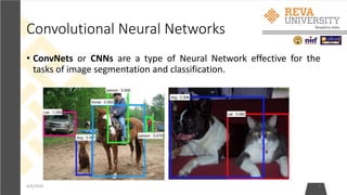
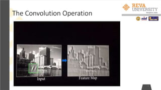
This document provides an outline and overview of training convolutional neural networks. It discusses update rules like stochastic gradient descent, momentum, and Adam. It also covers techniques like data augmentation, transfer learning, and monitoring the training process. The goal of training a CNN is to optimize its weights and parameters to correctly classify images from the training set by minimizing output error through backpropagation and updating weights.

1. 18/1/2020
Training Convolutional Neural Networks –II
Nimrita Koul

2. Outline
• A Quick Recap
• Training CNN –II
• Update Rules
• Data Augmentation
• Transfer Learning
• Hands on with Python
8/1/2020 2

3. Convolutional Neural Networks
• ConvNets or CNNs are a type of Neural Network effective for the
tasks of image segmentation and classification.
4/6/2020 3

4. 4/6/2020 4

5. The Convolution Operation
4/6/2020 5

6. Rectified Linear Unit(ReLU) & Pooling
4/6/2020 6
ReLU: Output=Max(zero, input)
Max Pooling

7. 4/6/2020 7

8. A Neuron Learns by adjusting its weights
4/6/2020 8

9. What is “Training” for a CNN?
4/6/2020 9

10. Mini Batch Stochastic Gradient Algorithm
• The Mini batch stochastic gradient descent algorithm steps:
• Loop:
• Sample a batch of data.
• Forward prop it through the graph (network) and get loss.
• Backprop to calculate the gradients.
• Update the parameters using the gradients.
4/6/2020 10

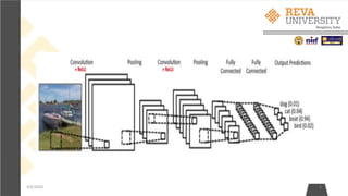
11. The CNN Training Process
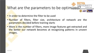
• Parameters - Number of filters, filter sizes, architecture of the network etc.
are fixed before Step 1 and do not change during training process – only
the values of the filter matrix and connection weights get updated.
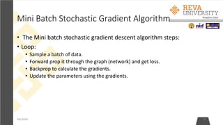
• Step1: Initialize all filters and parameters / weights with random values.
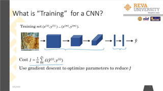
• Step2: The network takes a training image as input, goes through the
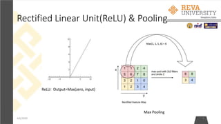
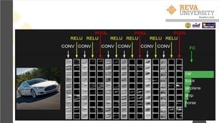
forward propagation step (convolution, ReLU and pooling operations, the
Fully Connected layer) and finds the output probabilities for each class.
• Lets say the output probabilities for the boat image above are [0.3, 0.3, 0.1, 0.2,0.1]
• Since weights are randomly assigned for the first training example, output
probabilities are also random.
4/6/2020 11

12. • Step3: Calculate the total error at the output layer (summation
over all 4 classes)
• Total Error = ∑ ½ (target probability – output probability) ²
• Step4: Use Backpropagation to calculate the gradients of the
error with respect to all weights in the network and
use gradient descent to update all filter values / weights and
parameter values to minimize the output error.
4/6/2020 12

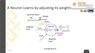
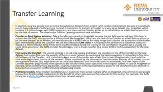
13. • The weights are adjusted in proportion to their contribution to the total error.
• When the same image is input again, output probabilities might now be [0.6,
0.1, 0.1, 0.1,0.1], which is closer to the target vector [1, 0, 0,0, 0].
• This means that the network has learnt to classify this particular image
correctly by adjusting its weights / filters such that the output error is
reduced.
4/6/2020 13

14. • Step5: Repeat steps 2-4 with all images in the training set.
• The above steps train the ConvNet – this essentially means that all
the weights and parameters of the ConvNet have now been optimized
to correctly classify images from the training set.
4/6/2020 14

15. Data Preprocessing
4/6/2020 15
• Data Normalization - To get the Zero centered data, we calculate
mean of input data and then apply standard deviation.
X -= np.mean(X, axis = 1)
X /= np.std(X, axis = 1)
•Image Normalization - Subtract the mean image (with same shape
as that of input image) from the input image. No Standard
deviation.

16. Weight Initialization
• What happens when we initialize all Weights to zero?
• All the neurons will do exactly the same thing. They will have the
same gradient and they will have the same update.
• First idea is to initialize the w's with small random numbers:
• The standard deviations is going to zero in deeper networks and the
gradient will vanish sooner.
• If we initialize the weights to big numbers, the network will explode.
4/6/2020 16

17. Transfer Learning
• If you are using a specific NN architecture that has been trained before, you can use this pre-trained parameters/weights instead of
• random initialization to solve your problem. It can help you boost the performance of the NN.
• The pre-trained models might have trained on a large datasets like ImageNet, Ms COCO, or pascal and took a lot of time to learn those parameters/weights with optimized hyper-
parameters. This can save you a lot of time.
• Lets see an example:
• Lets say you have a cat classification problem which contains 3 classes Tigger, Misty and neither.
• You don't have much a lot of data to train a NN on these images.
• Andrew recommends to go online and download a good NN with its weights, remove the softmax activation layer and put your own one and make the network learn only the new layer
while other layer weights are fixed/frozen.
• Frameworks have options to make the parameters frozen in some layers using trainable = 0 or freeze = 0
• One of the tricks that can speed up your training, is to run the pre-trained NN without final softmax layer and get an intermediate representation of your images and save them to disk.
And then use these representation to a shallow NN network. This can save you the time needed to run an image through all the layers.
• Its like converting your images into vectors.
• Another example:
• What if in the last example you have a lot of pictures for your cats.
• One thing you can do is to freeze few layers from the beginning of the pre-trained network and learn the other weights in the network.
• Some other idea is to throw away the layers that aren't frozen and put your own layers there.
• Another example:
• If you have enough data, you can fine tune all the layers in your pre-trained network but don't random initialize the parameters, leave the learned parameters as it is and learn from there.
4/6/2020 17

18. Data Augmentation
• If data is increased, your deep NN will perform better. Data augmentation is one of the techniques that deep learning uses to increase the
performance of deep NN. The majority of computer vision applications needs more data right now. Some data augmentation methods that are used
for computer vision tasks includes:
• Mirroring.
• Random cropping.
• The issue with this technique is that you might take a wrong crop.
• The solution is to make your crops big enough.
• Rotation.
• Shearing.
• Local warping.
• Color shifting.
• For example, we add to R, G, and B some distortions that will make the image identified as the same for the human but is different for the computer.
• In practice the added value are pulled from some probability distribution and these shifts are some small. Makes your algorithm more robust in
changing colors in images. There are an algorithm which is called PCA color augmentation that decides the shifts needed automatically. Implementing
distortions during training:
• You can use a different CPU thread to make you a distorted mini batches while you are training your NN.
• Data Augmentation has also some hyperparameters. A good place to start is to find an open source data augmentation implementation and then use
it or fine tune these hyperparameters.
4/6/2020 18

19. 4/6/2020 19
•Baby sitting the learning process
1.Preprocessing of data.
2.Choose the architecture.
3.Make a forward pass and check the loss (Disable regularization). Check if the loss is reasonable.
4.Add regularization, the loss should go up!
5.Disable the regularization again and take a small number of data and try to train the loss and reach zero loss.
•You should overfit perfectly for small datasets.
6.Take your full training data, and small regularization then try some value of learning rate.
•If loss is barely changing, then the learning rate is small.
•If you got NAN then your NN exploded and your learning rate is high.
•Get your learning rate range by trying the min value (That can change) and the max value that doesn't explode the network.
7.Do Hyperparameters optimization to get the best hyperparameters values.
•

20. • Hyperparameter Optimization
• Try Cross validation strategy.
• Run with a few ephocs, and try to optimize the ranges.
• Its best to optimize in log space.
• Adjust your ranges and try again.
• Its better to try random search instead of grid searches (In log space)
4/6/2020 20

21. Training II
• Optimization algorithms:
• Problems with stochastic gradient descent:
• if loss quickly in one direction and slowly in another (For only two variables), you will
get very slow progress along shallow dimension, jitter along steep direction. Our NN
will have a lot of parameters then the problem will be more.
• Local minimum or saddle points
• If SGD went into local minimum we will stuck at this point because the gradient is zero.
• Also in saddle points the gradient will be zero so we will stuck.
• Saddle points says that at some point:
• Some gradients will get the loss up.
• Some gradients will get the loss down.
• And that happens more in high dimensional (100 million dimension for example)
• The problem of deep NN is more about saddle points than about local minimum because
deep NN has high dimensions (Parameters)
• Mini batches are noisy because the gradient is not taken for the whole batch.
4/6/2020 21

22. 4/6/2020 22
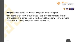
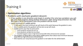
SGD + momentum:
•Build up velocity as a running mean of gradients:
•# Computing weighted average. rho best is in range [0.9 - 0.99] V[t+1] = rho * v[t] + dx x[t+1] = x[t] - learningRate * V[t+1]
•V[0] is zero.
•Solves the saddle point and local minimum problems.
•It overshoots the problem and returns to it back.

23. 4/6/2020 23
•Nestrov momentum:
•dx = compute_gradient(x) old_v = v v = rho * v - learning_rate * dx x+= -rho * old_v + (1+rho) * v
•Doesn't overshoot the problem but slower than SGD + momentum
•AdaGrad
•grad_squared = 0 while(True): dx = compute_gradient(x) # here is a problem, the grad_squared isn't decayed (gets so large) grad_squared += dx * dx x -= (learning_rate*dx) / (np.sqrt(grad_squared) + 1e-7)
•RMSProp
•grad_squared = 0 while(True): dx = compute_gradient(x) #Solved ADAgra grad_squared = decay_rate * grad_squared + (1-grad_squared) * dx * dx x -= (learning_rate*dx) / (np.sqrt(grad_squared) + 1e-7)
•People uses this instead of AdaGrad

24. 4/6/2020 24
•Adam
•Calculates the momentum and RMSProp as the gradients.
•It need a Fixing bias to fix starts of gradients.
•Is the best technique so far runs best on a lot of problems.
•With beta1 = 0.9 and beta2 = 0.999 and learning_rate = 1e-3 or 5e-4 is a great starting point for many models!
•Learning decay
•Ex. decay learning rate by half every few epochs.
•To help the learning rate not to bounce out.
•Learning decay is common with SGD+momentum but not common with Adam.
•Dont use learning decay from the start at choosing your hyperparameters. Try first and check if you need decay or not.
•All the above algorithms we have discussed is a first order optimization.
•

25. • Second order optimization
• Use gradient and Hessian to from quadratic approximation.
• Step to the minima of the approximation.
• What is nice about this update?
• It doesn't has a learning rate in some of the versions.
• But its unpractical for deep learning
• Has O(N^2) elements.
• Inverting takes O(N^3).
• L-BFGS is a version of second order optimization
• Works with batch optimization but not with mini-batches.
• In practice first use ADAM and if it didn't work try L-BFGS.
• Some says all the famous deep architectures uses SGS + Nestrov momentum
•
4/6/2020 25

26. • Regularization
• So far we have talked about reducing the training error, but we care about most is how our model will handle unseen data!
• What if the gab of the error between training data and validation data are too large?
• This error is called high variance.
• Model Ensembles:
• Algorithm:
• Train multiple independent models of the same architecture with different initializations.
• At test time average their results.
• It can get you extra 2% performance.
• It reduces the generalization error.
• You can use some snapshots of your NN at the training ensembles them and take the results.
• Regularization solves the high variance problem. We have talked about L1, L2 Regularization.
• Some Regularization techniques are designed for only NN and can do better.
• Drop out:
• In each forward pass, randomly set some of the neurons to zero. Probability of dropping is a hyperparameter that are 0.5 for almost cases.
• So you will chooses some activation and makes them zero.
• It works because:
• It forces the network to have redundant representation; prevent co-adaption of features!
• If you think about this, It ensemble some of the models in the same model!
• At test time we might multiply each dropout layer by the probability of the dropout.
• Sometimes at test time we don't multiply anything and leave it as it is.
• With drop out it takes more time to train.
•
4/6/2020 26

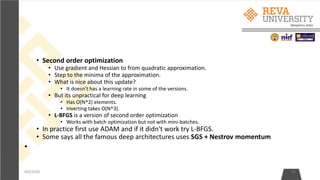
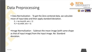
27. • Data augmentation:Another technique that makes Regularization.
• Change the data!
• For example flip the image, or rotate it.
• Example in ResNet:
• Training: Sample random crops and scales:
• Pick random L in range [256,480]
• Resize training image, short side = L
• Sample random 224x244 patch.
• Testing: average a fixed set of crops
• Resize image at 5 scales: {224, 256, 384, 480, 640}
• For each size, use 10 224x224 crops: 4 corners + center + flips
• Apply Color jitter or PCA
• Translation, rotation, stretching.
4/6/2020 27

28. • Drop connect
• Like drop out idea it makes a regularization.
• Instead of dropping the activation, we randomly zeroing the weights.
• Fractional Max Pooling
• Cool regularization idea. Not commonly used.
• Randomize the regions in which we pool.
• Stochastic depth
• New idea.
• Eliminate layers, instead on neurons.
• Has the similar effect of drop out but its a new idea.
4/6/2020 28

29. • Transfer learning:
• Some times your data is overfitted by your model because the data is small
not because of regularization.
• You need a lot of data if you want to train/use CNNs.
• Steps of transfer learning
• Train on a big dataset that has common features with your dataset. Called
pretraining.
• Freeze the layers except the last layer and feed your small dataset to learn only the
last layer.
• Not only the last layer maybe trained again, you can fine tune any number of layers
you want based on the number of data you have
•
Transfer learning is the normal not an exception.
4/6/2020 29

30. 4/6/2020 30

31. • ensorflow (Google)
• Code are two parts:
• Define computational graph.
• Run the graph and reuse it many times.
• Tensorflow uses a static graph architecture.
• Tensorflow variables live in the graph. while the placeholders are feed each
run.
• Global initializer function initializes the variables that lives in the graph.
• Use predefined optimizers and losses.
• You can make a full layers with layers.dense function.
•
4/6/2020 31

32. State of Computer Vision
• For a specific problem we may have a little data for it or a lots of data. Speech recognition problems for example has a big amount
of data, while image recognition has a medium amount of data and the object detection has a small amount of data nowadays.
• If your problem has a large amount of data, researchers are tend to use:
• Simpler algorithms.
• Less hand engineering.
• If you don't have that much data people tend to try more hand engineering for the problem "Hacks". Like choosing a more
complex NN architecture.
• Because we haven't got that much data in a lot of computer vision problems, it relies a lot on hand engineering.
• We will see in the next chapter that because the object detection has less data, a more complex NN architectures will be
presented.
• Tips for doing well on benchmarks/winning competitions:
• Ensembling.
• Train several networks independently and average their outputs. Merging down some classifiers. After you decide the best
architecture for your problem, initialize some of that randomly and train them independently.
• This can give you a push by 2% But this will slow down your production by the number of the ensembles. Also it takes more
memory as it saves all the models in the memory. People use this in competitions but few uses this in a real production. Multi-crop
at test time. Run classifier on multiple versions of test versions and average results.
• There is a technique called 10 crops that uses this. This can give you a better result in the production. Use open source code
• Use architectures of networks published in the literature. Use open source implementations if possible. Use pretrained models
and fine-tune on your dataset.
4/6/2020 32

33. What are the parameters to be optimized?
4/6/2020 33
• In order to determine the filter to be used
• Number of filters, filter size, architecture of network are the
parameters decided before training starts
• More is the number of filters, more image features get extracted and
the better our network becomes at recognizing patterns in unseen
images.

34. Transfer Learning
• In practice, very few people train an entire Convolutional Network from scratch (with random initialization), because it is relatively
rare to have a dataset of sufficient size. Instead, it is common to pretrain a ConvNet on a very large dataset (e.g. ImageNet, which
contains 1.2 million images with 1000 categories), and then use the ConvNet either as an initialization or a fixed feature extractor
for the task of interest. The three major Transfer Learning scenarios look as follows:
• ConvNet as fixed feature extractor. Take a ConvNet pretrained on ImageNet, remove the last fully-connected layer (this layer's
outputs are the 1000 class scores for a different task like ImageNet), then treat the rest of the ConvNet as a fixed feature extractor
for the new dataset. In an AlexNet, this would compute a 4096-D vector for every image that contains the activations of the hidden
layer immediately before the classifier. We call these features CNN codes. It is important for performance that these codes are
ReLUd (i.e. thresholded at zero) if they were also thresholded during the training of the ConvNet on ImageNet (as is usually the
case). Once you extract the 4096-D codes for all images, train a linear classifier (e.g. Linear SVM or Softmax classifier) for the new
dataset.
• Fine-tuning the ConvNet. The second strategy is to not only replace and retrain the classifier on top of the ConvNet on the new
dataset, but to also fine-tune the weights of the pretrained network by continuing the backpropagation. It is possible to fine-tune
all the layers of the ConvNet, or it's possible to keep some of the earlier layers fixed (due to overfitting concerns) and only fine-
tune some higher-level portion of the network. This is motivated by the observation that the earlier features of a ConvNet contain
more generic features (e.g. edge detectors or color blob detectors) that should be useful to many tasks, but later layers of the
ConvNet becomes progressively more specific to the details of the classes contained in the original dataset. In case of ImageNet for
example, which contains many dog breeds, a significant portion of the representational power of the ConvNet may be devoted to
features that are specific to differentiating between dog breeds.
• Pretrained models. Since modern ConvNets take 2-3 weeks to train across multiple GPUs on ImageNet, it is common to see people
release their final ConvNet checkpoints for the benefit of others who can use the networks for fine-tuning. For example, the Caffe
library has a Model Zoo where people share their network weights.
4/6/2020 34

35. 4/6/2020 35
Transfer learning is the idea of
overcoming the isolated
learning paradigm and utilizing
knowledge acquired for one
task to solve related ones.

36. 4/6/2020 36

37. Transfer Learning
4/6/2020 37

38. When and how to fine-tune?
• How do you decide what type of transfer learning you should perform on a new dataset? This is a function of several factors, but
the two most important ones are the size of the new dataset (small or big), and its similarity to the original dataset (e.g. ImageNet-
like in terms of the content of images and the classes, or very different, such as microscope images). Keeping in mind that ConvNet
features are more generic in early layers and more original-dataset-specific in later layers, here are some common rules of thumb
for navigating the 4 major scenarios:
• New dataset is small and similar to original dataset. Since the data is small, it is not a good idea to fine-tune the ConvNet due to
overfitting concerns. Since the data is similar to the original data, we expect higher-level features in the ConvNet to be relevant to
this dataset as well. Hence, the best idea might be to train a linear classifier on the CNN codes.
• New dataset is large and similar to the original dataset. Since we have more data, we can have more confidence that we won't
overfit if we were to try to fine-tune through the full network.
• New dataset is small but very different from the original dataset. Since the data is small, it is likely best to only train a linear
classifier. Since the dataset is very different, it might not be best to train the classifier form the top of the network, which contains
more dataset-specific features. Instead, it might work better to train the SVM classifier from activations somewhere earlier in the
network.
• New dataset is large and very different from the original dataset. Since the dataset is very large, we may expect that we can afford
to train a ConvNet from scratch. However, in practice it is very often still beneficial to initialize with weights from a pretrained
model. In this case, we would have enough data and confidence to fine-tune through the entire network.
4/6/2020 38

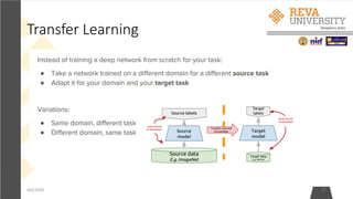
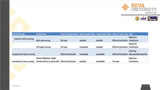
39. Practical advice for Transfer Learning
4/6/2020 39
• Constraints from pretrained models. Note that if you wish to use a pretrained network,
you may be slightly constrained in terms of the architecture you can use for your new
dataset. For example, you can't arbitrarily take out Conv layers from the pretrained
network. However, some changes are straight-forward: Due to parameter sharing, you
can easily run a pretrained network on images of different spatial size. This is clearly
evident in the case of Conv/Pool layers because their forward function is independent of
the input volume spatial size (as long as the strides "fit"). In case of FC layers, this still
holds true because FC layers can be converted to a Convolutional Layer: For example, in
an AlexNet, the final pooling volume before the first FC layer is of size [6x6x512].
Therefore, the FC layer looking at this volume is equivalent to having a Convolutional
Layer that has receptive field size 6x6, and is applied with padding of 0.
• Learning rates. It's common to use a smaller learning rate for ConvNet weights that are
being fine-tuned, in comparison to the (randomly-initialized) weights for the new linear
classifier that computes the class scores of your new dataset. This is because we expect
that the ConvNet weights are relatively good, so we don't wish to distort them too
quickly and too much (especially while the new Linear Classifier above them is being
trained from random initialization).

40. 4/6/2020 40

41. 4/6/2020 41

42. 4/6/2020 42

43. 4/6/2020 43
The key idea here is
to leverage the pre-
trained model’s
weighted layers to
extract features but
not to update the
weights of the
model’s layers during
training with new data
for the new task.

44. 4/6/2020 44

45. References
• https://ujjwalkarn.me/2016/08/11/intuitive-explanation-convnets/
• https://towardsdatascience.com/a-comprehensive-guide-to-convolutional-neural-networks-the-
eli5-way-3bd2b1164a53 #:~:text=A%20 Convolutional%20Neural %20Network%20
(ConvNet,differentiate%20one%20from%20the%20other.
• https://cs231n.github.io/convolutional-networks/
• https://machinelearningmastery.com/convolutional-layers-for-deep-learning-neural-networks/
• https://ujjwalkarn.me/2016/08/11/intuitive-explanation-convnets/
• https://ujjwalkarn.me/2016/08/09/quick-intro-neural-networks/
4/6/2020 45

46. Existing Models that can be leveraged for
your problems -
• For computer vision, you can leverage some popular models including,
• VGG-16
• VGG-19
• Inception V3
• XCeption
• ResNet-50
• For natural language processing
• Word2Vec
• GloVe
• FastText
• Universal Sentence Encoder by Google
• Bidirectional Encoder Representations from Transformers (BERT) by Google
4/6/2020 46

47. 478/1/2020