Downloaded 199 times

![APPENDIX
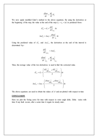
Matlab coding
clear
t = 0
tf=0
tfinal =0.5
tc=0.125
tstep=9.95
M=2.52/(180*50)
j=2
de1ta=21.64*pi/180
ddelta=0
time(1)=0
ang(1)=21.64
Pm=0.9
Pnaxbf=2.44
Pmaxdf=0.88
Pmaxaf=2.00
while t<tfinal,
if ( t==tf ),
Paminus=0.9-Pmaxbf*sin(delta)
Paplus=O.9-Pmaxdf*sine(delta)
Paav=(Paminus+Paplus)/2
Pa=Paav
end
if ( t==tc ) ,
Paminus=0.9-Pmaxdf*sin(delta)
Paplus=0.9-Pmaxaf*sin(delta)
Paav=(Paminus+Paplus)/2
Pa=Paav
end
if (t>tf & t<tc ),
Pa=Pm-Pmaxdf*sin(delta)
end
if (t>tc) ,
Pa=Pm-Pmaxaf*sin(delta)
end
t,Pa
ddelta=ddelta+(tstep*tstep*pa/M)
delta=(delta*180/pi+ddelta)*pi/180
deltadeg=det1a*180/Pi
t=t+tstep
pause
time(i)=t
ang(i)= deltadeg
ang(i)=deltadeg
i=i+1
end
axis([0 0.6 0 160])
plot(time,ang,'ko')](https://image.slidesharecdn.com/exp21-141101014712-conversion-gate01/85/Exp-2-1-2-To-plot-Swing-Curve-for-one-Machine-System-6-320.jpg)

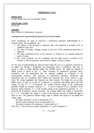
This document describes simulating the swing curve of a synchronous generator system. It provides the theory behind modeling a synchronous generator and defines the swing equation. It then gives an example problem of plotting the swing curve for a generator connected to an infinite bus when a fault occurs on one of the transmission lines. The document outlines the solving process using numerical integration methods to solve the swing equation and plot the rotor angle over time.