Downloaded 193 times
![Receiving End Power Circle
Diagram :14
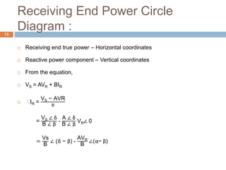
IR* =
|Vs|
|B|
∠ (β − δ ) -
|A||VR|
|B|
∠ (β − α)
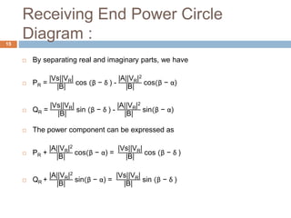
Volt- ampere at the receiving end will be
SR = PR + jQR = VR IR*
=
|Vs||VR|
|B|
∠ (β − δ ) -
|A||VR|2
|B|
∠(β − α)
=
|Vs||VR|
|B|
[cos (β − δ ) + j sin (β − δ )] -
|A||VR|2
|B|
[ cos(β − α)+j sin (β − δ )]
SR =
|Vs||VR|
|B|
cos (β − δ ) -
|A||VR|2
|B|
cos(β − α) +
|Vs||VR|
|B|
j sin (β − δ ) -
|A||VR|2
|B|
j sin (β − δ )](https://image.slidesharecdn.com/gp2-180222103939/85/Power-flow-through-transmission-line-14-320.jpg)

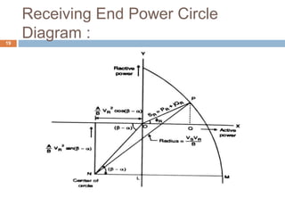
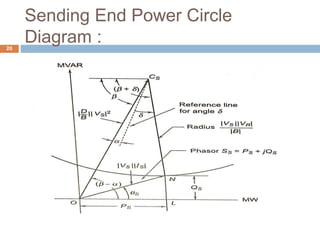
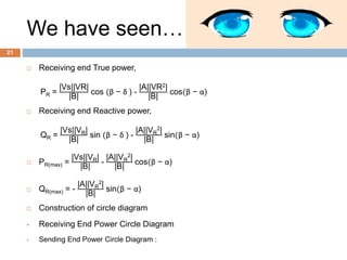


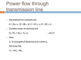
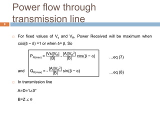
The document outlines power flow through transmission lines, detailing parameters such as inductance, capacitance, resistance, and conductance. It presents analytical and graphical methods for evaluating power flow, including the use of circle diagrams to represent true and reactive power at the receiving end. Key equations and methods for maximizing power transmission are also discussed.


