Load sharing between two interconnected power systems including transmission losses component

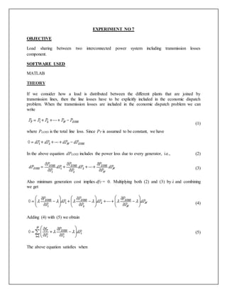
1. EXPERIMENT NO 7
OBJECTIVE
Load sharing between two interconnected power system including transmission losses
component.
SOFTWARE USED
MATLAB
THEORY
If we consider how a load is distributed between the different plants that are joined by
transmission lines, then the line losses have to be explicitly included in the economic dispatch
problem. When the transmission losses are included in the economic dispatch problem we can
write
where PLOSS is the total line loss. Since PT is assumed to be constant, we have
In the above equation dPLOSS includes the power loss due to every generator, i.e.,
Also minimum generation cost implies dfT = 0. Multiplying both (2) and (3) by λ and combining
we get
Adding (4) with (5) we obtain
The above equation satisfies when
(1)
(2)
(3)
(4)
(5)

2. (6)
Again since
from (6) we get
where Li is called the penalty factor of load- i and is given by
PROBLEM STATEMENT
A two-bus system is shown in figure below. If 100 Mw is transmitted from plant1 to the load, a
transmission loss of 10 MW is incurred. Find the required generation for each plant and the
power received by load when the system 휆 is Rs 25/MWh. The incremental fuel costs of the two
plants are given below
푑퐶1
푑푃 퐺1
= 0.020푃퐺1
+ 16 Rs/MWh
푑퐶2
푑푃 퐺2
= 0.04푃퐺2
+ 20 Rs/MWh
A two-bus system
(7)

3. CONCLUSION
The MATLAB code for the above problem is run and executed. It can be interpreted that the
minimum fuel cost is obtained, when the incremental fuel cost of each plant multiplied by its
penalty factor is the same for all the plants. Also when one generator is far away connected
through transmission line there is some loss component involved in that.
REFERENCES
[1]. Stevenson Jr, W. D. (1982). Elements of Power System Analysis, (4th), Mc-Graw Hill Higher
Education.
[2]. Hadi Saadat, “Power System Analysis”, Milwaukee School of Engineering, McGraw Hill,
1999.
[3]. Kothari D. P., Nagrath I. J., “Modern Power System Analysis”, Mc-Graw Hill Higher
Education.

4. APPENDIX
MATLAB CODE
clear
% MATLAB Program for optimum loading of generators
% This program finds the optimal loading of generators including
% penalty factors
% n is no of generators
n=2
% Pd stands for I oad demand
% alpha and beta arrays denote alpha beta coefficients for given
% generators
Pd = 237.04;
alpha=[ 0.020
0.04];
beta=[16
20];
lamda=20;
lamdaprev =lamda;
% tolerance is eps and increment in lamda is deltalamda
eps=1;
deltalamda = O.25;
% the minimum and maximum limits of each generating unit
% are stored in arrays Pgmin and Pgmax.
% In actual large scale problems,we can first initialise the Pgmax array
% to inf using for loop
% and Pgmin array to zero using Pgmin=zeros(n,1) command
PGmax=[200 200]:
Pgmin=[0 0] ;
B=[0.001 0
0 0] ;
Pg = zeros(n,1) ;
noofiter=0;
PL=0;
Pg = zeros(n,1);
while abs(sum(Pg)-PD-PL)>eps
for i=1:n
sigma=B(i,:)*Pg-B(i,i)*Pg(i) ;
Pg(i) =( 1-beta(i)/lamda-(2*sigma))/(alpha(i)/lamda+2*B(i,i));
PL=Pg'*B*Pg;
if Pg(i) > Pgmax(i)
Pg(i) =Pgmax(i) ;
end
if Pg(i) < Pgmin(i)
Pg(i) = Pgmin(i)
end

5. end
PL=Pg'*B*Pg;
if (sum(Pg)-Pd-PL) < 0
lamdaprev = lamda;
lamda=lamda+deltalamda;
else
lamdaprev=lamda;
lamda=lamda-deltalamda;
end
noofiter=noofiter+1 ;
Pg;
end
disp('The number of iterations required are')
noofiter
disp('The final value of lamda is')
lamdaprev
disp('The optimal loading of generators including penalty factors is')
Pg
disp('The losses are')
PL