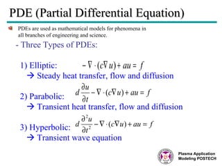
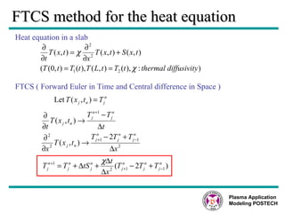
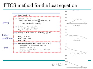
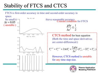
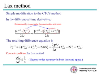
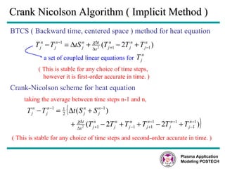
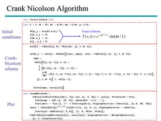
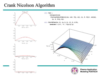
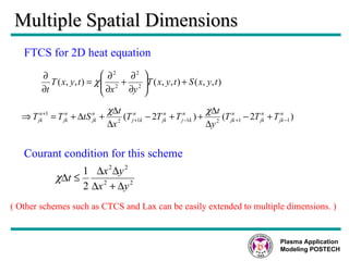
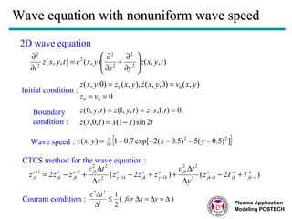
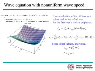
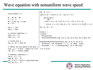
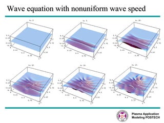
How to solve PDEs using  MATHEMATIA and MATLAB G. Y. Park, S. H. Lee and J.K. Lee Department of Electronic and Electrical Engineering, POSTECH 2006. 5. 17 Plasma Application Modeling POSTECH
Contents Solving PDEs using MATHEMATICA - FTCS method - Lax method - Crank Nicolson method - Jacobi’s method - Simultaneous-over-relaxation (SOR) method Solving PDEs using MATLAB - Examples of PDEs Plasma Application Modeling POSTECH
References Textbook - ‘Numerical and Analytical Methods for Scientists and Engineers Using Mathematica’, Daniel Dubin, Wiley, 2003 - ‘Applied numerical methods in C’, S. Nakamura Plasma Application Modeling POSTECH
PDE (Partial Differential Equation) PDEs are used as mathematical models for phenomena in  all branches of engineering and science. Plasma Application Modeling POSTECH - Three Types of PDEs: 1) Elliptic:     Steady heat transfer, flow and diffusion 2) Parabolic:    Transient heat transfer, flow and diffusion 3) Hyperbolic:    Transient wave equation
FTCS method for the heat equation FTCS ( Forward Euler in Time and Central difference in Space ) Heat equation in a slab Plasma Application Modeling POSTECH
FTCS method for the heat equation Initial  conditions Plot FTCS
Stability of FTCS and CTCS FTCS is first-order accuracy in time and second-order accuracy in space. So small time steps are required to achieve reasonable accuracy. CTCS method  for heat equation (Both the time and space derivatives are center-differenced.) However, CTCS method is   unstable   for  any  time step size. ( unstable ) Plasma Application Modeling POSTECH Courant condition  for FTCS
Lax method Simple modification to the CTCS method In the differenced time derivative, The resulting difference equation is ( Second-order accuracy in both time and space ) Plasma Application Modeling POSTECH Replacement by average value from surrounding grid points Courant condition  for Lax method
Crank Nicolson Algorithm ( Implicit Method ) BTCS ( Backward time, centered space ) method for heat equation ( This is stable for any choice of time steps, however it is first-order accurate in time. ) Crank-Nicolson scheme for heat equation taking the average between time steps n-1 and n, ( This is stable for any choice of time steps and second-order accurate in time. ) Plasma Application Modeling POSTECH a set of coupled linear equations for
Crank Nicolson Algorithm Initial  conditions Plot Crank-Nicolson scheme Exact solution
Crank Nicolson Algorithm Plasma Application Modeling POSTECH
Multiple Spatial Dimensions FTCS for 2D heat equation Courant condition for this scheme ( Other schemes such as CTCS and Lax can be easily extended to multiple dimensions. ) Plasma Application Modeling POSTECH
Wave equation with nonuniform wave speed 2D wave equation Initial condition : Boundary condition : Wave speed : CTCS method for the wave equation : Courant condition : Plasma Application Modeling POSTECH
Wave equation with nonuniform wave speed Since evaluation of the nth timestep refers back to the n-2nd step,  for the first step, a trick is employed. Since initial velocity and value, Plasma Application Modeling POSTECH
Wave equation with nonuniform wave speed Plasma Application Modeling POSTECH
2D Poisson’s equation Poisson’s equation Direct Solution for Poisson’s equation Centered-difference the spatial derivatives
Jacobi’s  method ( Relaxation method ) Direct solution can be difficult to program efficiently. Relaxation methods are relatively simple to code,  however, they are not as fast as the direct methods. Idea :   Poisson’s equation can be thought of as the equilibrium solution to the heat equation with source. Starting with any initial condition, the heat equation solution will eventually relax to a solution of Poisson’s equation. FTCS (Maximum time step satisfying Courant condition)
Jacobi method
Simultaneous OverRelaxation (SOR) The convergence of the Jacobi method is quite slow.  Furthermore, the larger the system, the slower the convergence. Simultaneous OverRelaxation (SOR) : the Jacobi method is modified in two ways, Improved values are used as soon as they become available. Relaxation parameter  ω  tries to overshoot for going to the final result. ( 1< ω <2) Plasma Application Modeling POSTECH
Simultaneous OverRelaxation (SOR)
O.V. Manuilenko MATLAB   The Language of Technical Computing MATLAB PDE Run:  dftcs.m >> dftcs dftcs - Program to solve the diffusion equation using the Forward Time Centered Space scheme. Enter time step: 0.0001 Enter the number of grid points: 51 Solution is expected to be stable Plasma Application Modeling Group POSTECH
O.V. Manuilenko MATLAB   The Language of Technical Computing MATLAB PDE Run:  dftcs.m >> dftcs dftcs - Program to solve the diffusion equation using the Forward Time Centered Space scheme. Enter time step: 0.00015 Enter the number of grid points: 61 WARNING:   Solution is expected to be unstable Plasma Application Modeling Group POSTECH
O.V. Manuilenko MATLAB   The Language of Technical Computing MATLAB PDE Run:  neutrn.m >>  neutrn Program to solve the neutron diffusion equation using the FTCS. Enter time step: 0.0005 Enter the number of grid points: 61 Enter system length: 2 =>  System length is subcritical Solution is expected to be stable Enter number of time steps: 12000 Plasma Application Modeling Group POSTECH
O.V. Manuilenko MATLAB   The Language of Technical Computing MATLAB PDE Run:  neutrn.m >>  neutrn Program to solve the neutron diffusion equation using the FTCS. Enter time step: 0.0005 Enter the number of grid points: 61 Enter system length: 4 =>  System length is supercritical Solution is expected to be stable Enter number of time steps: 12000 Plasma Application Modeling Group POSTECH
O.V. Manuilenko MATLAB   The Language of Technical Computing MATLAB PDE Run:  advect.m >> advect advect - Program to solve the advection equation using the various hyperbolic PDE schemes: FTCS, Lax, Lax-Wendorf Enter number of grid points: 50 Time for wave to move one grid spacing is 0.02 Enter time step: 0.002 Wave circles system in 500 steps Enter number of steps: 500 FTCS FTCS Plasma Application Modeling Group POSTECH
O.V. Manuilenko MATLAB   The Language of Technical Computing MATLAB PDE Run:  advect.m >> advect advect - Program to solve the advection equation using the various hyperbolic PDE schemes: FTCS, Lax, Lax-Wendorf Enter number of grid points: 50 Time for wave to move one grid spacing is 0.02 Enter time step: 0.02 Wave circles system in 50 steps Enter number of steps: 50 Lax Lax Plasma Application Modeling Group POSTECH
O.V. Manuilenko MATLAB   The Language of Technical Computing MATLAB PDE Run:  relax.m >> relax relax - Program to solve the Laplace equation using Jacobi, Gauss-Seidel and SOR methods on a square grid Enter number of grid points on a side: 50 Theoretical optimum omega = 1.88184  Enter desired omega: 1.8 Potential at y=L equals 1  Potential is zero on all other boundaries Desired fractional change = 0.0001 Plasma Application Modeling Group POSTECH

Finite DIfference Methods Mathematica

  • 1.
    How to solvePDEs using MATHEMATIA and MATLAB G. Y. Park, S. H. Lee and J.K. Lee Department of Electronic and Electrical Engineering, POSTECH 2006. 5. 17 Plasma Application Modeling POSTECH
  • 2.
    Contents Solving PDEsusing MATHEMATICA - FTCS method - Lax method - Crank Nicolson method - Jacobi’s method - Simultaneous-over-relaxation (SOR) method Solving PDEs using MATLAB - Examples of PDEs Plasma Application Modeling POSTECH
  • 3.
    References Textbook -‘Numerical and Analytical Methods for Scientists and Engineers Using Mathematica’, Daniel Dubin, Wiley, 2003 - ‘Applied numerical methods in C’, S. Nakamura Plasma Application Modeling POSTECH
  • 4.
    PDE (Partial DifferentialEquation) PDEs are used as mathematical models for phenomena in all branches of engineering and science. Plasma Application Modeling POSTECH - Three Types of PDEs: 1) Elliptic:  Steady heat transfer, flow and diffusion 2) Parabolic:  Transient heat transfer, flow and diffusion 3) Hyperbolic:  Transient wave equation
  • 5.
    FTCS method forthe heat equation FTCS ( Forward Euler in Time and Central difference in Space ) Heat equation in a slab Plasma Application Modeling POSTECH
  • 6.
    FTCS method forthe heat equation Initial conditions Plot FTCS
  • 7.
    Stability of FTCSand CTCS FTCS is first-order accuracy in time and second-order accuracy in space. So small time steps are required to achieve reasonable accuracy. CTCS method for heat equation (Both the time and space derivatives are center-differenced.) However, CTCS method is unstable for any time step size. ( unstable ) Plasma Application Modeling POSTECH Courant condition for FTCS
  • 8.
    Lax method Simplemodification to the CTCS method In the differenced time derivative, The resulting difference equation is ( Second-order accuracy in both time and space ) Plasma Application Modeling POSTECH Replacement by average value from surrounding grid points Courant condition for Lax method
  • 9.
    Crank Nicolson Algorithm( Implicit Method ) BTCS ( Backward time, centered space ) method for heat equation ( This is stable for any choice of time steps, however it is first-order accurate in time. ) Crank-Nicolson scheme for heat equation taking the average between time steps n-1 and n, ( This is stable for any choice of time steps and second-order accurate in time. ) Plasma Application Modeling POSTECH a set of coupled linear equations for
  • 10.
    Crank Nicolson AlgorithmInitial conditions Plot Crank-Nicolson scheme Exact solution
  • 11.
    Crank Nicolson AlgorithmPlasma Application Modeling POSTECH
  • 12.
    Multiple Spatial DimensionsFTCS for 2D heat equation Courant condition for this scheme ( Other schemes such as CTCS and Lax can be easily extended to multiple dimensions. ) Plasma Application Modeling POSTECH
  • 13.
    Wave equation withnonuniform wave speed 2D wave equation Initial condition : Boundary condition : Wave speed : CTCS method for the wave equation : Courant condition : Plasma Application Modeling POSTECH
  • 14.
    Wave equation withnonuniform wave speed Since evaluation of the nth timestep refers back to the n-2nd step, for the first step, a trick is employed. Since initial velocity and value, Plasma Application Modeling POSTECH
  • 15.
    Wave equation withnonuniform wave speed Plasma Application Modeling POSTECH
  • 16.
    Wave equation withnonuniform wave speed Plasma Application Modeling POSTECH
  • 17.
    2D Poisson’s equationPoisson’s equation Direct Solution for Poisson’s equation Centered-difference the spatial derivatives
  • 18.
    Jacobi’s method( Relaxation method ) Direct solution can be difficult to program efficiently. Relaxation methods are relatively simple to code, however, they are not as fast as the direct methods. Idea : Poisson’s equation can be thought of as the equilibrium solution to the heat equation with source. Starting with any initial condition, the heat equation solution will eventually relax to a solution of Poisson’s equation. FTCS (Maximum time step satisfying Courant condition)
  • 19.
  • 20.
    Simultaneous OverRelaxation (SOR)The convergence of the Jacobi method is quite slow. Furthermore, the larger the system, the slower the convergence. Simultaneous OverRelaxation (SOR) : the Jacobi method is modified in two ways, Improved values are used as soon as they become available. Relaxation parameter ω tries to overshoot for going to the final result. ( 1< ω <2) Plasma Application Modeling POSTECH
  • 21.
  • 22.
    O.V. Manuilenko MATLAB The Language of Technical Computing MATLAB PDE Run: dftcs.m >> dftcs dftcs - Program to solve the diffusion equation using the Forward Time Centered Space scheme. Enter time step: 0.0001 Enter the number of grid points: 51 Solution is expected to be stable Plasma Application Modeling Group POSTECH
  • 23.
    O.V. Manuilenko MATLAB The Language of Technical Computing MATLAB PDE Run: dftcs.m >> dftcs dftcs - Program to solve the diffusion equation using the Forward Time Centered Space scheme. Enter time step: 0.00015 Enter the number of grid points: 61 WARNING: Solution is expected to be unstable Plasma Application Modeling Group POSTECH
  • 24.
    O.V. Manuilenko MATLAB The Language of Technical Computing MATLAB PDE Run: neutrn.m >> neutrn Program to solve the neutron diffusion equation using the FTCS. Enter time step: 0.0005 Enter the number of grid points: 61 Enter system length: 2 => System length is subcritical Solution is expected to be stable Enter number of time steps: 12000 Plasma Application Modeling Group POSTECH
  • 25.
    O.V. Manuilenko MATLAB The Language of Technical Computing MATLAB PDE Run: neutrn.m >> neutrn Program to solve the neutron diffusion equation using the FTCS. Enter time step: 0.0005 Enter the number of grid points: 61 Enter system length: 4 => System length is supercritical Solution is expected to be stable Enter number of time steps: 12000 Plasma Application Modeling Group POSTECH
  • 26.
    O.V. Manuilenko MATLAB The Language of Technical Computing MATLAB PDE Run: advect.m >> advect advect - Program to solve the advection equation using the various hyperbolic PDE schemes: FTCS, Lax, Lax-Wendorf Enter number of grid points: 50 Time for wave to move one grid spacing is 0.02 Enter time step: 0.002 Wave circles system in 500 steps Enter number of steps: 500 FTCS FTCS Plasma Application Modeling Group POSTECH
  • 27.
    O.V. Manuilenko MATLAB The Language of Technical Computing MATLAB PDE Run: advect.m >> advect advect - Program to solve the advection equation using the various hyperbolic PDE schemes: FTCS, Lax, Lax-Wendorf Enter number of grid points: 50 Time for wave to move one grid spacing is 0.02 Enter time step: 0.02 Wave circles system in 50 steps Enter number of steps: 50 Lax Lax Plasma Application Modeling Group POSTECH
  • 28.
    O.V. Manuilenko MATLAB The Language of Technical Computing MATLAB PDE Run: relax.m >> relax relax - Program to solve the Laplace equation using Jacobi, Gauss-Seidel and SOR methods on a square grid Enter number of grid points on a side: 50 Theoretical optimum omega = 1.88184 Enter desired omega: 1.8 Potential at y=L equals 1 Potential is zero on all other boundaries Desired fractional change = 0.0001 Plasma Application Modeling Group POSTECH