Stability Stability Stability Stability Stability

Introduction Power System Stability
y y__
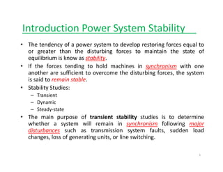
• The tendency of a power system to develop restoring forces equal to
or greater than the disturbing forces to maintain the state of
g g
equilibrium is know as stability.
• If the forces tending to hold machines in synchronism with one
another are sufficient to overcome the disturbing forces, the system
g , y
is said to remain stable.
• Stability Studies:
– Transient
Transient
– Dynamic
– Steady‐state
• The main purpose of transient stability studies is to determine
The main purpose of transient stability studies is to determine
whether a system will remain in synchronism following major
disturbances such as transmission system faults, sudden load
changes, loss of generating units, or line switching.
1

Introduction Power System Stability
y y__
• Transient Stability Problems:
– First‐swing; short study period after disturbance, based on a reasonable
First swing; short study period after disturbance, based on a reasonable
simple generator model, without control system.
– Multi‐swing; longer study period of time after disturbance, thus consider the
effect of generator control systems.
• In all stability studies, the objective is to determine whether or not the
rotors of the machines being perturbed return to constant speed
operation.
• To simplify calculation, the following assumptions must be made:
– Only synchronous frequency currents and voltages are considered in the
stator windings and the power system. Consequently dc offset currents and
harmonic components are neglected
harmonic components are neglected.
– Symmetrical components are used in the representation of unbalanced
faults.
– Generated voltage is considered unaffected by machine speed variation.
Generated voltage is considered unaffected by machine speed variation.
2

Rotor dynamics and the swing equation
y g q
• Accelerating torque is the product of the moment of inertia of
the rotor times its angular acceleration
the rotor times its angular acceleration.
e
m
a
m
T
T
T
d
J −
=
=
2
2
θ (14.1)
e
m
a
dt2
J the total moment of inertia of the rotor masses in kg m2
J the total moment of inertia of the rotor masses, in kg-m
m
θ the angular displacement of the rotor with respect to stationary axis, in mechanical radians
t time, in seconds
m
T the mechanical or shaft torque supplied by the prime mover less retarding torque due to rotational
m
losses, N-m
e
T the net electrical or electromagnetic torque, in N-m
a
T the net accelerating torque, in N-m
4

y g q
• The mechanical torque Tm and the electrical torque Te are considered
positive for the synchronous generator. Whereas for motor is another
way round.
• Tm is the resultant shaft torque that tends to accelerate the rotor in
the positive direction of rotation as shown in the figure.
• Under steady‐state operation of generator Tm and Te are equal and
l ti t T i
m
θ
accelerating torque Ta is zero.
• In this case there is no acceleration or deceleration of the rotor
masses and the resultant constant speed is the synchronous speed.
5

y g q
• is measured with respect to a stationary reference axis on the stator, it is
an absolute measure of rotor angle.
• Rotor angular position with respect to a reference axis which rotates at
m
θ
g p p
synchronous speed is given by:
m
sm
m t δ
ω
θ +
= (14.2)
• Where is the synchronous speed of the machine in mechanical radians
per second and is the angular displacement of the rotor, in mechanical
radians, from the synchronously rotating reference axis.
sm
ω
m
δ
• The derivatives of (14.2) with respect to time are:
d
d m
m δ
ω
θ
+
= (14.3)
dt
dt
sm
ω +
=
2
2
2
2
d
d
d
d m
m δ
θ
=
(14.3)
(14.4)
2
2
dt
dt
6

y g q
• Eq. (14.5) can be converted into power by multiplying with
angular velocity in Eq (14 6) (**Power = Torque x Angular
ω
angular velocity in Eq. (14.6) (**Power = Torque x Angular
velocity).
dt
d m
m
θ
ω =
(14.6)
m
ω
W
2
2
e
m
a
m
m P
P
P
dt
d
J −
=
=
δ
ω (14.7)
Where:
P the shaft power input to the machine less rotational losses
Pm the shaft power input to the machine less rotational losses
Pe the electrical power crossing its air gap
Pa the accelerating power which account for any unbalance between Pm and Pe
8

y g q
• Eq. (14.7) can also be written as in (14.8), whereby :
m
J
M ω
=
• M is inertia constant (joule‐seconds per mechanical radian)
W
2
2
e
m
a
m
P
P
P
dt
d
M −
=
=
δ (14.8)
• M is inertia constant (joule‐seconds per mechanical radian)
• In machine data supplied for stability studies, another constant
related to inertia is called H constant:
MVA
in
rating
machine
speed
s
synchronou
at
megajoules
in
energy
kinetic
stored
H =
(14.9)
MVA
MJ
S
M
S
J
H
mach
sm
mach
sm
/
2
1
2
1 2
ω
ω
=
=
MVA.
in
machine
the
of
rating
phase
three
the
−
mach
S
9

y g q
• Solving for M in Eq. (14.9);
rad
mech
MJ
S
H
M mach
sm
/
2
ω
= (14.10)
• Substitute the above equation in (14.8), we find;
P
P
P
d
H −
2
2 δ
mechanical radians
mechanical radians per seconds
• Eq. (14.11) can also be written as;
mach
e
m
mach
a
m
sm S
P
P
S
P
dt
d
H
=
=
2
2 δ
ω
(14.11)
perunit
P
P
P
dt
d
H
e
m
a
s
−
=
=
2
2
2 δ
ω
(14.12) Swing Equation
s
10

y g q
• For a system with an electrical frequency of f hertz, Eq. (14.12)
becomes ( in electrical radians)
δ
becomes ( in electrical radians)
(14.13)
perunit
P
P
P
dt
d
f
H
e
m
a −
=
=
2
2
δ
π
δ
• If in electrical degree
(14.14)
perunit
P
P
P
d
H
=
=
2
δ
δ
• Eq. (14.12) can be written as the
t fi t d diff ti l ti
(14.14)
perunit
P
P
P
dt
f
e
m
a −
=
=
2
180
perunit
P
P
P
dt
d
H
e
m
a
s
−
=
=
2
2
2 δ
ω
two first‐order differential equations:
perunit
P
P
d
d
H
e
m −
=
ω
2
s
dt
d
ω
ω
δ
−
=
(14.15) (14.16)
p
dt
e
m
s
ω dt
11

Further Considerations of the swing equation
g q
• In a stability study of a power system with many synchronous
machines only one MVA base common to all parts of the
machines, only one MVA base common to all parts of the
system can be chosen.
• Thus, H constant for each machine must be converted into per
unit base on common MVA base;
(14.17)
mach
h
t
S
H
H =
• The constant moment inertia M is rarely used in practice and H
(14.17)
system
mach
system
S
H
H
• The constant moment inertia M is rarely used in practice and H
is often used in stability study.
12

g q
• In a stability study for a large system with many machines
geographically dispersed over a wide area it is desirable to
geographically dispersed over a wide area, it is desirable to
minimize the number of swing equations to be solved.
• This can be done if the transmission line fault, or other
disturbance on the system, affects the machines within the
plant so that their rotors swing together.
• Thus the machine within the plant can be combined into a
• Thus, the machine within the plant can be combined into a
single equivalent machine just as if their rotors were
mechanically coupled and only one swing equation need to be
written for them.
13

g q
• Consider a power plant with two generators connected to the same
bus which is electrically remote from network disturbances the swing
bus which is electrically remote from network disturbances, the swing
equations on the common system base are:
perunit
P
P
dt
d
H
e
m 1
1
2
1
2
1
2
−
=
δ
ω
(14.18)
dt
s
ω
perunit
P
P
dt
d
H
e
m
s
2
2
2
2
2
2
2
−
=
δ
ω
(14.19)
• Adding the equation together, and denoting and by since the
rotor angle swing together;
1
δ 2
δ δ
d
H 2
2 δ
where
peruni
P
P
dt
d
H
e
m
s
−
=
2
2
2 δ
ω
(14.20)
2
1 H
H
H +
=
P
P
P
where 2
1
2
1 m
m
m P
P
P +
= 2
1 e
e
e P
P
P +
=
14

The Power‐Angle Equation
g q __________________
• In the swing equation, the input mechanical power from the
prime mover P is assumed constant
prime mover Pm is assumed constant.
• Thus, the Pe will determine whether the rotor accelerates,
Thus, the Pe will determine whether the rotor accelerates,
decelerates, or remains at synchronous speed.
• Changes in Pe are determined by conditions on the transmission
and distribution networks and the loads on the system to which
the generator supply power.
the generator supply power.
15

g q __________________
• Each synchronous machine is represented for transient stability
studies by its transient internal voltage E’ in series with the transient
y g
reactance X’d as shown in the Figure below.
• Armature resistance is negligible so that the phasor diagram is as
shown in the figure.
g
• Since each machine must be considered relative to the system, the
phasor angles of the machine quantities are measured with respect
to the common system reference.
y
+
jXd
'
I
E'
jIXd
'
Vt
_
E'
I
δ
α Vt
j d
Reference
(a) (b)
16

g q __________________
• Consider a generator supplying power through a transmission
system to a receiving end system at bus 2
system to a receiving‐end system at bus 2.
1
I 2
I E’1 is transient internal voltage of
generator at bus 1
'
1
E '
2
E
E’2 is transient internal voltage of
generator at bus 2
• The elements of the bus admittance matrix for the network
reduced to a two nodes in addition to the reference node is:
⎥
⎦
⎤
⎢
⎣
⎡
=
22
21
12
11
Y
Y
Y
Y
Ybas
(14.28)
17

g q __________________
• Power equation at a bus k is given by:
• Let k =1 and N=2 and substituting E’ for V
n
kn
N
n
k
k
k
V
Y
V
jQ
P
1
=
∗
∑
=
− (14.29)
• Let k =1 and N=2, and substituting E 2 for V,
( ) ( )∗
∗
+
=
+ '
2
12
'
1
'
1
11
'
1
1
1 E
Y
E
E
Y
E
jQ
P (14.30)
where
1
I 2
I
1
'
1
'
1 δ
∠
= E
E 2
'
2
'
2 δ
∠
= E
E
11
11
11 jB
G
Y +
= 12
12
12 θ
∠
= Y
Y
'
1
E '
2
E
18

g q __________________
• We obtain:
2
)
(
cos 12
2
1
12
'
2
'
1
11
2
'
1
1 θ
δ
δ −
−
+
= Y
E
E
G
E
P
)
(
sin 12
2
1
12
'
2
'
1
11
2
'
1
1 θ
δ
δ −
−
+
−
= Y
E
E
B
E
Q
(14.31)
(14.32)
• If we let and , we obtain from (14.31) and
(14.32)
2
1 δ
δ
δ −
=
2
12
π
θ
γ −
=
)
-
(
sin
12
'
2
'
1
11
2
'
1
1 γ
δ
Y
E
E
G
E
P +
=
2
(14.33)
)
-
(
cos
12
'
2
'
1
11
2
'
1
1 γ
δ
Y
E
E
B
E
Q −
−
= (14.34)
19

g q __________________
• Eq. (14.33) can be written more simply as
where
(14.35)
)
sin(
max γ
δ −
+
= P
P
P c
e
• When the network is considered without resistance, all the
elements of Y are susceptances so both G and becomes
(14.36)
11
2
'
1 G
E
Pc = 12
'
2
'
1
max Y
E
E
P =
γ
elements of Ybus are susceptances, so both G11 and becomes
zero and Eq. (14.35) becomes;
δ
sin
max
P
Pe = (14.37) Power Angle Equation
γ
where , with X is the transfer reactance between
E’1 and E’2
max
e
X
E
E
P '
2
'
1
max =
1 2
20

Example 1: Power‐angle equation before fault
p g q
The single‐line diagram shows a generator connected through parallel
transmission lines to a large metropolitan system considered as an infinite
bus. The machine is delivering 1.0 pu power and both the terminal voltage
and the infinite‐bus voltage are 1.0 pu. The reactance of the line is shown
based on a common system base. The transient reactance of the generator is
0 20 pu as indicated Determine the power‐angle equation for the system
0.20 pu as indicated. Determine the power‐angle equation for the system
applicable to the operating conditions.
21

p g q
The reactance diagram for the system is shown:
The series reactance between the terminal voltage (Vt) and the infinite bus is:
unit
per
3
.
0
2
4
.
0
10
.
0 =
+
=
X
The series reactance between the terminal voltage (Vt) and the infinite bus is:
The 1.0 per unit power output of the generator is determined by the power‐angle
1.0
sin
3
.
0
(1.0)(1.0)
sin =
= α
α
X
V
Vt
The 1.0 per unit power output of the generator is determined by the power angle
equation.
α
V is the voltage of the infinite bus, and is the angle of the terminal voltage
relative to the infinite bus
22

p g q
Solve α
0
1 0
1
458
.
17
3
.
0
sin =
= −
α
Terminal voltage, Vt : unit
per
300
.
0
954
.
0
458
.
17
0
.
1 0
j
Vt +
=
∠
=
The output current from the generator is:
3
0
0
0
.
1
458
.
17
0
.
1 0
0
j
I
∠
−
∠
= unit
per
729
.
8
012
.
1
1535
.
0
0
.
1 0
∠
=
+
= j
3
.
0
j
p
j
The transient internal voltage is
XI
V
E +
=
' XI
V
E t +
=
)
1535
.
0
0
.
1
)(
2
.
0
(
)
30
.
0
954
.
0
(
' j
j
j
E +
+
+
=
unit
per
44
.
28
050
.
1
5
.
0
923
.
0 0
∠
=
+
= j
23

p g q
The power‐angle equation relating the transient internal voltage E’ and the
infinite bus voltage V is determined by the total series reactance
infinite bus voltage V is determined by the total series reactance
unit
per
5
.
0
2
4
.
0
1
.
0
2
.
0 =
+
+
=
X
Hence, the power‐angle equation is:
u
p
Pe .
sin
1
.
2
sin
5
0
)
0
.
1
)(
05
.
1
(
δ
δ =
=
5
.
0
δ
Where is the machine rotor angle with respect to infinite bus
The swing equation for the machine is
The swing equation for the machine is
unit
per
sin
10
.
2
0
.
1
180 2
2
δ
δ
−
=
dt
d
f
H
H is in megajoules per megavoltampere, f is the electrical frequency of the system
and is in electrical degree
δ
24

Example 1: Power‐angle equation
p g q
The power‐angle equation is plotted:
Before fault
After fault
During fault
25

Example 2: Power‐angle equation During Fault
p g q g
The same network in example 1 is used. Three phase fault
occurs at point P as shown in the Figure Determine the power
occurs at point P as shown in the Figure. Determine the power‐
angle equation for the system with the fault and the
corresponding swing equation. Take H = 5 MJ/MVA
26

p g q g
Approach 1:
Th di f h d i f l i h b l
The reactance diagram of the system during fault is shown below:
The value is admittance
per unit
p
27

p g q g
As been calculated in example 1, internal transient voltage remains
as (based on the assumption that flux linkage is
°
∠
= 44
28
05
1
'
E
The Y bus is:
as (based on the assumption that flux linkage is
constant in the machine)
∠ 44
.
28
05
.
1
E
⎥
⎥
⎤
⎢
⎢
⎡
−
−
= 50
2
50
7
0
333
.
3
0
333
.
3
j
Yb
⎥
⎥
⎦
⎢
⎢
⎣ − 833
.
10
50
.
2
333
.
3
50
.
2
50
.
7
0
j
Ybas
Since bus 3 has no external source connection and it may be removed by the node
li i ti d th Y b t i i d d t
elimination procedure, the Y bus matrix is reduced to:
[ ]
5
.
2
333
.
3
833
10
1
5
2
333
.
3
5
7
0
0
333
.
3
⎥
⎦
⎤
⎢
⎣
⎡
−
⎥
⎦
⎤
⎢
⎣
⎡−
=
bus
Y
833
.
10
5
.
2
5
.
7
0 −
⎥
⎦
⎢
⎣
⎥
⎦
⎢
⎣ −
⎥
⎤
⎢
⎡−
=
⎥
⎤
⎢
⎡ 769
.
0
308
.
2
12
11
j
Y
Y
⎥
⎦
⎢
⎣ −
⎥
⎦
⎢
⎣ 923
.
6
769
.
0
22
21
j
Y
Y
28

p g q g
The magnitude of the transfer admittance is 0.769 and therefore,
The power‐angle equation with the fault on the system is therefore,
' ' '
max 1 2 12 (1.05)(1.0)(0.769) 0.808
P E E Y per unit
= = =
unit
per
sin
808
.
0 δ
=
e
P
The corresponding swing equation is
The corresponding swing equation is
5
180
10 0808
2
2
f
d
dt
δ
δ
= −
. . sin per unit
Because of the inertia, the rotor cannot change position instantly upon
occurrence of the fault. Therefore, the rotor angle is initially 28.440 and
the electrical power output is
δ
385
0
44
28
i
808
0 °
P 385
.
0
44
.
28
sin
808
.
0 =
°
=
e
P
29

p g q g
The initial accelerating power is: Pa = − =
10 0385 0615
. . . per unit
and the initial acceleration is positive with the value given by
d
dt
f
f
2
2
180
5
0615 2214
δ
= =
( . ) . elec deg / s2
30

p g q g
Approach 2:
C h d li ( hi h i Y f ) i d l d
Covert the read line (which in Y form) into delta to remove node
3 from the network:
j1.3
1
1
3
1
1 3
3
2
2
3
1
)
4
.
0
)(
2
.
0
(
)
4
.
0
)(
3
.
0
(
)
2
.
0
)(
3
.
0
( j
j
j
j
j
j
R
+
+
j0.65 j0.8667
3
.
1
2
.
0
)
4
.
0
)(
2
.
0
(
)
4
.
0
)(
3
.
0
(
)
2
.
0
)(
3
.
0
(
j
j
j
j
j
j
j
j
RAC =
+
+
=
65
.
0
4
.
0
)
4
.
0
)(
2
.
0
(
)
4
.
0
)(
3
.
0
(
)
2
.
0
)(
3
.
0
(
j
j
j
j
j
j
j
j
RAB =
+
+
=
31
8667
.
0
3
.
0
)
4
.
0
)(
2
.
0
(
)
4
.
0
)(
3
.
0
(
)
2
.
0
)(
3
.
0
(
j
j
j
j
j
j
j
j
RBC =
+
+
=

p g q g
Approach 2:
Covert the read line which in Y form into delta to remove node
Covert the read line, which in Y form into delta to remove node
3 from the network:
j0.1625
769
.
0
)
3
.
1
/
1
(
12 =
−
= j
Y
12
'
2
'
1 Y
E
E
P = )
(
12 j
max (1.05)(1.0)(0.769) 0.808
0.808sin
e
P
P δ
= =
=
12
2
1
max Y
E
E
P
32
e

Example 3: Power‐angle equation After Fault Cleared
p g q
The fault on the system cleared by simultaneous opening of
the circuit breakers at each end of the affected line
the circuit breakers at each end of the affected line.
Determine the power‐angle equation and the swing
equation for the post‐fault period
CB open CB open
33

Example 3: Power‐angle equation After Fault Cleared
p g q
Upon removal of the faulted line, the net transfer admittance
across the system is
across the system is
y
j
j
12
1
0 2 01 0 4
1429
=
+ +
= −
( . . . )
. per unit 429
.
1
12 j
Y =
or
The post‐fault power‐angle equation is
δ
δ sin
5
.
1
sin
)
429
.
1
(
)
0
.
1
(
)
05
.
1
( =
=
e
P )
(
)
(
)
(
e
and the swing equation is
5
180
10 1500
2
2
f
d
dt
δ
δ
= −
. . sin
34

Synchronizing Power Coefficients___________
• From the power‐angle
curve, two values of angle
satisfied the mechanical
Before fault
satisfied the mechanical
power i.e at 28.440 and
151.560.
H l th 28 440 After fault
• However, only the 28.440
is acceptable operating
point.
A t bl ti
• Acceptable operating
point is that the
generator shall not lose
synchronism when small
During fault
synchronism when small
temporary changes occur
in the electrical power
output from the machine
output from the machine.
35

Consider small incremental changes in the operating point parameters, that is:
Δ
+
= δ
δ
δ 0
Δ
+
= e
e
e P
P
P 0
(14.40)
Substituting above equation into Eq 14 37 (Power angle equation) δ
sin
P
P =
Substituting above equation into Eq. 14.37 (Power‐angle equation)
)
sin
cos
cos
(sin
)
sin(
0
0
max
0
max
0
Δ
Δ
Δ
Δ
+
=
+
=
+
δ
δ
δ
δ
δ
δ
P
P
P
P e
e
δ
sin
max
P
Pe =
)
s
cos
cos
(s 0
0
max Δ
Δ δ
δ
δ
δ
(14.41)
Since is a small incremental displacement from
Δ
δ
0
δ
Δ
Δ ≅ δ
δ
sin 1
cos ≅
Δ
δ
Thus, the previous equation becomes:
+
=
+ δ
δ
δ )
cos
(
sin P
P
P
P
(14.42)
Δ
Δ +
=
+ δ
δ
δ )
cos
(
sin 0
max
0
max
0 P
P
P
P e
e
36

At the initial operating point :
0
δ
sinδ
P
P
P =
= (14 43)
0
max
0 sinδ
P
P
P e
m =
= (14.43)
Equation (14.42) becomes:
(14 44)
Δ
Δ −
=
+
− δ
δ )
cos
(
)
( 0
max
0 P
P
P
P e
e
m
(14.44)
Substitute Eq. (14.40) into swing equation;
)
(
)
(
2
0
2
0
2
Δ
Δ
+
−
=
+
e
e
m
s
P
P
P
dt
d
H δ
δ
ω
(14.45)
Replacing the right‐hand side of this equation by (14.44);
0
)
cos
(
2
0
max
2
2
=
+ Δ
Δ
δ
δ
δ
P
d
d
H
(14.46)
)
( 0
max
2 Δ
ω dt
s
37

Since is a constant value. Noting that is the slope of the power‐
angle curve at the angle , we denote this slope as Sp and define it as:
0
δ 0
max cosδ
P
0
δ
(14.47)
0
max cos
0
δ
δ δ
δ
P
d
dP
S e
p =
=
=
Where Sp is called the synchronizing power coefficient. Replacing Eq. (14.47) into (14.46);
0
2
Δ
δ
ω
δ S
d p
s (14 48)
0
2
2
=
+ Δ
Δ
δ
δ
H
dt
d p
s (14.48)
The above equation is a linear, second‐order differential equation.
If Sp positive – the solution corresponds to that of simple harmonic motion.
If Sp negative – the solution increases exponentially without limit.
)
(t
Δ
δ
)
(t
Δ
δ
p g p y
)
(t
Δ
δ
38

The angular frequency of the un‐damped oscillations is given by:
s
rad
elec
H
Sp
s
n /
2
ω
ω =
(14.49)
which corresponds to a frequency of oscillation given by:
H
S
f
p
s
1 ω
(14.50)
Hz
H
f
p
s
n
2
2
1
π
=
39

Example:
The machine in previous example is operating at when it is subjected
to a slight temporary electrical‐system disturbance. Determine the frequency
°
= 44
.
28
δ
to a slight temporary electrical system disturbance. Determine the frequency
and period of oscillation of the machine rotor if the disturbance is removed
before the prime mover responds. H = 5 MJ/MVA.
8466
.
1
44
.
28
cos
10
.
2 =
°
=
p
S
The synchronizing power coefficient is
The angular frequency of oscillation is therefore;
s
rad
elec
H
S p
s
n /
343
.
8
5
2
8466
.
1
377
2
=
×
×
=
=
ω
ω
343
8
The corresponding frequency of oscillation is Hz
fn 33
.
1
2
343
.
8
=
=
π
and the period of oscillation is s
f
T
n
753
.
0
1
=
=
fn
40

Equal‐Area Criterion of Stability______________
The swing equation is non‐linear in nature and thus, formal solution
cannot be explicitly found.
cannot be explicitly found.
perunit
P
P
P
dt
d
H
e
m
a −
=
=
2
2
2 δ
ω
To examine the stability of a two‐machine system without solving the
dt
s
ω
swing equation, a direct approach is possible to be used i.e using equal‐
area criterion.
41

Consider the following system:
At point P (close to the bus), a three‐phase fault occurs and cleared by circuit
breaker A after a short period of time.
Thus, the effective transmission system is unaltered except while the fault is on.
The short‐circuit caused by the fault is effectively at the bus and so the
The short circuit caused by the fault is effectively at the bus and so the
electrical power output from the generator becomes zero until fault is clear.
42
three‐phase fault

To understand the physical condition before, during and after the fault,
power‐angle curve need to be analyzed.
Initially, generator operates at synchronous speed with rotor angle of
and the input mechanical power equals the output electrical power Pe.
0
δ
Before fault, Pm = Pe
43

At t = 0, Pe = 0, Pm = 1.0 pu
Acceleration constant
The difference must be accounted for by a
rate of change of stored kinetic energy in
the rotor masses.
Speed increase due to the drop of Pe
constant acceleration from t = 0 to t = tc. 1.0 pu
For t<tc, the acceleration is constant given
by:
perunit
P
d
H
0
2
−
=
ω
At t = 0, three phase fault occurs
d
P
s
2
2
δ ω
= (14.51)
perunit
P
dt
m
s
0
=
ω
dt H
Pm
2
2
(14.51)
44

While the fault is on, velocity increase
above synchronous speed and can be
above synchronous speed and can be
found by integrating this equation:
d t
δ ω ω
∫
d
dt H
P dt
H
P t
s
m
s
m
t
δ ω ω
= =
∫ 2 2
0
For rotor angular position,;
(14.52)
δ
ω
δ
+
s m
P
t2 (14.53)
δ δ
= +
s m
H
t
4
2
0
(14.53)
(14.52) 45

Eq. (14.52) & (14.53) show that the
velocity of the rotor increase linearly
velocity of the rotor increase linearly
with time with angle move from to
0
δ c
δ
At the instant of fault clearing t = tc,
g ,
the increase in rotor speed is
d P
s m
δ ω
dt H
t
t t
s m
c
c
= =
2
angle separation between the generator
and the infinite bus is
(14.54)
and the infinite bus is
( )
δ
ω
δ
t
P
H
t
t t
s m
c
c
= = +
4
2
0
(14.55)
(14.52) 46

When fault is cleared at , Pe
increase abruptly to point d
c
δ
At d, Pe > Pm , thus Pa is
negative
Rotor slow down as P goes
Rotor slow down as Pe goes
from d to e
At t = tc, fault is cleared
47

1. At e, the rotor speed is again
synchronous although rotor angle has
advance to x
δ
2. The angle is determined by the
fact that A1 = A2
x
δ
x
3. The acceleration power at e is still
negative (retarding), so the rotor
cannot remain at synchronous speed
but continue to slow down.
4. The relative velocity is negative and
the rotor angle moves back from point
the rotor angle moves back from point
e to point a, which the rotor speed is
less than synchronous.
6 In the absence of damping rotor would
5. From a to f, the Pm exceeds the Pe
and the rotor increase speed again until
reaches synchronous speed at f
6. In the absence of damping, rotor would
continue to oscillate in the sequence f‐a‐e, e‐a‐
f, etc 48

In a system where one machine is swinging with respect to infinite bus,
equal‐area criterion can be used to determine the stability of the system
d i di i b l i i i
under transient condition by solving swing equation.
Equal‐area criterion not applicable for multi‐machines.
The swing equation for the machine connected to the infinite bus is
d
H 2
2 δ
(14.56)
e
m
s
P
P
dt
d
H
−
=
2
2
2 δ
ω
Define the angular velocity of the rotor relative to synchronous speed by
ω
δ
ω ω
r s
d
dt
= = − (14.57)
s
dt
49

Differentiate (14.57) with respect to t and substitute in (14.56) ;
(14.58)
2H d
dt
P P
s
r
m e
ω
ω
= −
When rotor speed is synchronous, equals and is zero.
ω s
ω r
ω
Multiplying both side of Eq. (14.58) by ;
dt
d
r /
δ
ω =
H d d
ω δ
( )
H d
dt
P P
d
dt
s
r
r
m e
ω
ω
ω δ
2 = − (14.59)
The left‐hand side of the Eq. can be rewritten to give
(14.60)
dt
d
P
P
dt
d
H
e
m
r
s
δ
ω
ω
)
(
)
(
2
−
=
50

Multiplying by dt and integrating, we obtain;
δ
(14.61)
∫ −
=
−
2
1
)
(
)
( 2
1
2
2
δ
δ
δ
ω
ω
ω
d
P
P
H
e
m
r
r
s
Since the rotor speed is synchronous at and then ;
δ δ 0
=
= ω
ω
Since the rotor speed is synchronous at and , then ;
1
δ 2
δ 0
2
1 =
= r
r ω
ω
Under this condition, (14.61) becomes
(14.59)
( )
P P d
m e
− =
∫ δ
δ
δ
0
1
2
and are any points on the power angle diagram provided that there are
points at which the rotor speed is synchronous.
1
δ 2
δ
51

In the figure, point a and e correspond to and
1
δ 2
δ
If perform integration in two steps;
If perform integration, in two steps;
0
)
(
)
(
0
=
−
+
− ∫
∫ δ
δ
δ
δ
δ
δ
d
P
P
d
P
P
x
c
c
e
m
e
m
(14.63)
δ
δ
δ
δ
δ
δ
d
P
P
d
P
P
x
c
c
m
e
e
m ∫
∫ −
=
− )
(
)
(
0
(14.64)
Fault period
Area A1
Post‐fault period
Area A2
The area under A1 and A4 are directly proportional to
the increase in kinetic energy of the rotor while it is
accelerating.
The area under A and A are directly proportional to
the decrease in kinetic energy of the rotor while it is
decelerating. 52

Equal‐area criterion states that whatever kinetic energy is added to the
rotor following a fault must be removed after the fault to restore the rotor
to synchronous speed
to synchronous speed.
The shaded area A1 is dependent upon the time taken to
clear the fault.
If the clearing has a delay, the angle increase.
As a result, the area A2 will also increase. If the increase
c
δ
As a result, the area A2 will also increase. If the increase
cause the rotor angle swing beyond , then the rotor
speed at that point on the power angle curve is above
synchronous speed when positive accelerating power is
i t d
max
δ
again encountered.
Under influence of this positive accelerating power the
angle will increase without limit and instability results.
g y
53

There is a critical angle for clearing the fault in order to satisfy the
requirements of the equal‐area criterion for stability.
This angle is called the critical clearing angle
The corresponding critical time for removing the fault is called critical
cr
δ
The corresponding critical time for removing the fault is called critical
clearing time tcr
Power‐angle curve showing the
critical‐clearing angle . Area A1
and A2 are equal
cr
δ
54

The critical clearing angle and critical clearing time tcr can be calculated
by calculating the area of A1 and A2.
cr
δ
( )
A P d P
m m cr
cr
1 0
0
= = −
∫ δ δ δ
δ
δ
( )
∫
δ
(14.65)
(14 66)
( )
A P P d
m
cr
2 = −
∫ max sin
max
δ δ
δ
δ
)
(
)
cos
(cos max
max
max cr
m
cr P
P δ
δ
δ
δ −
−
−
=
(14.66)
)
(
)
( max
max
max cr
m
cr
Equating the expressions for A1 and A2, and transposing terms, yields
( )( )
/
δ δ δ δ
P P + (14.67)
( )( )
cos / cos
max max max
δ δ δ δ
cr m
P P
= − +
0
55

From sinusoidal power‐angle curve, we see that
(14 68)
δ π δ elec rad (14.68)
δ π δ
max = − 0 elec rad
P P
m = max sinδ0
(14.69)
Substitute and in Eq. (14.67),
simplifying the result and solving for
max
δ max
P
cr
δ
( )
[ ]
δ π δ δ δ
= −
cos sin cos
1
2 (14 70)
( )
[ ]
δ π δ δ δ
cr = − −
cos sin cos
0 0 0
2 (14.70)
In order to get tcr, substitute critical angle equation into (14.55) and then solve to
obtain tcr;
δ
ω
δ
cr
s m
cr
P
H
t
= +
4
2
0
( )
t
H
P
cr
cr
s m
=
−
4 0
δ δ
ω
(14.71) (14.72)
56

Equal‐Area Criterion of Stability ‐Example_____
Calculate the critical clearing angle and critical clearing time for the system shown
below. When a three phase fault occurs at point P. The initial conditions are the
same as in Example 1 and H = 5MJ/MVA
p /
P P
e = =
max sin . sin
δ δ
210
Solution
The power angle equation is
The initial rotor angle is
δ0
0
28 44 0 496
= =
. . elec rad
d h h l h f h l l
and the mechanical input power Pm is 1.0 pu. Therefore, the critical angle is
calculated using Eq. (14.70)
( )
[ ]
δ π
cr = − × −
−
cos . sin . cos .
1 0 0
2 0 496 28 44 28 44 = =
81697 1426
0
. . elec rad
( )
[ ]
δ π δ δ δ
cr = − −
−
cos sin cos
1
0 0 0
2
and the critical clearing time is
( )
× −
4 5 1426 0496
. . = 0 222s
( )
tcr =
×
377 1
= 0.222s
57

Further Application of the Equal‐Area Criterion
• Equal‐Area Criterion can only be applied for
the case of two machines or one machine
and infinite bus
and infinite bus.
• When a generator is supplying power to an
infinite bus over two parallel lines, opening
one of the lines may cause the generator to
lose synchronism
lose synchronism.
• If a three phase fault occurs on the bus on
which two parallel lines are connected, no
power can be transmitted over either the
line
line.
• If the fault is at the end of one of the lines, CB will operate and power can
flow through another line.
• In this condition, there is some impedance between the parallel buses and
the fault. Thus, some power is transmitted during the fault.
58

Further Application of the Equal‐Area Criterion
Considering the transmitted of power during fault, a general Equal‐area
criterion is applied;
criterion is applied;
By evaluating the area A1 and A2 as in the previous approach, we can find that;
1
max
2
max
max cos
cos
)
)(
/
(
cos
r
r
P
P o
o
m
cr
−
+
−
=
δ
δ
δ
δ
δ (14.73)
1
2 r
r
cr
−
( )
59

Further Application of the Equal‐Area Criterion ‐ Example
Determine the critical clearing angle for the three phase fault described in the
previous example.
The power‐angle equations obtained in the previous examples are
The power‐angle equations obtained in the previous examples are
δ
δ sin
1
.
2
sin
max =
P δ
δ sin
808
.
0
sin
max
1 =
P
r
δ
δ sin
5
.
1
sin
max
2 =
P
r
Before fault: During fault:
After fault:
Hence
385
.
0
1
.
2
808
.
0
1 =
=
r 714
.
0
1
.
2
5
.
1
2 =
=
r
rad
412
.
2
19
.
138
5
.
1
0
.
1
sin
180 1
max =
°
=
−
°
= −
δ
)
44
.
28
cos(
385
.
0
)
19
.
138
cos(
714
.
0
)
496
.
0
412
.
2
)(
1
.
2
/
0
.
1
(
cos
°
−
°
+
−
δ
127
.
0
385
.
0
714
.
0
)
(
)
(
)
)(
(
cos
=
−
=
cr
δ
°
= 726
.
82
cr
δ
To determine the critical clearing time, we must obtain the swing curve of
versus t for this example.
δ
60

STEP‐BY‐STEP SOLUTION OF SWING CURVE____
For large systems we depend on the digital computer to determine δ versus t
for all the machines in which we are interested; and δ can be plotted versus t
for all the machines in which we are interested; and δ can be plotted versus t
for a machines to obtain the swing curve of that machine.
The angle δ is calculated as a function of time over a period long enough to
g p g g
determine whether δ will increase without limit or reach a maximum and
start to decrease.
Although the latter result usually indicates stability, on an actual system
where a number of variable are taken into account it may be necessary to plot
δ versus t over a long enough interval to be sure δ will not increase again
ith t t i t l l
without returning to a low value.
61

By determining swing curves for various clearing times the length of time
permitted before clearing a fault can be determined.
Standard interrupting times for circuit breakers and their associated relays
are commonly 8, 5, 3 or 2 cycles after a fault occurs, and thus breaker
speeds may be specified.
Calculations should be made for a fault in the position which will allow the
least transfer of power from the machine and for the most severe type of
fault for which protection against loss of stability is justified.
A number of different methods are available for the numerical evaluation
of second order differential equations in step by step computations for
of second‐order differential equations in step‐by‐step computations for
small increments of the independent variable.
The more elaborate methods are practical only when the computations are
62
The more elaborate methods are practical only when the computations are
performed on a digital computer. The step‐by‐step method used for hand
calculation is necessarily simpler than some of the methods recommended
for digital computers.

In the method for hand calculation the change in the angular position of the
rotor during a short interval of time is computed by making the following
assumptions:
assumptions:
•The accelerating power Pa computed at the beginning of an interval is
constant from the middle of the preceding interval to the middle of the
constant from the middle of the preceding interval to the middle of the
interval considered.
•The angular velocity is constant throughout any interval at the value
g y g y
computed for the idle of the interval.
**neither of the assumptions is true, since δ is changing continuously and both Pa
and ω are functions of δ.
63
As the time interval is decreased, the computed swing curve approaches the true
curve.

and
Figure 14.4 will help in visualizing the assumptions.
The accelerating power is computed for the points
The accelerating power is computed for the points
enclosed in circles at the ends of the n-2, n-1, and n
intervals, which are the beginnings of the n-1, n and
n+1 interval.
The step curve of Pa in Fig. 14.4 results from the
assumption that Pa is constant between midpoints of
the intervals.
Similarly, ωr, the excess of the angular velocity ω
over the synchronous angular velocity ωs, is shown
as a step curve that is constant throughout the
interval at the value computed for the midpoint.
e v e v ue co pu ed o e dpo .
Between the ordinates (n-3/2) and (n-1/2) there
64
Between the ordinates (n 3/2) and (n 1/2) there
is a change of speed caused by the constant
accelerating power.

The change in speed in the product of the
acceleration and the time interval, thus:
ω ω
δ
r n r n a n
d
dt
t
f
H
P t
, / , / ,
1 2 3 2
2
2 1
180
− = = −
Δ Δ (1)
The change in δ over any interval is the
product of ω, for the interval and the time of
the interval. Thus, the change in δ during the
1 i l i
n‐1 interval is:
Δ Δ
δ δ δ ω
n n n r n
t
− − − −
= − =
1 1 2 3 2
, /
(2)
and during the nth interval
65
Δ Δ
δ δ δ ω
n n n r n
t
= − =
− −
1 1 2
, /
(3)
Fig. 14.14

Substracting Eq (2) from Eq. (3) and
substituting Eq. (1) in the resulting
equation to eliminate all values of ω,
(4)
yields
Δ Δ
δ δ
n n a n
kP
= +
− −
1 1
,
where
( )
k
f
t
=
180 2
Δ
(5)
( )
H
66
Fig. 14.14

Equation (4) is the important for the step-by-step solution of the swing equation with the necessary
assumption enumerated, for it shows how to calculate the change in δ for the previous interval and
the accelerating power for the interval in equation are known.
Equation (4) shows that (subject to the stated assumptions), the change in torque angle during a
given interval is equal to the change in torque angle during the preceding interval plus the
accelerating power at the beginning of the interval times k.
The accelerating power is calculated at the beginning of each new interval. The solution progresses
through enough intervals to obtain points for plotting the swing curve.
Greater accuracy is obtained when the duration of the interval is small. An interval of 0.05s is
y
usually satisfactory.
The occurrence of a fault causes a discontinuity in the accelerating power Pa which is zero before
the fault and a definite amount immediately following the fault.
y g
The discontinuity occurs at the beginning of the interval, when t=0. Reference to Fig. 14.14 shows
that our method of calculation assumes that the accelerating power computed at the beginning of an
interval considered.
67
When the fault occurs, we have two values of Pa at the beginning of the interval, and we must take
the average of these two values as our constant accelerating power.

Stability Stability Stability Stability Stability

Recommended

Recommended

More Related Content

Similar to Stability Stability Stability Stability Stability

Similar to Stability Stability Stability Stability Stability (20)

Recently uploaded

Recently uploaded (20)

Stability Stability Stability Stability Stability