Downloaded 46 times

![Unit-IV Finite Difference and Interpolation
Rai University | Ahmedabad
3
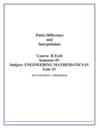
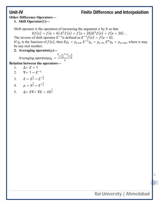
1.1 Finite differences— Let = ( ) be a function and ∆ = ℎ denote the increment in the
independent variable . Assume that∆ , increment in the argument (also known as the
interval or spacing) is fixed. i.e. ℎ =constant . Then the first finite difference y is defined as—
∆ = ∆ ( ) = ( + ∆ ) − ( )
Similarly finite differences of higher orders are denoted as follows—
∆ = ∆(∆ ) = ∆ ( + ∆ ) − ( )
= ∆ ( + ∆ ) − ∆ ( )
= [ ( + 2∆ ) − ( + ∆ )] − [ ( + ∆ ) − ( )]
∆ = ( + 2∆ ) − 2 ( + ∆ ) + ( )
In general ∆ = ∆(∆ ), for = 2,3,4 …
Now consider the function = ( )specified by the tabulated series = ( ) for a set of
equivalent points where = 0,1,2, … , and ∆ = ∆ − = ℎ =constant. Thus the
tabulated function consists of ordered pairs ( , ), ( , ), … , ( , ), …. Here entries
are known as entries.
1.2 Forward Difference—
The first forward difference is denoted by ∆ and defined as
∆ = − .
The symbol ∆ is the forward difference operator.
Properties—
1. ∆ = 0 (Differences of constant function are zero)
2. ∆( ) = ∆( ), where is a constant .
3. ∆( + ) = ∆ + ∆
4. ∆( ) = ∆ + ∆
5. ∆ (∆ ) = ∆
6. Where and are non-negative integers and ∆ = (By definition).
7. The higher order forward difference are defined as:
8. The second order forward difference of is
9. ∆ = ∆(∆ ) = ∆ − ∆
In general,
∆ = ∆(∆ ) = ∆ − ∆
It defines the nth
order forward differences.
Any higher order forward differences can be expressed in terms of the successive values of
the function.
Example:
1.
∆ = − 2 +
2.
∆ = − 3 + 3 −](https://image.slidesharecdn.com/933167d1-d12a-4e85-90a7-e5817f052786-160126124713/85/engineeringmathematics-iv_unit-iv-3-320.jpg)
![Unit-IV Finite Difference and Interpolation
Rai University | Ahmedabad
6
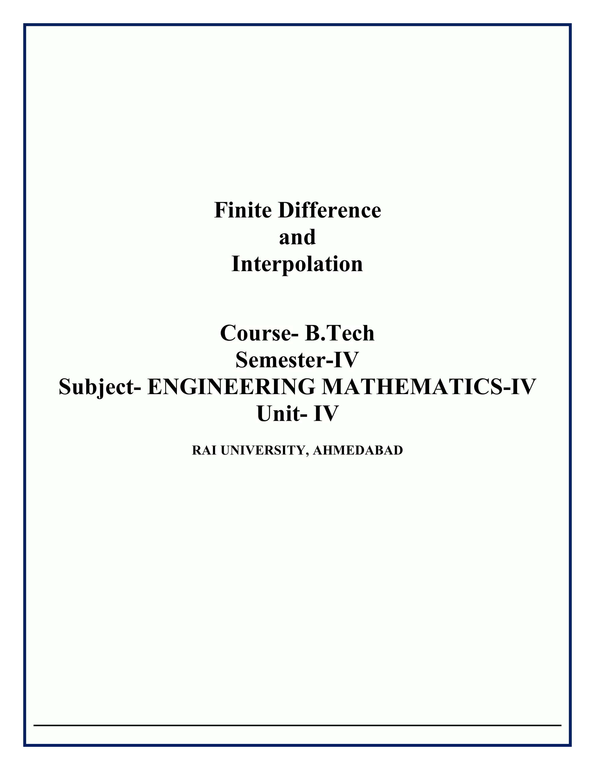
(ii) ∆ log 2 = log 2( + ℎ) − log 2
= log 2( + ℎ) − log 2 + log 2 − log 2
= [log 2( + ℎ) − log 2 ] + [ − ] log 2
= log
+ ℎ
+ [ − 1] log 2
= log 1 +
ℎ
+ ( − 1) log 2
(iii) ∆ = ∆ ( )( )
= ∆ +
= ∆ ∆ + ∆
= ∆ 2 − + 3 −
= 2∆ ( )( )
+3∆ ( )( )
= −2∆ ( )( )
−3∆ ( )( )
= −2 ( )( )
− ( )( )
− 3 ( )( )
− ( )( )
= ( )( )( )
+ ( )( )( )
=
( ) ( )
( )( )( )( )
= ( )( )( )( )
= ( )( )( )( )
=
( )
( )( )( )( )
(iv) ∆ ( ) = − = ( − 1)
∆ ( ) = ∆ (∆ ) = ∆[( − 1) ] = ( − 1)∆ = ( − 1)( − 1)
∆ ( ) = ( − 1)
∆ ( ) = ( − 1)
∆ ( ) = ( − 1)
⋮
∆ ( ) = ( − 1) .
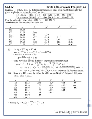
1.5 Difference of a polynomial— The nth
difference of the nth -
degree polynomial are constant
and all higher order differences are zero.
Let the polynomial of nth
degree in is:
( ) = + + … + ( + ℎ) +
∆ ( ) = ( + ℎ) − ( )
= [( + ℎ) − ] + [( + ℎ) − ] + ⋯ + ℎ
= ℎ + + + ⋯ + + ′
Where , , … , ′ are new constants.
Thus the first difference of a polynomial of nth -
degree is a polynomial of degree ( − 1).](https://image.slidesharecdn.com/933167d1-d12a-4e85-90a7-e5817f052786-160126124713/85/engineeringmathematics-iv_unit-iv-6-320.jpg)
![Unit-IV Finite Difference and Interpolation
Rai University | Ahmedabad
7
Similarly
∆ ( ) = ∆[ ( + ℎ) − ( )] = ∆ ( + ℎ) − ∆ ( )
= ℎ[( + ℎ) − ] + [( + ℎ) − ] + ⋯ + ℎ
= ( − 1)ℎ + + + ⋯ + ′′
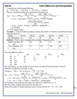
∴ the second differences represent a polynomial of degree ( − 2).
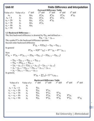
Continuing in this process for the nth differences we get a polynomial of degree zero.
i.e. ∆ ( ) = ( − 1)( − 2) … 1
ℎ = ! ℎ , which is constant.
Hence the ( + 1)th
and higher order differences of a polynomial of nth
degree will be zero.
Example— Evaluate ∆ [(1 − )(1 − )(1 − )(1 − )].
Solution— ∆ [(1 − )(1 − )(1 − )(1 − )]
= ∆ [ + (. . . ) + (… ) + ⋯ + 1]
= (10!) [∵ ∆ ( ) = 0 < 10]
Example— Find the missing value of the following table:
: 45 50 55 60 65
: 3.0 _______ 2.0 ________ -2.4
Solution—The difference is –
∆ ∆ ∆
45 = 3.0 − 3 5 − 2 3 + − 9
50 2 − + − 4 3.6 − − 3
55 = 2.0 − 2 −0.4 − 2
60 −2.4 −
65 = −2.4
Solving the two equations 3 + − 9 = 0 and 3.6 − − 3 = 0.
we can find the value of and .
3 + = 9 … ( )
+ 3 = 3.6 … ( )
From ( )
= 9 − 3 .
Substituting the value of ( )
+ 3(9 − 3 ) = 3.6
⟹ −8 = 3.6 − 27
⟹ =
−23.4
−8
= 2.935
= 9 − 3(2.935) = 9 − 8.775 = 0.225.](https://image.slidesharecdn.com/933167d1-d12a-4e85-90a7-e5817f052786-160126124713/85/engineeringmathematics-iv_unit-iv-7-320.jpg)
![Unit-IV Finite Difference and Interpolation
Rai University | Ahmedabad
9
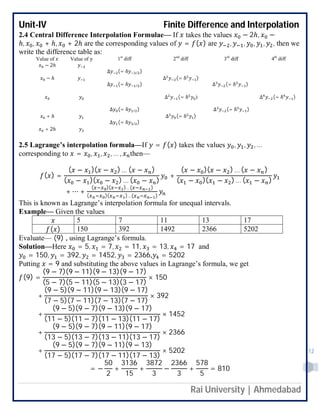
2.1 Interpolation—Let = ( ) is tabulated for the equally spaced values of
= , , , … , , where = + ℎ, = 0,1,2, … ,
⟹ = + ℎ,
= + 2ℎ
= + 3ℎ
= + ℎ
It gives— = , , ,… ,
…
…
The process of finding the values of corresponding to any value of = between and
is called interpolation.
The study of interpolation is based on the concept of difference of a function.
To determine the values of ( ) of ′( ) for some intermediate values of various types of
difference are very much useful.
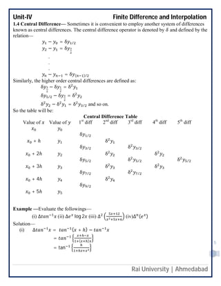
2.2 Newton’s forward difference interpolation— Let the function = ( ) takes the values
, , ,… corresponding to the values , + ℎ, + 2ℎ, … of . Suppose it is required to
evaluate ( ) for = + ℎ, where is any real number.
For any real number , we have defined such that—
( ) = ( + ℎ)
= ( + ℎ) = ( ) = (1 + ∆) [∵ = 1 +△]
= 1 + △ +
( )
!
△ +
( )( )
!
△ + ⋯ [Binomial theorem]
= + △ +
( )
!
△ +
( )( )
!
△ + ⋯ … (1)
It is called Newton’s forward difference interpolation formula as (1) contains and the
forward differences of .
2.3 Newton’s backward difference interpolation— Let the function = ( ) takes the
values , , ,… corresponding to the values , + ℎ, + 2ℎ, … of . Suppose it is
required to evaluate ( ) for
= + ℎ, where is any real number.
Then we have
= ( + ℎ) = ( ) = (1 − ∇) [∵ = 1 − ∇]
= 1 + ∇ +
( )
!
∇ +
( )( )
!
∇ + ⋯ [ ℎ ]
= + ∇ +
( )
!
∇ +
( )( )
!
∇ + ⋯ … (2)
It is called Newton’s forward difference interpolation formula as eq (1) contains and the
forward differences of .](https://image.slidesharecdn.com/933167d1-d12a-4e85-90a7-e5817f052786-160126124713/85/engineeringmathematics-iv_unit-iv-9-320.jpg)
![Unit-IV Finite Difference and Interpolation
Rai University | Ahmedabad
13
2.6 Divided difference—
TheLagrange’s formula has the drawback that if another interpolation areinterested then the
interpolation coefficient are required to recalculate.
This problem is solved in Newton’s divided difference interpolation formula.
If ( , ), ( , ), ( , ) … be given points, then the first divided difference for the argument
is , is defined by the relation [ , ] = .
Similarly,
[ , ] = and[ , ] = etc.
The second divided difference for the argument is , , is defined as [ , , ] =
[ ] [ , ]
.
The third divided difference for the argument is , , , is defined as [ , , , ] =
[ , , ] [ , , ]
and so on.
2.7 Newton’s divided difference interpolation formula— Let , , , … be the values of
= ( ) corresponding to the arguments , , , … , . Then from the definition of divided
differences, we have [ , ] =
= +( − )[ − ] … ( )
Again, [ , , ] =
[ , ] [ , ]
Which give—
[ , ] = [ , ] +( − ) + ( − ) [ , , ]
Substituting this values in the eq(i), we get
= +( − )[ − ] + ( − )( − ) [ , , ] … ( )
Also, [ , , , ] =
[ , , ] [ , , ]
Which gives [ , , ] = [ , , ] −( , )[ , , , ]
Substituting this values of [ , , ] in the eq(ii), we obtain
= +( − )[ − ] + ( − )( − ) [ , , ]
+( − )( − ) ( − )[ , , , ]
Proceeding in this way, we get
= +( − )[ − ] + ( − )( − ) [ , , ]
+( − )( − )( − )[ , , , ] + ⋯
+( − )( − ) … ( − )[ , , , … , ] … ( )
This is called as Newton’s divided difference interpolation formula.](https://image.slidesharecdn.com/933167d1-d12a-4e85-90a7-e5817f052786-160126124713/85/engineeringmathematics-iv_unit-iv-13-320.jpg)
![Unit-IV Finite Difference and Interpolation
Rai University | Ahmedabad
15
Applying Newton’s divided difference formula—
( ) = ( ) + 0 +( − )[ − ] + ( − )( − ) [ , , ] + ⋯
= 1245 + ( + 4)(−404) + ( + 4)( + 1)(94)
+( + 4)( + 1)( − 0)(−14) + ( + 4) ( + 1)( − 2)(3)
= 3 + 5 + 6 − 14 + 5](https://image.slidesharecdn.com/933167d1-d12a-4e85-90a7-e5817f052786-160126124713/85/engineeringmathematics-iv_unit-iv-15-320.jpg)
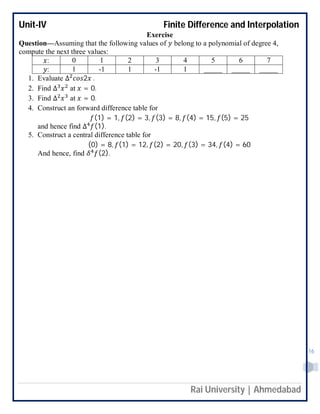


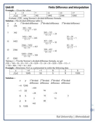
This document discusses finite difference and interpolation methods. It defines finite differences of various orders (first, second, etc.) and describes forward, backward, and central difference tables. It also covers Newton's forward and backward interpolation formulas for unequal intervals using forward and backward differences. An example is provided to illustrate calculating interpolated values using these formulas.