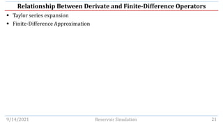
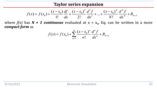
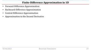
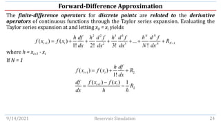
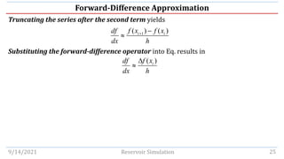
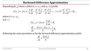
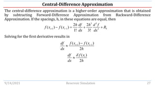
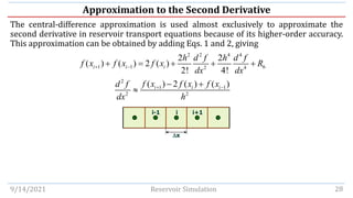
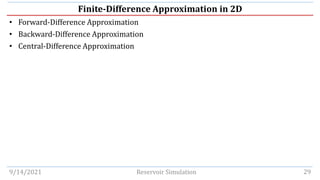
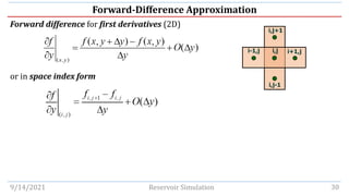
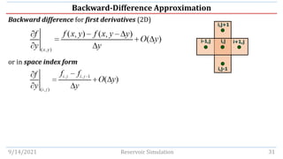
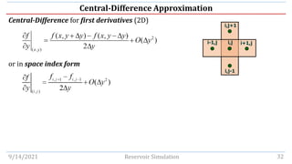
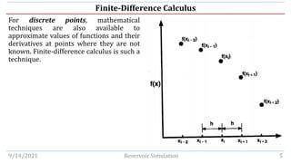
This document discusses finite-difference calculus techniques used to approximate values of functions and derivatives at discrete points in reservoir simulation models. It introduces common finite-difference operators - including forward, backward, central, shift, and average operators - and examines their relationships to derivative operators in Taylor series expansions. Examples are provided to demonstrate calculating finite-difference approximations of first and second derivatives in 1D and 2D. The document also covers solving the Poisson equation and time-independent partial differential equations using finite-difference methods.

1. Vietnam National University - Ho Chi Minh City
University of Technology
Faculty of Geology & Petroleum Engineering
Department of Drilling - Production Engineering
Course
Reservoir Simulation
Trần Nguyễn Thiện Tâm
trantam2512@hcmut.edu.vn

2. Chapter 3
Finite-Difference Calculus
9/14/2021 Reservoir Simulation 2

3. References
Turgay Ertekin, Jamal H. Abou-Kassem, Gregory R. King. Basic Applied Reservoir
Simulation. Society of Petroleum Engineers, 2001.
9/14/2021 Reservoir Simulation 3

4. Contents
❑ Finite-Difference Operators
❑ Relationship Between Derivate and Finite-Difference Operators
9/14/2021 Reservoir Simulation 4

5. Finite-Difference Calculus
For discrete points, mathematical
techniques are also available to
approximate values of functions and their
derivatives at points where they are not
known. Finite-difference calculus is such a
technique.
9/14/2021 Reservoir Simulation 5

6. Finite-Difference Operators
The basis of finite-difference calculus is a group of operators that acts on discrete
points. An operator is a sequence of mathematical operations performed in a fixed
order that acts on any number of the discrete points and results in a final number. The
operators used in finite-difference calculus include:
• the forward-difference operator, Δ;
• the backward-difference operator, 𝛻;
• the central-difference operator, δ;
• the shift (translation) operator, E;
• and the average operator, A.
9/14/2021 Reservoir Simulation 6

7. Finite-Difference Operators
▪ Forward-Difference Operator
▪ Backward-Difference Operator
▪ Central-Difference Operator
▪ Shift (Translation) Operator
▪ Average Operator
9/14/2021 Reservoir Simulation 7

8. Forward-Difference Operator
The forward-difference operator, Δ, operating on a function, f(xi), is defined as
Δf(xi) = f(xi+1) – f(xi)
xi and xi+1 = the discrete points
f(xi) and f(xi+1) = the functional values at these discrete points
9/14/2021 Reservoir Simulation 8

9. Forward-Difference Operator
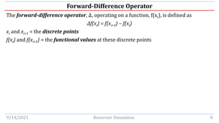
Similarly, the second-order forward-difference operator is defined as
Δ2f(xi) = Δ[Δf(xi)]
= Δ[f(xi+1) – f(xi)]
= Δf(xi+1) - Δf(xi)
= [f(xi+2) – f(xi+1)]- [f(xi+1) – f(xi)]
= f(xi+2) - 2f(xi+1) + f(xi)
9/14/2021 Reservoir Simulation 9

10. Example
With the series of values listed in Table
3.2. Note that the values in this table were
generated by the formulas f(xi) = sin(xi)
and g(xi) = cos(xi).
Calculate the Δf(xi), Δ2g(xi) and Δ[g(xi)f(xi)]
at x = π/4.
9/14/2021 Reservoir Simulation 10

11. Backward-Difference Operator
The backward-difference operator,∇, operating on a function, f(xi), is defined as
∇f(xi) = f(xi) – f(xi-1)
xi and xi-1 = the discrete points
f(xi) and f(xi-1) = the functional values at these discrete points
9/14/2021 Reservoir Simulation 11

12. Backward-Difference Operator
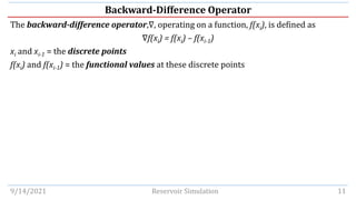
Similarly, the second-order backward-difference operator is defined as
∇2f(xi) = ∇[∇f(xi)]
= ∇[f(xi) – f(xi-1)]
= ∇f(xi) - ∇f(xi-1)
= [f(xi) – f(xi-1)]- [f(xi-1) – f(xi-2)]
= f(xi) - 2f(xi-1) + f(xi-2)
9/14/2021 Reservoir Simulation 12

13. Example
With the series of values listed in Table
3.2. Note that the values in this table were
generated by the formulas f(xi) = sin(xi)
and g(xi) = cos(xi).
Calculate the ∇f(xi), ∇2g(xi) and ∇[g(xi)f(xi)]
at x = π/4.
9/14/2021 Reservoir Simulation 13

14. Central-Difference Operator
The central-difference operator, δ, operating on a function, f(xi), is defined as
δf(xi) = f(xi+1/2) – f(xi-1/2)
An altemative definition of the central-difference operator is
δf(xi) = f(xi+1) – f(xi-1)
9/14/2021 Reservoir Simulation 14

15. Central-Difference Operator
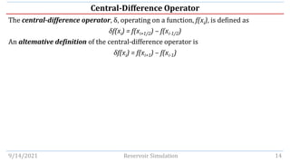
Similarly, the second-order central-difference operator is defined as
δ2f(xi) =δ[δf(xi)]
=δ[f(xi+1/2) – f(xi-1/2)]
= δf(xi+1/2) - δf(xi-1/2)
= [f(xi+1) – f(xi)]- [f(xi) – f(xi-1)]
= f(xi+1) - 2f(xi) + f(xi-1)
9/14/2021 Reservoir Simulation 15

16. Example
With the series of values listed in Table
3.2. Note that the values in this table were
generated by the formulas f(xi) = sin(xi)
and g(xi) = cos(xi).
Calculate the δf(xi), δ2g(xi) and δ[g(xi)f(xi)]
at x = π/4.
9/14/2021 Reservoir Simulation 16

17. Shift (Translation) Operator
The shift (translation) operator, E, operating on f(xi) is defined as
Ef(xi) = f(xi+1)
Similarly, the inverse of the shift operator, E-1, operating on f(xi) is defined as
E-1f(xi) = f(xi-1)
In general, the kth-order shift operator is defined by
Ekf(xi) = f(xi+k)
and the kth inverse of the shift operator is defined as
E-k f(xi) = f(xi-k)
9/14/2021 Reservoir Simulation 17

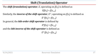
18. Example
With the series of values listed in Table
3.2. Note that the values in this table were
generated by the formulas f(xi) = sin(xi)
and g(xi) = cos(xi).
Calculate the Ef(xi), E2g(xi) and E[g(xi)f(xi)]
at x = π/4.
9/14/2021 Reservoir Simulation 18

19. Average Operator
The average operator, A, operating on f(xi) is defined as
9/14/2021 Reservoir Simulation 19
1/2 1/2
( ) ( )
[ ( )]
2
i i
i
f x f x
A f x + −
+
=

20. Example
With the series of values listed in Table
3.2. Note that the values in this table were
generated by the formulas f(xi) = sin(xi)
and g(xi) = cos(xi).
Calculate the Af(xi), A2g(xi) and A[g(xi)f(xi)]
at x = π/4.
9/14/2021 Reservoir Simulation 20

21. Relationship Between Derivate and Finite-Difference Operators
▪ Taylor series expansion
▪ Finite-Difference Approximation
9/14/2021 Reservoir Simulation 21

22. Taylor series expansion
where f(x) has N + 1 continuous evaluated at x = x0. Eq. can be written in a more
compact form as
9/14/2021 Reservoir Simulation 22
2 2
0 0 0
0 1
2
( ) ( ) ( )
( ) ( ) ...
1! 2! !
N N
N
N
x x x x x x
df d f d f
f x f x R
dx dx N dx
+
− − −
= + + + + +
0
0 1
1
( )
( ) ( )
!
n n
N
N
n
n
x x d f
f x f x R
n dx
+
=
−
= + +


23. Finite-Difference Approximation in 1D
• Forward-Difference Approximation
• Backward-Difference Approximation
• Central-Difference Approximation
• Approximation to the Second Derivative
9/14/2021 Reservoir Simulation 23

24. Forward-Difference Approximation
The finite-difference operators for discrete points are related to the derivative
operators of continuous functions through the Taylor series expansion. Evaluating the
Taylor series expansion at and letting x0 = xi yields
where h = xi+1 - xi
If N = 1
9/14/2021 Reservoir Simulation 24
2 2 3 3
1 1
2 3
( ) ( ) ...
1! 2! 3! !
N N
i i N
N
h df h d f h d f h d f
f x f x R
dx dx dx N dx
+ +
= + + + + + +
1 2
( ) ( )
1!
i i
h df
f x f x R
dx
+ = + +
1
2
( ) ( ) 1
i i
f x f x
df
R
dx h h
+ −
= −

25. Forward-Difference Approximation
Truncating the series after the second term yields
Substituting the forward-difference operator into Eq. results in
9/14/2021 Reservoir Simulation 25
1
( ) ( )
i i
f x f x
df
dx h
+ −

( )
i
f x
df
dx h



26. Backward-Difference Approximation
Expanding f(xi-1) about xi (that is, x = xi-1 and x0 = xi) yields
where h = xi – xi-1
If N = 1
Following the same procedure as for the forward-difference approximation yields
9/14/2021 Reservoir Simulation 26
2 2 3 3
1 1
2 3
( ) ( ) ... ( 1)
1! 2! 3! !
N N
N
i i N
N
h df h d f h d f h d f
f x f x R
dx dx dx N dx
− +
= − + − + + − +
1 2
( ) ( )
1!
i i
h df
f x f x R
dx
− = − +
1
2
( ) ( ) 1
i i
f x f x
df
R
dx h h
−
−
= +
( )
i
f x
df
dx h



27. Central-Difference Approximation
The central-difference approximation is a higher-order approximation that is obtained
by subtracting Forward-Difference Approximation from Backward-Difference
Approximation. If the spacings, h, in these equations are equal, then
Solving for the first derivative results in
9/14/2021 Reservoir Simulation 27
3 3
1 1 5
3
2 2
( ) ( )
1! 3!
i i
h df h d f
f x f x R
dx dx
+ −
− = + +
1 1
( ) ( )
2
i i
f x f x
df
dx h
+ −
−

( )
2
i
f x
df
dx h



28. Approximation to the Second Derivative
The central-difference approximation is used almost exclusively to approximate the
second derivative in reservoir transport equations because of its higher-order accuracy.
This approximation can be obtained by adding Eqs. 1 and 2, giving
9/14/2021 Reservoir Simulation 28
2 2 4 4
1 1 6
2 4
2 2
( ) ( ) 2 ( )
2! 4!
i i i
h d f h d f
f x f x f x R
dx dx
+ −
+ = + + +
2
1 1
2 2
( ) 2 ( ) ( )
i i i
f x f x f x
d f
dx h
+ −
− +

i-1 i i+1
x

29. Finite-Difference Approximation in 2D
• Forward-Difference Approximation
• Backward-Difference Approximation
• Central-Difference Approximation
9/14/2021 Reservoir Simulation 29

30. Forward-Difference Approximation
Forward difference for first derivatives (2D)
or in space index form
9/14/2021 Reservoir Simulation 30
i-1,j i,j i+1,j
i,j+1
i,j-1

31. Backward-Difference Approximation
Backward difference for first derivatives (2D)
or in space index form
9/14/2021 Reservoir Simulation 31
i-1,j i,j i+1,j
i,j+1
i,j-1

32. Central-Difference Approximation
Central-Difference for first derivatives (2D)
or in space index form
9/14/2021 Reservoir Simulation 32
i-1,j i,j i+1,j
i,j+1
i,j-1

33. Central-Difference Approximation
Centered difference for second derivatives (2D)
or in space index form
9/14/2021 Reservoir Simulation 33
i-1,j i,j i+1,j
i,j+1
i,j-1
2
2
2 2
( , )
( , ) 2 ( , ) ( , )
( )
x y
f f x y y f x y f x y y
O y
y y
 +  − + − 
= + 
 
2
, 1 , , 1 2
2 2
( , )
2
( )
i j i j i j
i j
f f f
f
O y
y y
+ −
− +

= + 
 

34. Solving time-independent PDEs
Solve the following Poisson equation:
subject to the boundary conditions:
p = 2 at x = 0 and x = 1
9/14/2021 Reservoir Simulation 34

35. Solving time-independent PDEs
Solve the following Poisson equation:
subject to the boundary conditions:
u = 0 along the boundaries x = 0, x = 1, y = 0, y = 1
9/14/2021 Reservoir Simulation 35