The document provides notes on signals and systems from an EECE 301 course. It includes: - An overview of continuous-time (C-T) and discrete-time (D-T) signal and system models. - Details on chapters covering differentials/differences, convolution, Fourier analysis (both C-T and D-T), Laplace transforms, and Z-transforms. - Examples of calculating the Fourier transform of specific signals like a decaying exponential and rectangular pulse. These illustrate properties of the Fourier transform.

1. 1/27
EECE 301
Signals & Systems
Prof. Mark Fowler
Note Set #14
• C-T Signals: Fourier Transform (for Non-Periodic Signals)
• Reading Assignment: Section 3.4 & 3.5 of Kamen and Heck

2. 2/27
Ch. 1 Intro
C-T Signal Model
Functions on Real Line
D-T Signal Model
Functions on Integers
System Properties
LTI
Causal
Etc
Ch. 2 Diff Eqs
C-T System Model
Differential Equations
D-T Signal Model
Difference Equations
Zero-State Response
Zero-Input Response
Characteristic Eq.
Ch. 2 Convolution
C-T System Model
Convolution Integral
D-T System Model
Convolution Sum
Ch. 3: CT Fourier
Signal Models
Fourier Series
Periodic Signals
Fourier Transform (CTFT)
Non-Periodic Signals
New System Model
New Signal
Models
Ch. 5: CT Fourier
System Models
Frequency Response
Based on Fourier Transform
New System Model
Ch. 4: DT Fourier
Signal Models
DTFT
(for “Hand” Analysis)
DFT & FFT
(for Computer Analysis)
New Signal
Model
Powerful
Analysis Tool
Ch. 6 & 8: Laplace
Models for CT
Signals & Systems
Transfer Function
New System Model
Ch. 7: Z Trans.
Models for DT
Signals & Systems
Transfer Function
New System
Model
Ch. 5: DT Fourier
System Models
Freq. Response for DT
Based on DTFT
New System Model
Course Flow Diagram
The arrows here show conceptual flow between ideas. Note the parallel structure between
the pink blocks (C-T Freq. Analysis) and the blue blocks (D-T Freq. Analysis).

3. 3/27
4.3 Fourier Transform
Recall: Fourier Series represents a periodic signal as a sum of sinusoids
Note: Because the FS uses “harmonically related” frequencies kω0, it can only create
periodic signals
∑
∞
−∞=
=
k
tj
k
k
ectx ω
)(
or complex sinusoids
tjk
e 0ω
With arbitrary discrete frequencies…
NOT harmonically related
∑
∞
−∞=
=
k
tj
k
k
ectx ω
)(The problem with is that it cannot include all possible
frequencies!
Q: Can we modify the FS idea to handle non-periodic signals?
A: Yes!!
What about ?
That will give some non-periodic signals but not some that are
important!!

4. 4/27
How about:
∫
∞
∞−
= ωω
π
ω
deXtx tj
)(
2
1
)(
Called the “Fourier
Integral” also, more
commonly, called the
“Inverse Fourier
Transform”
Plays the
role of ck
Plays the role of
tjk
e 0ω
Integral replaces sum because it can “add up
over the continuum of frequencies”!
Okay… given x(t) how do we get X(ω)?
∫
∞
∞−
−
= dtetxX tjω
ω )()(
Note: X(ω) is complex-valued function of ω ∈ (-∞, ∞)
|X(ω)| )(ωX∠
Yes… this will work for any
practical non-periodic signal!!
Called the
“Fourier Transform”
of x(t)
Need to use two
plots to show it

5. 5/27
Comparison of FT and FS
Fourier Series: Used for periodic signals
Fourier Transform: Used for non-periodic signals (although we
will see later that it can also be used for periodic signals)
∑
∞
−∞=
=
n
tjk
kectx 0
)( ω
∫
+
−
=
Tt
t
tjk
k dtetx
T
c
0
0
0
)(
1 ω
∫
∞
∞−
= ωω
π
ω
deXtx tj
)(
2
1
)( ∫
∞
∞−
−
= dtetxX tjω
ω )()(
Synthesis Analysis
Fourier
Series
Fourier Series Fourier Coefficients
Fourier
Transform
Inverse Fourier Transform Fourier Transform
FS coefficients ck are a complex-valued function of integer k
FT X(ω) is a complex-valued function of the variable ω ∈ (-∞, ∞)

6. 6/27
Synthesis Viewpoints:
We need two plots to show these
∑
∞
−∞=
=
n
tjk
kectx 0
)( ω
|X(ω)| shows how much there is in the signal at frequency ω
∠ X(ω) shows how much phase shift is needed at frequency ω
∫
∞
∞−
= ωω
π
ω
deXtx tj
)(
2
1
)(
We need two plots to show these
FS:
|ck| shows how much there is of the signal at frequency kω0
∠ck shows how much phase shift is needed at frequency kω0
FT:

7. 7/27
Some FT Notation:
)()( ωXtx ↔1.
If X(ω) is the Fourier transform of x(t)…
then we can write this in several ways:
{ })()( txX F=ω2. ⇒ F{ } is an “operator” that operates on x(t) to give X(ω)
⇒ F-1{ } is an “operator” that operates on X(ω) to give x(t){ })()( 1
ωXtx −
= F3.

8. 8/27
Analogy: Looking at X(ω) is “like” looking at an x-ray of the signal- in the sense that an
x-ray lets you see what is inside the object… shows what stuff it is made from.
In this sense: X(ω) shows what is “inside” the signal – it shows how much of each complex
sinusoid is “inside” the signal
Note: x(t) completely determines X(ω)
X(ω) completely determines x(t)
There are some advanced mathematical issues
that can be hurled at these comments… we’ll
not worry about them

9. 9/27
FT Example: Decaying Exponential
Given a signal x(t) = e-btu(t) find X(ω) if b > 0
Now…apply the definition of the Fourier transform. Recall the general
form:
dtetxX tj
∫
∞
∞−
−
= ω
ω )()(
1
)(tx
t
b controls decay rate
The u(t) part forces this to zero
What does this look
like if b < 0???
Solution: First see what x(t) looks like:

10. 10/27
dtetueX tjbt
∫
∞
∞−
−−
= ω
ω )()(
Easy
integral!
[ ]0)()(
0
)( 11 ωωω
ωω
jbjb
t
t
tjb
ee
jb
e
jb
+−∞+−
∞=
=
+−
−
+
−
=⎥
⎦
⎤
⎢
⎣
⎡
+
−
=
[ ]10
1
−
+
−
=
ωjb
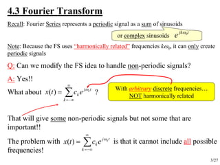
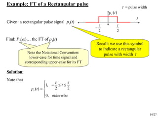
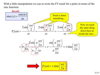
Now plug in for our signal:
integrand = 0 for t < 0
due to the u(t)
dtedtee tjbtjbt
∫∫
∞
+−
∞
−−
==
0
)(
0
ωω
Set lower limit to 0
and then u(t) = 1 over
integration range
ωjb +
=
1
⎥
⎥
⎦
⎤
⎢
⎢
⎣
⎡
−
+
−
=
==
∞−
=
∞−
1
0
10
1
eee
jb mag
jb ω
ω
Only if b>0… what
happens if b<0

11. 11/27
ω
ω
jb
X
+
=
1
)(
22
1
)(
ω
ω
+
=
b
X
⎟
⎠
⎞
⎜
⎝
⎛
−=∠ −
b
X
ω
ω 1
tan)(
(Complex Valued)
Magnitude
Phase
)()( tuetx bt−
=
For b > 0
1
)()( tuetx bt−
=
t
b > 0 controls
decay rate
)(ωX
ω
Summary of FT Result for Decaying Exponential

12. 12/27
MATLAB Commands to Compute FT
w=-100:0.2:100;
b=10;
X=1./(b+j*w);
Plotting Commands
subplot(2,1,1); plot(w,abs(X))
xlabel('Frequency omega (rad/sec)')
ylabel('|X(omega|) (volts)'); grid
subplot(2,1,2); plot(w,angle(X))
xlabel('Frequency omega (rad/sec)')
ylabel('<X(omega) (rad)'); grid
Fourier Transform of e-btu(t) for b = 10
Note that
magnitude
plot has even
symmetry
Note that
phase plot has
odd symmetry
True for every
real-valued signal
Note: Book’s Fig. 3.12 only
shows one-sided spectrum plots
(volts)
Technically V/Hz

13. 13/27
-10 0 10 20 30 40
0
0.5
1
t (sec)
x(t)
-100 -50 0 50 100
0
5
10
ω (rad/sec)
|X(ω)|
-10 0 10 20 30 40
0
0.5
1
t (sec)
x(t)
-100 -50 0 50 100
0
0.5
1
ω (rad/sec)
|X(ω)|
-10 0 10 20 30 40
0
0.5
1
t (sec)
x(t)
-100 -50 0 50 100
0
0.05
0.1
ω (rad/sec)
|X(ω)|
b=0.1 b=0.1
b=1 b=1
b=10 b=10
Note: As b increases…
1. Decay rate in time signal increases
2. High frequencies in Fourier transform are more prominent.
Time Signal Fourier Transform
Exploring
Effect of
decay rate b
on the
Fourier
Transform’s
Shape
Short Signals have FTs that spread
more into High Frequencies!!!

14. 14/27
Example: FT of a Rectangular pulse
Given: a rectangular pulse signal pτ(t)
t
2
τ
2
τ
−
)(tpτ
τ = pulse width
Recall: we use this symbol
to indicate a rectangular
pulse with width τ
⎪
⎩
⎪
⎨
⎧
≤≤−
=
otherwise
t
tp
,0
22
,1
)(
ττ
τ
Solution:
Note that
Note the Notational Convention:
lower-case for time signal and
corresponding upper-case for its FT
Note the Notational Convention:
lower-case for time signal and
corresponding upper-case for its FT
Find: Pτ(ω)… the FT of pτ(t)

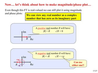
15. 15/27
∫∫ −
−
∞
∞−
−
==
2/
2/
)()(
τ
τ
ωω
ττ ω dtedtetpP tjtj
[ ]
⎥
⎥
⎥
⎦
⎤
⎢
⎢
⎢
⎣
⎡
−
=
−
=
−
−
−
2
21 22
2
2 j
ee
e
j
jj
tj
ωτωτ
τ
τ
ω
ωω
Artificially
inserted 2 in
numerator and
denominator
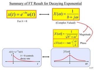
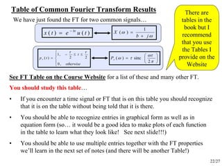
Now apply the definition of the FT: Limit integral to
where pτ(t) is non-
zero… and use the
fact that it is 1 over
that region
⎟
⎠
⎞
⎜
⎝
⎛
=
2
sin
ωτ Use Euler’s
Formula
ω
ωτ
ωτ
⎟
⎠
⎞
⎜
⎝
⎛
=
2
sin2
)(P
sin goes up and down
between -1 and 1
1/ω decays down as |ω| gets
big… this causes the overall
function to decay down

16. 16/27
For this case the FT is real valued so we can plot it using a single plot
(shown in solid blue here):
2/ω
2/ω
-2/ω
-2/ω
ω
ωτ
ωτ
⎟
⎠
⎞
⎜
⎝
⎛
=
2
sin2
)(P
The sin wiggles up down
“between ±2/ω”
The sine wiggles up &
down “between ±2/ω”
τ = 1/2

17. 17/27
Even though this FT is real-valued we can still plot it using magnitude
and phase plots:
We can view any real number as a complex
number that has zero as its imaginary part
Re
Im
A positive real number R will have:
|R| = R ∠R = 0
R
Re
Im
A negative real number R will have:
|R| = -R ∠R = ±π
R
+π
-π
Can use
either one!!
Now… let’s think about how to make magnitude/phase plot…

18. 18/27
Applying these Ideas to the Real-valued FT Pτ(ω)
Phase = 0
Phase = ±π
Here I have chosen -π to display odd symmetry

19. 19/27
-4 -3 -2 -1 0 1 2 3 4
0
0.5
1
t (sec)
x(t)
-100 -50 0 50 100
0
1
2
ω (rad/sec)
|X(ω)|
-4 -3 -2 -1 0 1 2 3 4
0
0.5
1
t (sec)
x(t)
-100 -50 0 50 100
0
0.5
1
ω (rad/sec)
|X(ω)|
-4 -3 -2 -1 0 1 2 3 4
0
0.5
1
t (sec)
x(t)
-100 -50 0 50 100
0
0.5
1
ω (rad/sec)
|X(ω)|
τ = 2 τ = 2
τ = 1 τ = 1
τ = 1/2 τ = 1/2
Note: As width decreases, FT is more widely spread
Narrow pulses “take up more frequency range”
Effect of Pulse Width on the FT Pτ(ω)

20. 20/27
The result we just found had this mathematical form:
ω
ωτ
ωτ
⎟
⎠
⎞
⎜
⎝
⎛
=
2
sin2
)(P
x
x
x
π
π )sin(
)(sinc =
This kind of structure shows up frequently enough
that we define a special function to capture it:
Define:
Note that sinc(0) = 0/0.
So… Why is sinc(0) = 1?
It follows from
L’Hopital’s Rule
Plot of sinc(x)
Definition of “Sinc” Function

21. 21/27
With a little manipulation we can re-write the FT result for a pulse in terms of the
sinc function:
Now we need
the same thing
down here as
inside the sine…
⎟
⎠
⎞
⎜
⎝
⎛
=
π
ωτ
τωτ
2
sinc)(P
Need π times
something…
Need π times
something…
Need π times
something…
⎟
⎠
⎞
⎜
⎝
⎛
=
⎟
⎠
⎞
⎜
⎝
⎛
=
⎟
⎠
⎞
⎜
⎝
⎛
=
π
ωτ
τ
π
ωτ
π
π
ωτ
π
τ
ω
π
τ
π
π
ωτ
π
π
τ
π
2
sinc
2
2
sin
2
2
sin2
2
ω
π
ωτ
π
ω
ωτ
π
π
ω
ωτ
ωτ
⎟
⎠
⎞
⎜
⎝
⎛
=
⎟
⎠
⎞
⎜
⎝
⎛
=
⎟
⎠
⎞
⎜
⎝
⎛
=
2
sin2
2
sin2
2
sin2
)(P
x
x
x
π
π )sin(
)(sinc =
Recall:

22. 22/27
Table of Common Fourier Transform Results
We have just found the FT for two common signals…
ω
ω
jb
X
+
=
1
)()()( tuetx bt−
=
⎪
⎩
⎪
⎨
⎧
≤≤−
=
otherwise
t
tp
,0
22
,1
)(
ττ
τ ⎟
⎠
⎞
⎜
⎝
⎛
=
π
ωτ
τωτ
2
sinc)(P
See FT Table on the Course Website for a list of these and many other FT.
There are
tables in the
book but I
recommend
that you use
the Tables I
provide on the
Website
You should study this table…
• If you encounter a time signal or FT that is on this table you should recognize
that it is on the table without being told that it is there.
• You should be able to recognize entries in graphical form as well as in
equation form (so… it would be a good idea to make plots of each function
in the table to learn what they look like! See next slide!!!)
• You should be able to use multiple entries together with the FT properties
we’ll learn in the next set of notes (and there will be another Table!)

23. 23/27
For your FT Table you should spend time making sketches of the entries
… like this:
t
)(ωX
ω
t
2
τ
2
τ
−
)(tpτ
)(ωτP
ω

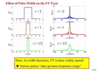
24. 24/27
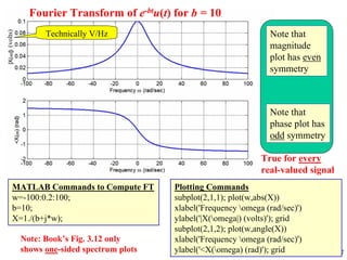
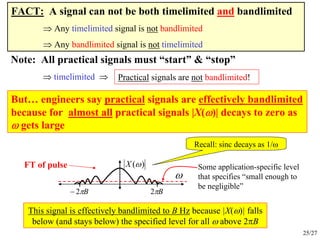
Bandlimited and Timelimited Signals
t
],[0)( 21 TTttx ∉∀=
1T 2T
A signal x(t) is timelimited (or of finite duration) if there are 2 numbers T1 & T2
such that:
A (real-valued) signal x(t) is bandlimited
Now that we have the FT as a tool to analyze signals, we can use it to identify
certain characteristics that many practical signals have.
if there is a number B such that
ωBπ2−
)(ωX
Bπ2
BX πωω 20)( >∀=
2πB is in rad/sec
B is in Hz
Recall: If x(t) is real-valued then |X(ω)| has “even symmetry”

25. 25/27
FACT: A signal can not be both timelimited and bandlimited
⇒ Any timelimited signal is not bandlimited
⇒ Any bandlimited signal is not timelimited
This signal is effectively bandlimited to B Hz because |X(ω)| falls
below (and stays below) the specified level for all ω above 2πB
But… engineers say practical signals are effectively bandlimited
because for almost all practical signals |X(ω)| decays to zero as
ω gets large
Practical signals are not bandlimited!
Note: All practical signals must “start” & “stop”
⇒ timelimited ⇒
ω
Bπ2−
)(ωX
Bπ2
FT of pulse Some application-specific level
that specifies “small enough to
be negligible”
Recall: sinc decays as 1/ω

26. 26/27
Bandwidth (Effective Bandwidth) Abbreviate Bandwidth as “BW”
For a lot of signals – like audio – they fill up the lower frequencies but then decay
as ω gets large:
ω
Bπ2−
)(ωX
Bπ2
We say the signal’s BW = B in Hz if there is “negligible” content for |ω| > 2πB
Must specify what
“negligible” means
For Example:
1. High-Fidelity Audio signals have an accepted BW of about 20 kHz
2. A speech signal on a phone line has a BW of about 4 kHz
Signals like this are
called “lowpass” signals
Early telephone engineers determined that limiting speech to a BW
of 4kHz still allowed listeners to understand the speech

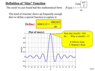
27. 27/27
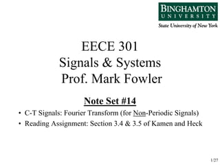
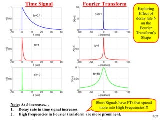
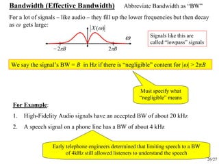
For other kinds of signals – like “radio frequency (RF)” signals – they
are concentrated at high frequencies
ω
)(ωX
1ω−2ω− 11 2 fπω = 22 2 fπω =
If the signal’s FT has negligible content for |ω| ∉ [ω1, ω2]
then we say the signals BW = f2 - f1 in Hz
For Example:
1. The signal transmitted by an FM station has a BW of 200 kHz = 0.2 MHz
a. The station at 90.5 MHz on the “FM Dial” must ensure that its signal
does not extend outside the range [90.4, 90.6] MHz
b. Note that: FM stations all have an odd digit after the decimal point.
This ensures that adjacent bands don’t overlap:
i. FM90.5 covers [90.4, 90.6]
ii. FM90.7 covers [90.6, 90.8], etc.
2. The signal transmitted by an AM station has a BW of 20 kHz
a. A station at 1640 kHz must keep its signal in [1630, 1650] kHz
b. AM stations have an even digit in the tens place and a zero in the ones
Signals like this are
called “bandpass” signals