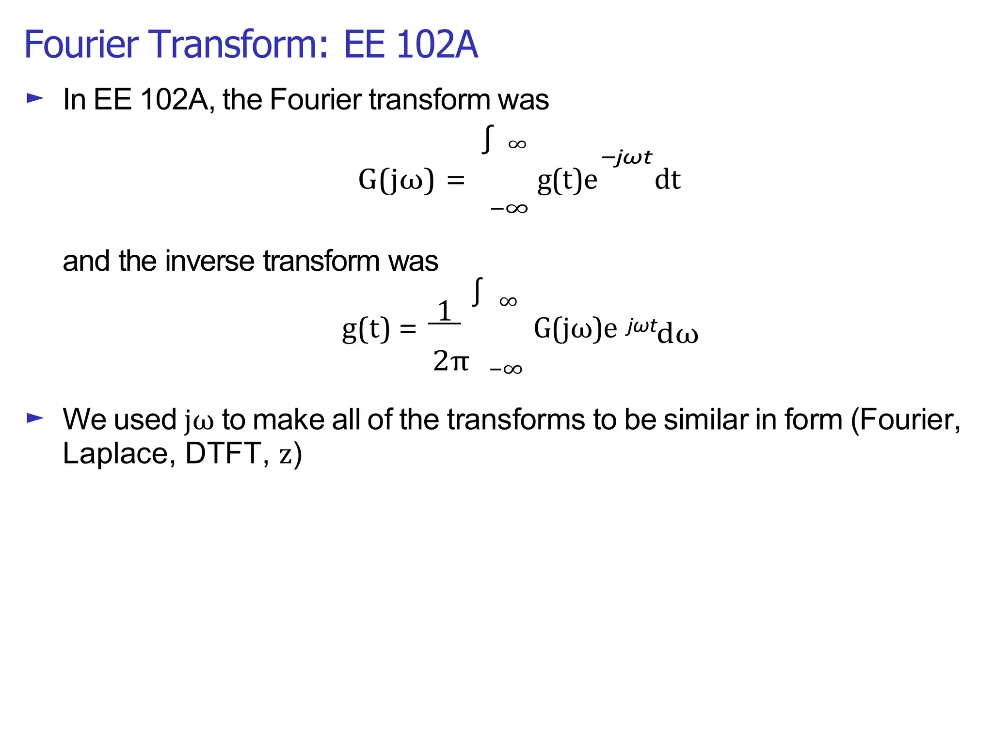
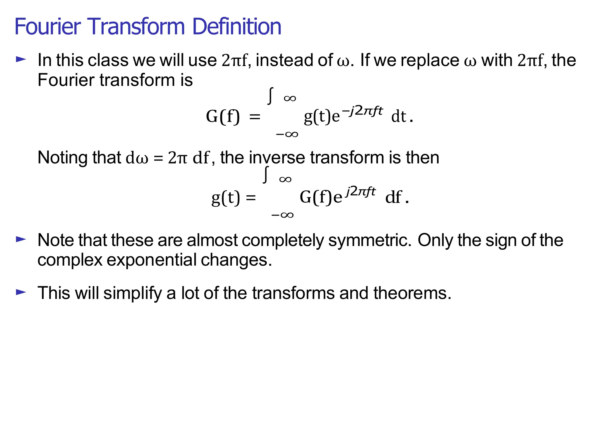
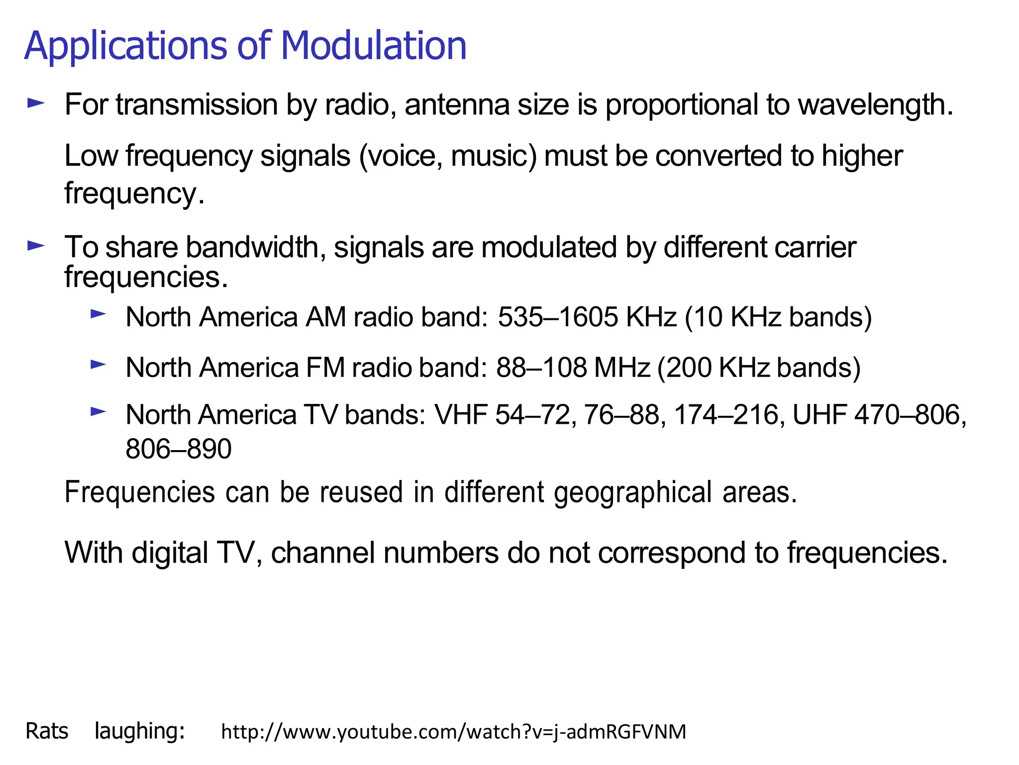
Lecture 4: Review of Signals and Systems,
Frequency Domain
Signals and Systems: Frequency
Today:
► The Fourier transform in 2πf
► Some important Fourier transforms
► Some important Fourier transform theorems
► Hilbert transform and analytic signals
Next Time:
► Communication channels and equalization
► Amplitude modulation
► Modulators
Based on Notes from John Gill
Fourier Transform: EE 102A
► In EE 102A, the Fourier transform was
∫ ∞
−jωt
G(jω) =
and the inverse transform was
g(t)e dt
−∞
g(t) =
1
∫ ∞
G(jω)e jωt
dω
2π −∞
► We used jω to make all of the transforms to be similar in form (Fourier,
Laplace, DTFT, z)
Fourier Transform Definition
∫
► In this class we will use 2πf, instead of ω. If we replace ω with 2πf, the
Fourier transform is
G(f) =
∞
g(t)e
−∞
−j2πft
dt .
Noting that dω = 2π df, the inverse transform is then
g(t) =
∞
G(f)e
−∞
j2πft
df .
► Note that these are almost completely symmetric. Only the sign of the
complex exponential changes.
► This will simplify a lot of the transforms and theorems.
∫
Fourier Transform Existence
| |
−∞
|g(t)| dt < ∞
If g(t) is absolutely integrable, i.e.,
∫ ∞
then G(f) exists for every frequency f and is continuous.
If g(t) has finite energy, i.e.,
∞
g(t) 2
−∞
dt < ∞
then G(f) exists for “most” frequencies f and has finite energy.
If g(t) is periodic and has a Fourier series, then
∞
G(f) =
n=
Σ
−∞
G(nf0)δ(f − nf0)
is a weighted sum of impulses in frequency domain.
∫
Fourier Transform Example in 2πf
(
One-sided exponential decay is defined by e−at
u(t) with a > 0:
g(t) =
0 t < 0
e−at
t > 0
The Fourier transform of one-sided decay is (simple calculus):
G(f) =
∞
e−j2πft
0
e−at
dt =
∞
e−(a+j2πf )t
dt
0
e−(a+j2πf )t
=
−(a + j2πf)
t=∞
=
t=0
1
a + j2πf
Compare this to the EE 102A transform
1
G(jω) =
a + jω
Often you can easily just substitute 2πf for ω.
∫ ∫
Fourier Transform Examples: Real Valued Signals
∫
∫
Many of the signals we will be dealing with are real, such as sound and
video.
In this case the Fourier transform is conjugate symmetric
G∗(f) =
∞
g(t)e
−∞
−j2πft
dt
∗
=
∞
g(t)∗(e
−∞
−j2πft
)∗
dt
∞
= g(t)e
−∞
j2πft
dt =
∞
g(t)e
−∞
−j2π(−f )t
dt = G(−f)
This means that the real part of the signal is even and the imaginary part is
odd. This is called Hermitian symmetry.
This is important because we need only positive frequencies for real-valued
signals.
We will exploit this often!
∫
∫
Duality
−∞
∫
∫
g(t) =
Fourier inversion theorem: if g(t) has a Fourier transform G(f),
∞
G(f) =
∫ ∞
g(t)e−j2πft
dt
j2πft
The inverse transform differs from the forward transform only in the sign of
the exponent.
If we consider G(f) to be a function of t instead of f, and apply the
Fourier Transform again
∞
G(t)e
−∞
−j2πft
dt =
∞
G(t)e
−∞
j2π(−f )t
dt = g(−f)
We can summarize this as
F{g(t)} = G(f) ⇒ F{G(t)} = g(−f)
This is the principle of duality. This is much easier to use with 2πf.
−∞
∫
G(f)e df
Important Fourier Transforms
2
∫
(
1 |t| < 1
The unit rectangle function Π(t) is defined by
Its Fourier transform is
Π(t) = 2
0 |t| > 1
F {Π(t)} =
∞
e−i2πft
−∞
Π(t) dt =
1/2
−1/2
e−i2πft
dt =
sin πf
= sinc(πf)
πf
Π(t) sinc(πf)
Fact: every finite width pulse has a transform with unbounded frequencies.
∫
By duality, we can also find
sinc(πt) Π(f)
since Π(f) is even, so Π(f) = Π(−f).
2 1 0 2 t 1 0 f
Fourier Transform Time Scaling
∫ ∫
|a| a
a
If a > 0 and g(t) is a signal with Fourier transform G(f), then
F {g(at)} =
∞
g(at)e
−∞
−j2πft
dt =
∞
g(u)e
−∞
−j2πfu/a
1
(du/a) = G
a
f
If a < 0, change of variables requires reversing limits of integration:
F {g(at)} = −
1
G
f
a a
Combining both cases:
F {g(at)} =
1
G
f
Special case: a = −1. The Fourier transform of g(−t) is G(−f).
Compressing in time corresponds to expansion in frequency (and reduction
in amplitude) and vice versa.
The sharper the pulse the wider the spectrum.
Fourier Transform Time Scaling Example
F
n ,
∫
The transform of a narrow rectangular pulse of area 1 is
1
Π(t/τ) = sinc(πτf)
τ
In the limit, the pulse is the unit impulse, and its tranform is the constant 1.
We can find the Fourier transform directly:
F{δ(t)} =
so
∞
δ(t)e
−∞
−j2πft
dt = e−j2πft
= 1
t=0
δ(t) 1
The impulse is the mathematical abstraction of signal whose Fourier
transform has magnitude 1 and phase 0 for all frequencies.
By duality, F{1} = δ(f). All DC, no oscillation.
1 δ(f)
Important Fourier Transforms (cont.)
∫
2 2 2
2i 2i 2i
—
► Shifted impulse δ(t − t0):
F{δ(t − t0)} =
∞
δ(t t0)e
−∞
−j2πft
dt = e−j2πft0
This is a complex exponential in frequency.
δ(t − t0) e−j2πft0
Then by duality
► Sinuoids:
ej2πf0t
δ(f − f0)
F{cos 2πf0t} = F{ 1
(ej2πf0t
+ e−j2πf0t
)} = 1
δ(f − f0) + 1
δ(f + f0)
F{sin 2πf0t} = F{ 1
(ej2πf0t
+ e−j2πf0t
)} = 1
δ(f − f0) − 1
δ(f + f0)
Important Fourier Transforms (cont.)
sgn(t) lim e u(t) − e u(−t)
sgn(t)
2 t
► Laplacian pulse g(t) = e−a|t| where a > 0. Since
g(t) = e−at
u(t) + eat
u(−t) ,
we can use reversal and additivity:
1 1 2a
G(f) =
a + j2πf
+
a − j2πf
=
a2 + 4π2f2
.
This is twice the real part of the Fourier transform of e−at
u(t)
► The signum function can be approximated as
► This has the Fourier transform
F {sgn(t)} = lim
1
−
1
=
► The unit step function is
a→0
1
jπf
1
a + j2πf
1
a − j2πf
u(t) =
This has the Fourier transform
+ sgn(t)
2 2
1 1
F{u(t)} = 2 δ(f) +
j2πf
Hilbert Transform
An import filter has an impulse response
1
h(t) =
πt
By duality, using the sgn(t) transform we found above,
H(f) = −j sgn(f)
which looks like this
To see why this is important, consider
1
What does this do?
cos(2πf0t) ∗
πt
Hilbert Transform
Transform
Signal
cos(2⇡f0t)
1
⇡t
sin(2⇡f0t)
It has turned a cosine into a sine! This will turn up frequently.
1
0
f
0
f
0
f
2 πt
Analytic Signal
The dual of the unit step is also useful
1
H(f) = (1 + sgn(f))
2
By duality this corresponds to the impulse response
h(t) =
1
δ(t) +
j
Consider what happens when we take a real signal, and convolve it with h(t)
x(t) ∗ h(t)
What does this do?
Analytic Signal
Transform
Signal
✓
x(t)
1 j
δ(t) +
2 πt 0 f
xa(t)
This is a signal that just has positive frequencies!
We will see this when we talk about signal sideband transmission.
Fourier Transform Properties
∫
2 2
—
► Time delay causes linear phase shift.
F {g(t − t0)} =
∞
g(t t0)e
−∞
−j2πft
dt =
∞
g(u)e
−∞
−j2πf (u+t0)
du
So,
= e−j2πft0
∞
g(u)e
−∞
−j2πfu
du = e−j2πft 0
G(f)
g(t − t0) e−j2πft0
G(f)
► Then, by duality, we get frequency shifting (modulation):
ej2πfct
g(t) G(f − fc)
cos(2πfct)g(t) 1
G(f + fc) + 1
G(f − fc)
∫ ∫
Fourier Transform Properties (cont.)
g1(t) ∗ g2(t) =
−∞
g1(u)g2(t − u) du
► Convolution in time. The convolution of two signals is
∫ ∞
► The Fourier transform of the convolution is the product of the
transforms.
g1(t) ∗ g2(t) G1(f)G2(f)
The Fourier transform reduces convolution to a simpler operation.
Fourier Transform Properties (cont.)
∫
2π
1 1
2 2
2 2
—
► Multiplication in time.
g1(t)g2(t)
∞
G1(λ)G2(f λ) dλ
−∞
► There is no 1
factor, as there was in EE 102A.
► Convolution in one domain goes exactly to multiplication in the other
domain, and multiplication to convolution.
► The modulation theorem is a special case.
F {g(t) cos(2πfct)} = F {g(t))} ∗ F {cos(2πfct)}
= G(f) ∗ δ(f + f0) + δ(f − f0)
= 1
G(f + fc) + 1
G(f − fc)
The triangle function ∆(t) and its Fourier transform
2
2
0 otherwise
∆(t)
► The book defines the triangle function ∆(t) as
(
1 − 2|x| |x| ≤ 1
This is another unfortunate choice, but not as bad as sinc(t)!
► The triangle function can be written as twice the convolution of two
rectangle functions of width 1
.
∆(t) = 2 Π(2t) ∗ Π(2t)
where the factor of 2 is needed to make the convolution 1 at t = 0.
∆(t) =
f
2
► The Fourier transform is then
F {∆(t)} = F {2Π(2t) ∗ Π(2t)}
= 2F {Π(2t)}2
1
= 2 sinc
2
π 2
=
1
sinc2
π
f
Then
∆(t)
2 2
1 π
sinc f
2 2
2
Modulation Theorem
Modulation of a baseband signal creates replicas at ± the modulation
frequency
m(t)
t
f
m(t) cos(2⇡f0t)
—m(t)
t
—f0 f0 f
1 1
2 2
Applications of Modulation
► For transmission by radio, antenna size is proportional to wavelength.
Low frequency signals (voice, music) must be converted to higher
frequency.
► To share bandwidth, signals are modulated by different carrier
frequencies.
► North America AM radio band: 535–1605 KHz (10 KHz bands)
► North America FM radio band: 88–108 MHz (200 KHz bands)
► North America TV bands: VHF 54–72, 76–88, 174–216, UHF 470–806,
806–890
Frequencies can be reused in different geographical areas.
With digital TV, channel numbers do not correspond to frequencies.
Rats laughing: http://www.youtube.com/watch?v=j-admRGFVNM
Bandpass Signals
Bandlimited signal: G(f) = 0 if |f| > B.
Every sinusoid sin(2πfct) has bandwidth fc.
If gc(t) and gs(t) are bandlimited, then
m(t) = gc(t) cos(2πfct) + gs(t) sin(2πfct)
is a bandpass signal. Its Fourier transform or spectrum is restricted to
fc − B < |f| < fc + B
The bandwidth is (fc + B) − (fc − B) = 2B.
Most signals of interest in communications will be either bandpass (RF), or
baseband (ethernet).
SIGNALSnotes04.rev-A (1)rhrhrhrhrhhd.pdf

SIGNALSnotes04.rev-A (1)rhrhrhrhrhhd.pdf

  • 1.
    Lecture 4: Reviewof Signals and Systems, Frequency Domain
  • 2.
    Signals and Systems:Frequency Today: ► The Fourier transform in 2πf ► Some important Fourier transforms ► Some important Fourier transform theorems ► Hilbert transform and analytic signals Next Time: ► Communication channels and equalization ► Amplitude modulation ► Modulators Based on Notes from John Gill
  • 3.
    Fourier Transform: EE102A ► In EE 102A, the Fourier transform was ∫ ∞ −jωt G(jω) = and the inverse transform was g(t)e dt −∞ g(t) = 1 ∫ ∞ G(jω)e jωt dω 2π −∞ ► We used jω to make all of the transforms to be similar in form (Fourier, Laplace, DTFT, z)
  • 4.
    Fourier Transform Definition ∫ ►In this class we will use 2πf, instead of ω. If we replace ω with 2πf, the Fourier transform is G(f) = ∞ g(t)e −∞ −j2πft dt . Noting that dω = 2π df, the inverse transform is then g(t) = ∞ G(f)e −∞ j2πft df . ► Note that these are almost completely symmetric. Only the sign of the complex exponential changes. ► This will simplify a lot of the transforms and theorems. ∫
  • 5.
    Fourier Transform Existence || −∞ |g(t)| dt < ∞ If g(t) is absolutely integrable, i.e., ∫ ∞ then G(f) exists for every frequency f and is continuous. If g(t) has finite energy, i.e., ∞ g(t) 2 −∞ dt < ∞ then G(f) exists for “most” frequencies f and has finite energy. If g(t) is periodic and has a Fourier series, then ∞ G(f) = n= Σ −∞ G(nf0)δ(f − nf0) is a weighted sum of impulses in frequency domain. ∫
  • 6.
    Fourier Transform Examplein 2πf ( One-sided exponential decay is defined by e−at u(t) with a > 0: g(t) = 0 t < 0 e−at t > 0 The Fourier transform of one-sided decay is (simple calculus): G(f) = ∞ e−j2πft 0 e−at dt = ∞ e−(a+j2πf )t dt 0 e−(a+j2πf )t = −(a + j2πf) t=∞ = t=0 1 a + j2πf Compare this to the EE 102A transform 1 G(jω) = a + jω Often you can easily just substitute 2πf for ω. ∫ ∫
  • 7.
    Fourier Transform Examples:Real Valued Signals ∫ ∫ Many of the signals we will be dealing with are real, such as sound and video. In this case the Fourier transform is conjugate symmetric G∗(f) = ∞ g(t)e −∞ −j2πft dt ∗ = ∞ g(t)∗(e −∞ −j2πft )∗ dt ∞ = g(t)e −∞ j2πft dt = ∞ g(t)e −∞ −j2π(−f )t dt = G(−f) This means that the real part of the signal is even and the imaginary part is odd. This is called Hermitian symmetry. This is important because we need only positive frequencies for real-valued signals. We will exploit this often! ∫ ∫
  • 8.
    Duality −∞ ∫ ∫ g(t) = Fourier inversiontheorem: if g(t) has a Fourier transform G(f), ∞ G(f) = ∫ ∞ g(t)e−j2πft dt j2πft The inverse transform differs from the forward transform only in the sign of the exponent. If we consider G(f) to be a function of t instead of f, and apply the Fourier Transform again ∞ G(t)e −∞ −j2πft dt = ∞ G(t)e −∞ j2π(−f )t dt = g(−f) We can summarize this as F{g(t)} = G(f) ⇒ F{G(t)} = g(−f) This is the principle of duality. This is much easier to use with 2πf. −∞ ∫ G(f)e df
  • 9.
    Important Fourier Transforms 2 ∫ ( 1|t| < 1 The unit rectangle function Π(t) is defined by Its Fourier transform is Π(t) = 2 0 |t| > 1 F {Π(t)} = ∞ e−i2πft −∞ Π(t) dt = 1/2 −1/2 e−i2πft dt = sin πf = sinc(πf) πf Π(t) sinc(πf) Fact: every finite width pulse has a transform with unbounded frequencies. ∫
  • 10.
    By duality, wecan also find sinc(πt) Π(f) since Π(f) is even, so Π(f) = Π(−f). 2 1 0 2 t 1 0 f
  • 11.
    Fourier Transform TimeScaling ∫ ∫ |a| a a If a > 0 and g(t) is a signal with Fourier transform G(f), then F {g(at)} = ∞ g(at)e −∞ −j2πft dt = ∞ g(u)e −∞ −j2πfu/a 1 (du/a) = G a f If a < 0, change of variables requires reversing limits of integration: F {g(at)} = − 1 G f a a Combining both cases: F {g(at)} = 1 G f Special case: a = −1. The Fourier transform of g(−t) is G(−f). Compressing in time corresponds to expansion in frequency (and reduction in amplitude) and vice versa. The sharper the pulse the wider the spectrum.
  • 12.
    Fourier Transform TimeScaling Example F n , ∫ The transform of a narrow rectangular pulse of area 1 is 1 Π(t/τ) = sinc(πτf) τ In the limit, the pulse is the unit impulse, and its tranform is the constant 1. We can find the Fourier transform directly: F{δ(t)} = so ∞ δ(t)e −∞ −j2πft dt = e−j2πft = 1 t=0 δ(t) 1 The impulse is the mathematical abstraction of signal whose Fourier transform has magnitude 1 and phase 0 for all frequencies. By duality, F{1} = δ(f). All DC, no oscillation. 1 δ(f)
  • 13.
    Important Fourier Transforms(cont.) ∫ 2 2 2 2i 2i 2i — ► Shifted impulse δ(t − t0): F{δ(t − t0)} = ∞ δ(t t0)e −∞ −j2πft dt = e−j2πft0 This is a complex exponential in frequency. δ(t − t0) e−j2πft0 Then by duality ► Sinuoids: ej2πf0t δ(f − f0) F{cos 2πf0t} = F{ 1 (ej2πf0t + e−j2πf0t )} = 1 δ(f − f0) + 1 δ(f + f0) F{sin 2πf0t} = F{ 1 (ej2πf0t + e−j2πf0t )} = 1 δ(f − f0) − 1 δ(f + f0)
  • 14.
    Important Fourier Transforms(cont.) sgn(t) lim e u(t) − e u(−t) sgn(t) 2 t ► Laplacian pulse g(t) = e−a|t| where a > 0. Since g(t) = e−at u(t) + eat u(−t) , we can use reversal and additivity: 1 1 2a G(f) = a + j2πf + a − j2πf = a2 + 4π2f2 . This is twice the real part of the Fourier transform of e−at u(t) ► The signum function can be approximated as
  • 15.
    ► This hasthe Fourier transform F {sgn(t)} = lim 1 − 1 = ► The unit step function is a→0 1 jπf 1 a + j2πf 1 a − j2πf u(t) = This has the Fourier transform + sgn(t) 2 2 1 1 F{u(t)} = 2 δ(f) + j2πf
  • 16.
    Hilbert Transform An importfilter has an impulse response 1 h(t) = πt By duality, using the sgn(t) transform we found above, H(f) = −j sgn(f) which looks like this To see why this is important, consider 1 What does this do? cos(2πf0t) ∗ πt
  • 17.
    Hilbert Transform Transform Signal cos(2⇡f0t) 1 ⇡t sin(2⇡f0t) It hasturned a cosine into a sine! This will turn up frequently. 1 0 f 0 f 0 f
  • 18.
    2 πt Analytic Signal Thedual of the unit step is also useful 1 H(f) = (1 + sgn(f)) 2 By duality this corresponds to the impulse response h(t) = 1 δ(t) + j Consider what happens when we take a real signal, and convolve it with h(t) x(t) ∗ h(t) What does this do?
  • 19.
    Analytic Signal Transform Signal ✓ x(t) 1 j δ(t)+ 2 πt 0 f xa(t) This is a signal that just has positive frequencies! We will see this when we talk about signal sideband transmission.
  • 20.
    Fourier Transform Properties ∫ 22 — ► Time delay causes linear phase shift. F {g(t − t0)} = ∞ g(t t0)e −∞ −j2πft dt = ∞ g(u)e −∞ −j2πf (u+t0) du So, = e−j2πft0 ∞ g(u)e −∞ −j2πfu du = e−j2πft 0 G(f) g(t − t0) e−j2πft0 G(f) ► Then, by duality, we get frequency shifting (modulation): ej2πfct g(t) G(f − fc) cos(2πfct)g(t) 1 G(f + fc) + 1 G(f − fc) ∫ ∫
  • 21.
    Fourier Transform Properties(cont.) g1(t) ∗ g2(t) = −∞ g1(u)g2(t − u) du ► Convolution in time. The convolution of two signals is ∫ ∞ ► The Fourier transform of the convolution is the product of the transforms. g1(t) ∗ g2(t) G1(f)G2(f) The Fourier transform reduces convolution to a simpler operation.
  • 22.
    Fourier Transform Properties(cont.) ∫ 2π 1 1 2 2 2 2 — ► Multiplication in time. g1(t)g2(t) ∞ G1(λ)G2(f λ) dλ −∞ ► There is no 1 factor, as there was in EE 102A. ► Convolution in one domain goes exactly to multiplication in the other domain, and multiplication to convolution. ► The modulation theorem is a special case. F {g(t) cos(2πfct)} = F {g(t))} ∗ F {cos(2πfct)} = G(f) ∗ δ(f + f0) + δ(f − f0) = 1 G(f + fc) + 1 G(f − fc)
  • 23.
    The triangle function∆(t) and its Fourier transform 2 2 0 otherwise ∆(t) ► The book defines the triangle function ∆(t) as ( 1 − 2|x| |x| ≤ 1 This is another unfortunate choice, but not as bad as sinc(t)! ► The triangle function can be written as twice the convolution of two rectangle functions of width 1 . ∆(t) = 2 Π(2t) ∗ Π(2t) where the factor of 2 is needed to make the convolution 1 at t = 0. ∆(t) =
  • 24.
    f 2 ► The Fouriertransform is then F {∆(t)} = F {2Π(2t) ∗ Π(2t)} = 2F {Π(2t)}2 1 = 2 sinc 2 π 2 = 1 sinc2 π f Then ∆(t) 2 2 1 π sinc f 2 2 2
  • 25.
    Modulation Theorem Modulation ofa baseband signal creates replicas at ± the modulation frequency m(t) t f m(t) cos(2⇡f0t) —m(t) t —f0 f0 f 1 1 2 2
  • 26.
    Applications of Modulation ►For transmission by radio, antenna size is proportional to wavelength. Low frequency signals (voice, music) must be converted to higher frequency. ► To share bandwidth, signals are modulated by different carrier frequencies. ► North America AM radio band: 535–1605 KHz (10 KHz bands) ► North America FM radio band: 88–108 MHz (200 KHz bands) ► North America TV bands: VHF 54–72, 76–88, 174–216, UHF 470–806, 806–890 Frequencies can be reused in different geographical areas. With digital TV, channel numbers do not correspond to frequencies. Rats laughing: http://www.youtube.com/watch?v=j-admRGFVNM
  • 27.
    Bandpass Signals Bandlimited signal:G(f) = 0 if |f| > B. Every sinusoid sin(2πfct) has bandwidth fc. If gc(t) and gs(t) are bandlimited, then m(t) = gc(t) cos(2πfct) + gs(t) sin(2πfct) is a bandpass signal. Its Fourier transform or spectrum is restricted to fc − B < |f| < fc + B The bandwidth is (fc + B) − (fc − B) = 2B. Most signals of interest in communications will be either bandpass (RF), or baseband (ethernet).