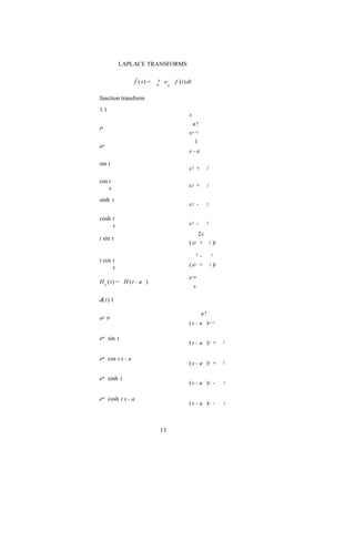
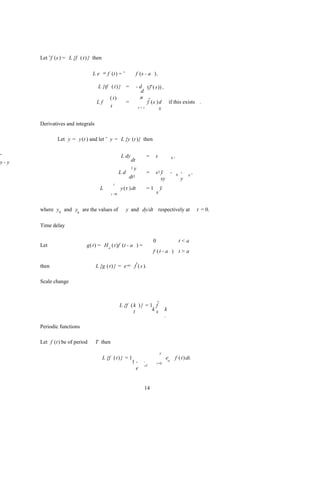
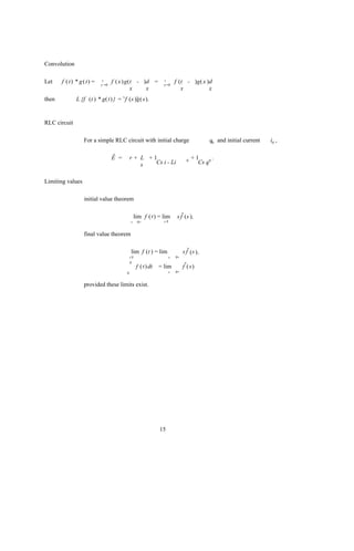
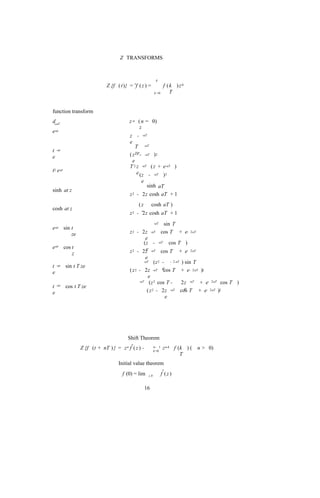
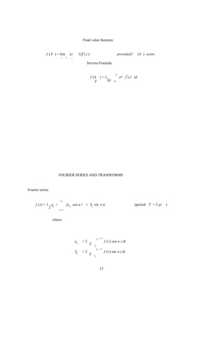
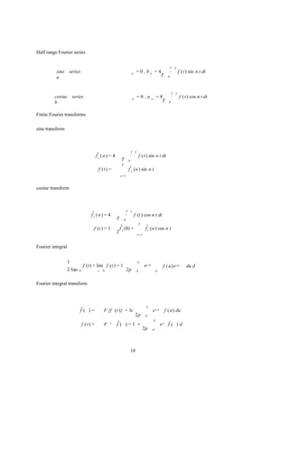
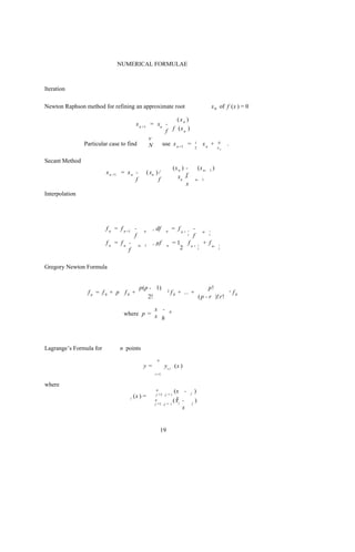
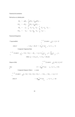
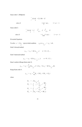
This document contains mathematical formula tables including: 1. Greek alphabet, indices and logarithms, trigonometric identities, complex numbers, hyperbolic identities, and series. 2. Derivatives of common functions, product rule, quotient rule, chain rule, and Leibnitz's theorem. 3. Integrals of common functions, double integrals, and the substitution rule for integrals.

1. LEARN MATHEMATICS
MATHEMATICAL FORMULA TABLES
1

2. 2

3. GREEK ALPHABET
A a alpha N nu
B ß beta xi
G gamma O o omicron
d delta p pi
E , epsilon P rho
e
Z zeta S s sigma
H eta T t tau
T , theta upsilon
I iota F f phi
,
K kappa X chi
lambda psi
M µ mu omega
INDICES AND LOGARITHMS
am × a n = am + n
(am ) n = a mn
log( AB ) = log A + log B
log( A/B ) = log A - log B
log( A n ) = n log A
a
log b a = log c
logc b
3

4. TRIGONOMETRIC IDENTITIES
tan A = sin A/ cos A
sec A = 1 / cos A
cosec A = 1 / sin A
cot A = cos A/ sin A = 1 / tan A
sin2 A + cos 2 A = 1
sec2 A = 1 + tan 2 A
cosec 2 A = 1 + cot 2 A
sin( A ± B ) = sin A cos B ± cos A sin B
cos( A ± B ) = cos A cos B sin A sin B
tan( A ± B ) = tan A± tan B
1 tan A tan B
sin 2A = 2 sin A cos A
cos 2A = cos 2 A - sin 2 A
= 2 cos 2 A - 1
= 1 - 2 sin2 A
tan 2 A = 2tan A
1- tan 2 A
sin 3A = 3 sin A - 4 sin3 A
cos 3A = 4 cos 3 A - 3 cos A
tan 3 A = 3 tan A- tan 3 A
1 - 3tan 2 A
sin A + sin B = 2 sin A +B cos A-B
2 2
4

5. sin A - sin B = 2 cos A+ B sin A-B
2 2
cos A + cos B = 2 cos A+ B cos A-B
2 2
cos A - cos B = - 2 sin A + B sin A-B
2 2
2 sin A cos B = sin( A + B ) + sin( A - B )
2 cos A sin B = sin( A + B ) - sin( A - B )
2 cos A cos B = cos( A + B ) + cos( A - B )
- 2 sin A sin B = cos( A + B ) - cos( A - B )
v
a sin x + b cos x = R sin( x + f ), where R = a 2 + b2 and cos f = a/R , sin f = b/R .
If t = tan 1 x then sin x = 2t , cos x = 1 -t 2 .
2 1+ t2 1+ t2
cos x = 1 ( eix + e-ix ) ; sin x = 1 (eix - -ix )
2 2i
e
eix = cos x + i sin x ; e-ix = cos x - sin x
i
5

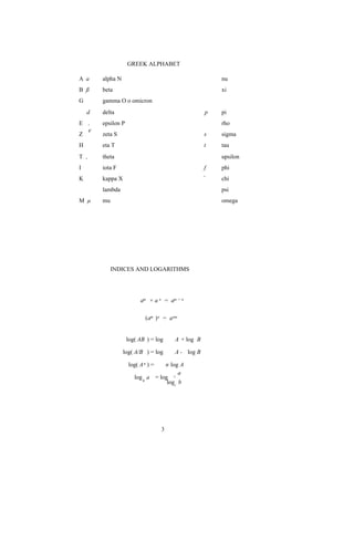
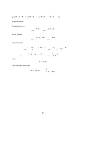
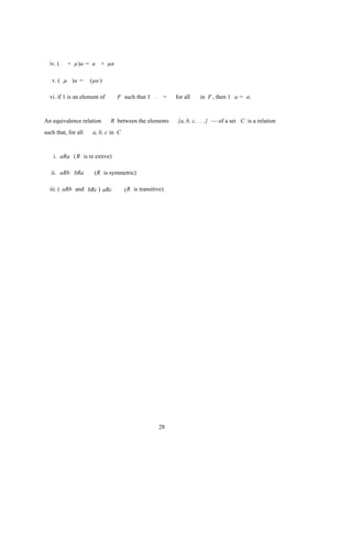
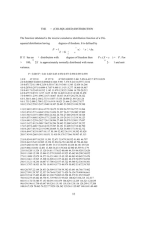
6. COMPLEX NUMBERS
v
i= - 1 Note:- ‘ j ’ often used rather than ‘ i’.
Exponential Notation
ei = cos + i sin
De Moivre’s theorem
[r (cos + i sin )]n = rn (cos n + i sin n )
nth roots of complex numbers
If z = r i = r (cos + i sin ) then
e
vr
z 1/n = ne
i ( +2 kp ) /n , = 0 , ± 1, ± 2, ...
k
HYPERBOLIC IDENTITIES
cosh x = ( ex + e-x ) / 2 sinh x = ( ex - -x )/2
e
tanh x = sinh x cosh x
/
sech x = 1 / cosh x cosech x = 1 / sinh x
coth x = cosh x sinh x = 1 / tanh x
/
cosh i = cos x sinh i = i sin x
x x
cos i = cosh x sin i = i sinh x
x x
cosh 2 A - sinh 2 A = 1
sec 2 A = 1 - tanh 2 A
h
cosec 2 A = coth 2 A - 1
h
6

7. SERIES
Powers of Natural Numbers
n n n
k = 1 n ( n + 1) ; k = 1 n ( n + 1)(2 n + 1);
2 k3 = 1 n 2 (n + 1) 2
2 6 4
k =1 k =1 k =1
n- 1 n
Arithmetic Sn = (a + k ) = { 2a + ( n - 1)d}
d 2
k =0
Geometric (convergent for - 1 < r < 1)
n- 1 a(1 - n ) a
Sn = a k = =
r 1rr,S
- 8
1-
k =0
r
Binomial (convergent for |x| 1)
<
n! n!
(1 + x )n = 1 + n + x 2 + ... + x r + ...
x ( n - 2)!2! ( n - r )!r!
n! n ( n - 1)( n - 2)... ( n - r + 1)
where
(n - r )!r ! = r!
Maclaurin series
x2 xk
f (x ) = f (0) + x (0) + f (0) + ... + f ( k ) (0) + R k +1
f 2! k!
x k +1
where R k +1 = f ( k +1) ( x ) , 0 < < 1
( k + 1)!
Taylor series
h2 hk
f ( a + h ) = f ( a) + hf ( a) + f ( a) + ... + f ( k ) (a ) + R k +1
2! k!
h k +1
where R k +1 = f ( k +1) (a + h ) , 0 < < 1.
(k + 1)!
OR
x - 0 )2 x - 0 )k ( k )
f (x ) = f ( x0 ) + ( x - 0 ) f (x 0 ) + ( x f (x 0 ) + ... + ( x f (x 0 ) + R k +1
x 2! k!
x - 0 ) k +1 ( k +1)
where R k +1 = ( x f (x 0 + ( x - 0
) ), 0 < < 1
( k + 1)! x
7

8. Special Power Series
x2 x3 xr
e =1+ x +
x ... + ... (all x )
2! + 3! + r! +
3 x5 7 - 1)r x2 r +1
sin x = x - - ... + ( ... (all x )
x 3! + 5! x 7! + (2 r + 1)! +
x4 62 - 1) r x 2r
cos x = 1 - - ... + ( ... (all x )
x 2! + 4! x 6! + (2r )! +
x3 x5 x7
tan x = x + ... ( |x| p )
3 + 2 15 + 17315 + <
2
x3 .3 x5 .3.5 x7
sin - 1 x = x +1
2 3 + 1 2. 4 5 + 1 2.4.6 7 +
.3.5.... (2 n - 1) x 2n +1
... + 1 ... ( |x| 1)
2.4. 6.... (2 n ) 2n + 1 + <
x5 3 7 x2 n +1
tan - 1 x = x - - ... + ( - 1) n ... ( |x| 1)
x 3+ 5 x 7+ 2n + 1 + <
x3 2 4 xn
n (1 + x ) = x - - ... + ( - 1) n +1 + ... ( - 1 < x = 1)
x 2+ 3 x 4+ n
x3 x5 x7 x 2 n +1
sinh x = x + ... + ... (all x )
3! + 5! + 7! + (2n + 1)! +
x2 x4 x6 x 2n
cosh x = 1 + ... + ... (all x )
2! + 4! + 6! + (2n )! +
x5 17x 7
3
tanh x = x - - ... ( |x| p )
x 3 + 2 15 315 + <
2
1 x3 .3 x5 1.3.5 x 7
sinh - 1 x = x -
- 2 3 + 1 2.4 5 2.4.6 7 +
1.3.5... (2n - 1) x2n +1
... + ( - 1) n ... ( |x| 1)
2.4.6... 2n 2n + 1 + <
x3 x5 x7 2 n +1
tanh - 1 x = x+ ... x ... ( |x| 1)
3+ 5+ 7+ 2n + 1 + <
8

9. DERIVATIVES
function derivative
xn n n- 1
xx
ex e
ax ( a > 0) ax na
n 1
x
x
loga x 1
x na
sin x cos x
cos x - sin x
tan x sec2 x
cosec x - cosec x cot x
sec x sec x tan x
cot x - cosec 2 x
1
sin- 1 x v
1- 2
x
1
cos- 1 x - v
1- 2
x
1
tan - 1 x
1 + x2
sinh x cosh x
cosh x sinh x
tanh x sech 2 x
cosech x - cosech x coth x
sech x - sech x tanh x
coth x - cosech 2 x
1
sinh - 1
x v
1 + x2
cosh - 1
x (x > 1) 1 v
x 2 - 1
tanh - 1 x ( |x| 1) 1
< 1- 2
x
1
coth - 1 x (|x| 1) -
> x2 - 1
9

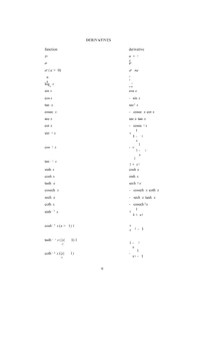
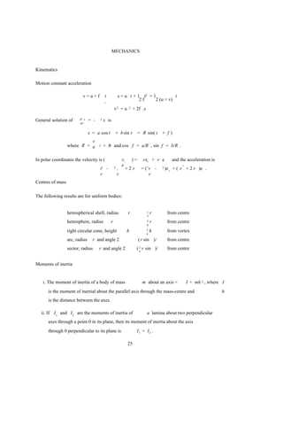
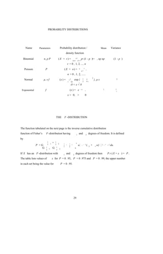
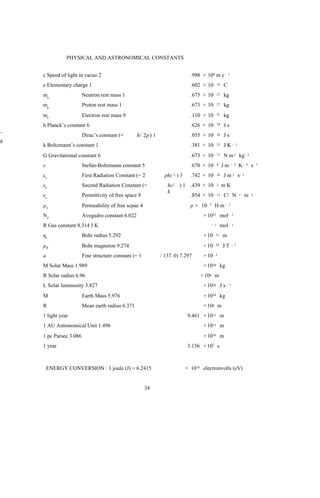
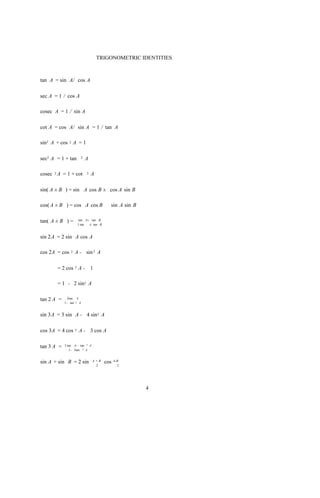
10. Product Rule
d d du
( u( x )v ( x )) = u ( x) v + v( x )
d d d
x x x
Quotient Rule
d u (x ) v ( x ) du - u ( x ) dv
dx dx
d v(x ) = [v ( x)]2
x
Chain Rule
d
(f ( g( x))) = f (g( x )) × g (x )
d
x
Leibnitz’s theorem
dn n (n - 1) n!
( f.g ) = f ( n ) .g + nf ( n- 1) .g(1) + f ( n- 2) .g (2) + ... + f ( n-r ) .g( r ) + ... + f .g ( n )
d n 2! ( n - r )!r!
x
10

11. INTEGRALS
function integral
dg(x ) (x )
f (x ) (x ) g(x ) - df ( x )d
dx f dx g x
xn (n = - 1) xn +1
n +1
1 n| Note:- n| + K = n|x/ 0 |
x
x| x| x
ex ex
sin x cos x
-
cos x sin x
tan x n| sec x
|
cosec x - n| cosec x + cot x or n tan x
2
|
sec x n| sec x + tan x = n tan p + x
4 2
|
cot x n| sin x
1 1 | x
tan - 1
a2 + x 2 a a
1 1 + x x
or 1 tanh - 1 ( |x| < a )
a2 - 2 2a n aa - x a a
x
1 1 1 x
or - coth - 1 (|x| > a )
x2 - a 2 2a n xx- + a
a a a
1 x
v sin- 1 ( a > |x| )
a 2 - 2 a
x
1 x v
v sinh - 1
or nx + x 2 + a2
a 2 + x2 a
1 x v
v cosh - 1 or n| + x 2 -a 2 | ( |x| > a )
x 2 -a 2 a x
sinh x cosh x
cosh x sinh x
tanh x n cosh x
cosech x - n |cosechx + cothx| or n tanh x
2
sech x 2 tan - 1 ex
coth x n| sinh x
|
11

12. Double integral
f ( x, ) dxdy = g( r, ) J drds
y s
where
(x, ) x x
J = r s
(y ) =
r, y y
s r s
12

13. LAPLACE TRANSFORMS
f˜ ( s) = 0
8 e- f (t) dt
st
function transform
11
s
n!
tn
s n +1
1
eat
s-a
sin t
s2 + 2
cos t
s s2 + 2
sinh t
s2 - 2
cosh t
s s2 - 2
2s
t sin t
( s2 + )
2 2
-
2 2
t cos t
s ( s2 + )
2 2
e-as
H a ( t) = H ( t - a )
s
d( t) 1
n!
eat tn
( s - a ) n +1
eat sin t
( s - a )2 + 2
eat cos t s - a
( s - a )2 + 2
eat sinh t
( s - a )2 - 2
eat cosh t s - a
( s - a )2 - 2
13

14. Let ˜f (s ) = L {f ( t) } then
Le at f (t) = ˜ f (s - a ) ,
L {tf ( t) } = - d ( f˜ ( s)) ,
d
( t) 8s
Lf = f˜ (x ) d if this exists .
t x=s x
Derivatives and integrals
Let y = y (t ) and let ˜ y = L {y (t )} then
˜ L dy = s 0 ,
y-y dt
2 y
Ld = s2 y -
˜ 0
- 0
,
dt 2
sy y
t
L y ( t ) dt =1 y
˜
t =0 s
where y0 and y0 are the values of y and dy/dt respectively at t = 0.
Time delay
0 t<a
Let g( t) = H a ( t)f (t - a ) =
f (t - a ) t > a
then L {g ( t) } = e-as f˜ ( s ).
Scale change
L {f ( k ) } = 1 f˜
t ks k
.
Periodic functions
Let f (t) be of period T then
T
L {f ( t) } = 1 e- f ( t) dt.
1- - t =0
st
sT
e
14

15. Convolution
Let f ( t) * g ( t) = t
x =0
f ( x ) g(t - )d = t
x =0
f (t - )g( x )d
x x x x
then L {f (t ) * g( t) } = ˜f (s )˜ ( s).
g
RLC circuit
For a simple RLC circuit with initial charge q0 and initial current i0 ,
˜
E = r + L +1 +1 .
0
s Cs i - Li Cs q0
Limiting values
initial value theorem
lim f ( t) = lim s f˜ (s ),
t 0+ s8
final value theorem
lim f (t ) = lim s f˜ ( s ) ,
t8 s 0+
8
f ( t) dt = lim f˜ ( s)
0 s 0+
provided these limits exist.
15

16. Z TRANSFORMS
8
Z {f ( t)} = ˜f ( z ) = f ( k ) z-k
k =0 T
function transform
dt,nT z -n ( n = 0)
z
e-at
z - -aT
e
T -aT
t -at
e ( z ze- -aT ) 2
e
T 2 z -aT ( z + e-aT )
t2 e-at e (z - -aT ) 3
e
sinh aT
sinh at z
z 2 - 2z cosh aT + 1
( z cosh aT )
cosh at z
z 2 - -2z cosh aT + 1
-aT sin T
e-at sin t
ze z 2 - 2z -aT cos T + e- 2aT
e
(z - -aT cos T )
e-at cos t e
z z 2 - 2z -aT cos T + e- 2aT
e
-aT (z 2 - - 2 aT ) sin T
t -at sin t T ze
e ( z 2 - 2z -aT e T + e- 2 aT )2
cos
e
-aT (z 2 cos T - 2z -aT + e- 2 aT cos T )
t -at cos t T ze e
e ( z 2 - 2z -aT cos T + e- 2 aT )2
e
Shift Theorem
Z {f (t + nT ) } = z n f˜ ( z ) - n- 1
k =0
z n-k f (k ) ( n > 0)
T
Initial value theorem
f (0) = lim z8 f˜ ( z )
16

17. Final value theorem
f ( 8 ) = lim (z 1) f˜ ( z ) provided f (8 ) exists
z 1
- .
Inverse Formula
p
f (k ) = 1 eik f˜ ( ei )d
T 2p -p
FOURIER SERIES AND TRANSFORMS
Fourier series
8
f ( t) = 1 a0 + {a n cos n t + bn sin n t} (period T = 2 p/ )
2
n =1
where
t0 + T
an =2 f ( t) cos n t dt
T t0
t0 + T
bn =2 f ( t) sin n t dt
T t0
17

18. Half range Fourier series
T 2
sine series n = 0 ,bn = 4 / f ( t) sin n t dt
a T 0
T 2
cosine series n
=0 ,an =4 / f ( t) cos n t dt
b T 0
Finite Fourier transforms
sine transform
T 2
f˜s ( n ) = 4 / f ( t) sin n t dt
T 0
8
f ( t) = f˜s (n ) sin n t
n =1
cosine transform
T 2
f˜c ( n ) = 4 / f (t ) cos n t dt
T 0
8
f (t ) = 1 f˜c (0) + f˜c (n ) cos n t
2 n =1
Fourier integral
1 8
f (t) + lim f ( t ) = 1 ei t 8 f ( u) e-i u du d
2 lim
t 0 t 0 2p -8 -8
Fourier integral transform
8
f˜ ( ) = F {f (t )} = 1v e-i u f ( u) du
2p -8
8
f ( t) = F- 1 f˜ ( ) = 1 v ei t f˜ ( ) d
2p -8
18

19. NUMERICAL FORMULAE
Iteration
Newton Raphson method for refining an approximate root x 0 of f (x ) = 0
(xn )
x n +1 = xn -
f f (x n )
v
Particular case to find N use x n +1 = 1 xn + N .
2 xn
Secant Method
(x n ) - (x n- 1 )
x n +1 = x n - ( xn ) /
f f xn f - n- 1
x
Interpolation
f n = f n +1 - n
, df n
= fn+ 1
- n- 1
f 2
f 2
f n = f n - n- 1
, µf n
= 1 fn+ 1
+ f n- 1
f 2 2 2
Gregory Newton Formula
p(p - 1) p!
fp = f0 + p f0 + 2 f 0 + ... + r f0
2! ( p - r )!r!
x - 0
where p = x
h
Lagrange’s Formula for n points
n
y= yi i (x )
i =1
where
n
j =1 ,j = i
(x - j )
i (x ) = x
n
j =1 ,j = i
( xi - j
)
x
19

20. Numerical di erentiation
Derivatives at a tabular point
1 3
hf 0 = µdf 0 - µd f 0 + 1 µd5 f 0 - ...
6 30
1 4
h2 f 0 = d2 f 0 - d f 0 + 1 d6 f 0 - ...
12 90
1 2 1 4
hf 0 = f0 - f0 + 1 3f0 - f0 + 1 5 f 0 - ...
2 3 4 5
5 5
h2 f 0 = 2 f -
0
3 f + 11
0
4 f
0
- f 0 + ...
12 6
Numerical Integration
x0 + h
T rapeziumRule f ( x ) dx h f0 + f1 ) + E
x0 2(
3
where f i
= f (x 0 + ih ), E = -h f ( a), 0
<a<x 0
+ h
12 x
Composite Trapezium Rule
x0 + nh 2 h4
f (x )dx h { 0
+ 2 f 1 + 2 f 2 + ...2f n- 1
+ fn } - h f - )+ f - ) ...
x0 2f 12 ( n f 0 720 ( n f 0
where f 0 = f (x 0 ), f n
= f ( x0 + nh ), etc
x 0 +2 h
Simpson sRule f ( x) dx h f 0 +4 f 1 + f 2 )+ E
x0 3(
5
wher E = -h f (4) ( a) x0 < a < x 0
+ 2 h.
e 90
Composite Simpson’s Rule ( n even)
x0 + nh
f (x )dx h f 0 + 4 f 1 + 2 f 2 + 4 f 3 + 2 f 4 + ... + 2 f n- 2 + 4 f n- 1 + fn ) + E
x0 3(
5
where E = -nh f (4) ( a) . 0
<a<x 0
+ nh
180 x
20

21. Gauss order 1. (Midpoint)
1
f (x )d = 2 f (0) + E
- 1 x
where E = 2 f (a) . - 1 <a< 1
3
Gauss order 2.
1 1 1
f (x ) d = f v f v E
- 1 x - 3+ 3+
where E =1 f v ( a) . - 1<a< 1
135
Di erential Equations
To solve y = f ( x, ) given initial condition y0 at x0 , n
= x 0 + nh .
y x
Euler’s forward method
yn +1 = yn + hf (x n , n ) n = 0 , 1, 2, ...
y
Euler’s backward method
yn +1 = yn + hf ( xn +1 , n +1 ) n = 0 , 1, 2, ...
y
Heun’s metho d (Runge Kutta order 2)
h
yn +1 = yn + f (x n , n
) + f ( xn + h, y n + hf (x n , n
))) .
2( y y
Runge Kutta order 4.
h
yn +1 = yn + K + 2 K2 + 2 K3 + K4 )
6( 1
where
K1 = f (x n , n )
y h hK 1
K2 = f n
+ , n
+
x 2y 2
h hK 2
K3 = f n
+ , n
+
x 2y 2
K4 = f (x n + h, y n + hK 3 )
21

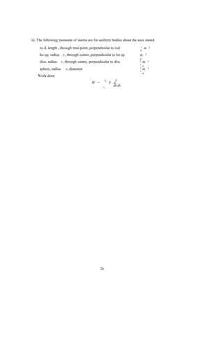
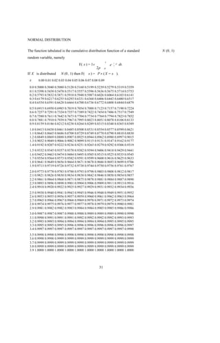
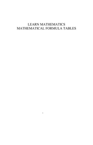
22. Chebyshev Polynomials
Tn (x ) = cos n (cos - 1 x)
To (x ) = 1 T1 ( x ) = x
Tn (x ) n (cos - 1 x)]
Un- 1
(x ) = = sin [ v
n 1- 2
x
Tm (Tn (x )) = Tmn ( x ) .
Tn +1 ( x ) = 2 x n ( x ) - T n- 1 (x )
T
Un +1 ( x ) = 2 x n ( x) - U n- 1 (x )
U T (x ) (x )
n +1
Tn ( x )d =1 - T n- 1 constant, n = 2
x 2 n +1 n- 1+
f ( x ) = 1 a0 T0 ( x ) + a1 T1 ( x ) ...a j Tj ( x) + ...
2
p
where a j
=2 f (cos ) cos j d j = 0
p 0
and f ( x ) d = constant + A 1 T1 ( x ) + A2 T2 (x ) + ...A j Tj ( x ) + ...
x
where A j = ( aj- 1
-a j +1
) / 2j j = 1
22

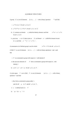
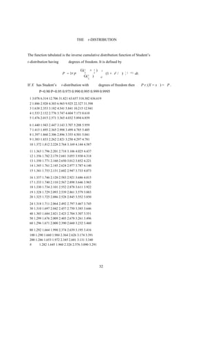
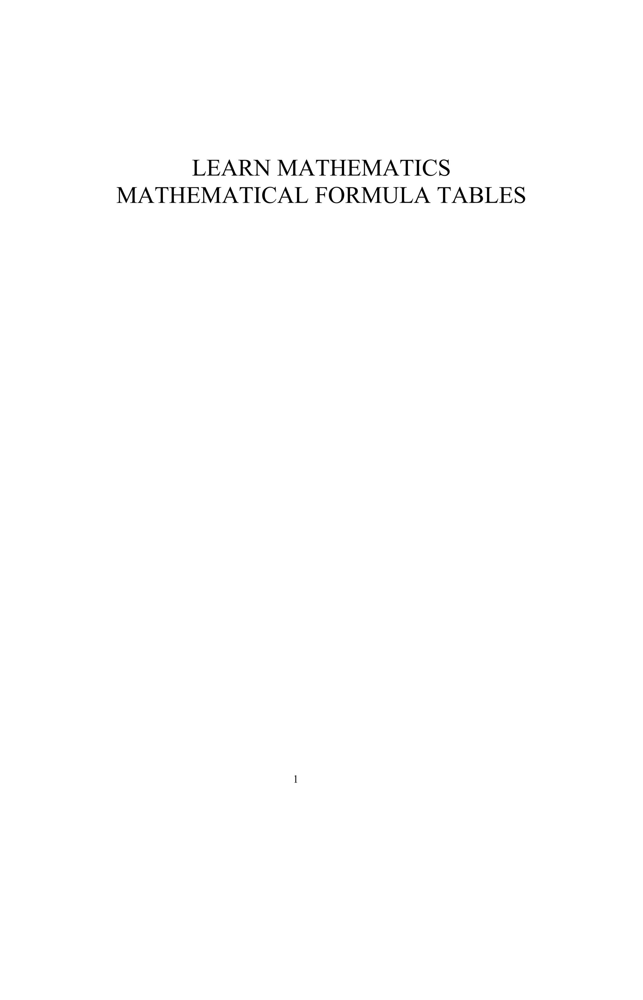
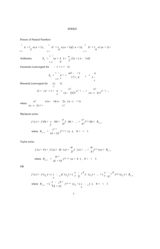
23. VECTOR FORMULAE
Scalar product a .b = ab cos = a1 b1 + a2 b2 + a3 b3
ijk
Vector product a × b = ab sin n =
ˆ a1 a2 a3
b1 b2 b3
= ( a2 b3 - a 3 2
b )i + ( a3 b1 - a 1 b3 )j + ( a1 b2 - a 2
b1 )k
Triple products
a1 a2 a3
[a , b , c] = (a × b) .c = a .(b × c) = b1 b2 b3
c1 c2 c3
a × (b × c) = (a .c)b - (a .b)c
Vector Calculus
=
x y z
, ,
grad f = f, div A = . A , curl A = × A
div grad f=. ( f)= 2 f (for scalars only)
div curl A = 0 curl grad f= 0
2 A = grad div A - curl curl A
(aß ) = a ß + ßa
div ( a A) = a div A + A . ( a )
curl ( a A) = a curl A - A × ( a )
div (A × B) = B . curl A - A . curl B
curl (A × B) = A div B - B div A + (B . )A - (A . )B
23

24. grad (A .B) = A × curl B + B × curl A + (A . )B + (B . )A
Integral Theorems
Divergence theorem
A .dS = div A dV
surface volume
Stokes’ theorem
( curl A) .dS = A .dr
surface contour
Green’s theorems
( 2 f - 2 )dV = f S|
volume f surface n-f n |d
2 f +( f )( ) dV = f S|
volume surface n |d
where
dS = ˆ n |dS |
Green’s theorem in the plane
Q
( P dx + Qdy ) =
x - P y dxdy
24

25. MECHANICS
Kinematics
Motion constant acceleration
v=u+f t s = u t + 1 t2 = 1 t
, 2f 2 (u + v)
v2 = u 2 + 2f .s
General solution of d2 x = - 2 x is
dt 2
x = a cos t + b sin t = R sin( t + f)
v
where R = a 2 + b and cos f = a/R , sin f = b/R .
2
In polar coordinates the velocity is ( r, )= rer + r e and the acceleration is
r
¨
r -
¨ 2 , +2 r = (¨r - 2 )e r + ( r ¨ + 2 r )e .
r r r
Centres of mass
The following results are for uniform bodies:
hemispherical shell, radius r 1 r from centre
2
hemisphere, radius r 3 r from centre
8
right circular cone, height h 3 h from vertex
4
arc, radius r and angle 2 ( r sin )/ from centre
sector, radius r and angle 2 ( 2 r sin )/ from centre
3
Moments of inertia
i. The moment of inertia of a body of mass m about an axis = I + mh 2 , where I
is the moment of inertial about the parallel axis through the mass-centre and h
is the distance between the axes.
ii. If I 1 and I 2 are the moments of inertia of a lamina about two perpendicular
axes through a point 0 in its plane, then its moment of inertia about the axis
through 0 perpendicular to its plane is I1 + I2 .
25

26. iii. The following moments of inertia are for uniform bodies about the axes stated:
ro d, length , through mid-point, perpendicular to rod 1 m 2
12
ho op, radius r , through centre, perpendicular to ho op m 2
r
disc, radius r, through centre, perpendicular to disc 1 m 2
2
r
sphere, radius r, diameter 2 m 2
5
r
Work done
tB r
W = F. d
tA dt dt.
26

27. ALGEBRAIC STRUCTURES
A group G is a set of elements {a, b, c, . . .} — with a binary operation * such that
i. a * b is in G for all a, b in G
ii. a * ( b * c) = ( a * b ) * c for all a, b, c in G
iii. G contains an element e , called the identity element, such that e*a = a = a*e
for all a in G
iv. given any a in G, there exists in G an element a- 1 , called the element inverse
to a, such that a- 1 * a = e = a * a- 1 .
A commutative (or Abelian) group is one for which a * b = b * a for all a, b, in G.
A field F is a set of elements {a, b, c, . . .} — with two binary operations + and . such
that
i. F is a commutative group with respect to + with identity 0
ii. the non-zero elements of F form a commutative group with respect to . with
identity 1
iii. a.( b + c) = a.b + a.c for all a, b, c, in F .
A vector space V over a field F is a set of elements {a, b, c, . . .} — with a binary
operation + such that
i. they form a commutative group under +;
and, for all ,µ in F and all a, b, in V ,
ii. a is defined and is in V
iii. (a + b) = a + b
27

28. iv. ( + µ)a = a + µa
v. ( .µ )a = (µa )
vi. if 1 is an element of F such that 1 . = for all in F , then 1 a = a.
An equivalence relation R between the elements {a, b, c, . . .} — of a set C is a relation
such that, for all a, b, c in C
i. aRa ( R is re extive)
ii. aRb bRa (R is symmetric)
iii. ( aRb and bRc ) aRc ( R is transitive).
28

29. PROBABILITY DISTRIBUTIONS
Name Parameters Probability distribution / Mean Variance
density function
Binomial n, p P (X = r) = n! pr (1 - p )n-r , np np (1 - p )
( n-r )! r !
r = 0 , 1, 2, ..., n
Poisson P (X = n) = e- n
,
n!
n = 0 , 1, 2, ......
2
Normal µ, s f (x ) = v1 exp { 1 x-
µs
}, µ s 2
s 2p 2
-
-8 < x < 8
Exponential f (x ) = e -x , 1 1
2
x > 0, > 0
THE F -DISTRIBUTION
The function tabulated on the next page is the inverse cumulative distribution
function of Fisher’s F -distribution having 1
and 2
degrees of freedom. It is defined
by
1
1
+ 1
2 1 1 x
2 2
P =G 2
1
1 2
2
2
u1
2 1 - 1 ( 2
+ 1
u) - 1
2
( 1 + 2 ) du.
G 1
1 G 1
2 0
2 2
If X has an F -distribution with 1
and 2
degrees of freedom then P r.( X = x ) = P .
The table lists values of x for P = 0 . 95, P = 0 .975 and P = 0 .99, the upper number
in each set being the value for P = 0 .95.
29

30. 2 1
:1 1
: 2 3 4 5 6 7 8 9 10 12 15 20 25 50 100
161 199 216 225 230 234 237 239 241 242 244 246 248 249 252 253
1 648 799 864 900 922 937 948 957 963 969 977 985 993 998 1008 1013 1
4052 5000 5403 5625 5764 5859 5928 5981 6022 6056 6106 6157 6209 6240 6303 6334
18.51 19.00 19.16 19.25 19.30 19.33 19.35 19.37 19.38 19.40 19.41 19.43 19.45 19.46 19.48 19.49
2 38.51 39.00 39.17 39.25 39.30 39.33 39.36 39.37 39.39 39.40 39.41 39.43 39.45 39.46 39.48 39.49 2
98.50 99.00 99.17 99.25 99.30 99.33 99.36 99.37 99.39 99.40 99.42 99.43 99.45 99.46 99.48 99.49
10.13 9.55 9.28 9.12 9.01 8.94 8.89 8.85 8.81 8.79 8.74 8.70 8.66 8.63 8.58 8.55
3 17.44 16.04 15.44 15.10 14.88 14.73 14.62 14.54 14.47 14.42 14.34 14.25 14.17 14.12 14.01 13.96 3
34.12 30.82 29.46 28.71 28.24 27.91 27.67 27.49 27.35 27.23 27.05 26.87 26.69 26.58 26.35 26.24
7.71 6.94 6.59 6.39 6.26 6.16 6.09 6.04 6.00 5.96 5.91 5.86 5.80 5.77 5.70 5.66
4 12.22 10.65 9.98 9.60 9.36 9.20 9.07 8.98 8.90 8.84 8.75 8.66 8.56 8.50 8.38 8.32 4
21.20 18.00 16.69 15.98 15.52 15.21 14.98 14.80 14.66 14.55 14.37 14.20 14.02 13.91 13.69 13.58
6.61 5.79 5.41 5.19 5.05 4.95 4.88 4.82 4.77 4.74 4.68 4.62 4.56 4.52 4.44 4.41
5 10.01 8.43 7.76 7.39 7.15 6.98 6.85 6.76 6.68 6.62 6.52 6.43 6.33 6.27 6.14 6.08 5
16.26 13.27 12.06 11.39 10.97 10.67 10.46 10.29 10.16 10.05 9.89 9.72 9.55 9.45 9.24 9.13
5.99 5.14 4.76 4.53 4.39 4.28 4.21 4.15 4.10 4.06 4.00 3.94 3.87 3.83 3.75 3.71
6 8.81 7.26 6.60 6.23 5.99 5.82 5.70 5.60 5.52 5.46 5.37 5.27 5.17 5.11 4.98 4.92 6
13.75 10.92 9.78 9.15 8.75 8.47 8.26 8.10 7.98 7.87 7.72 7.56 7.40 7.30 7.09 6.99
5.59 4.74 4.35 4.12 3.97 3.87 3.79 3.73 3.68 3.64 3.57 3.51 3.44 3.40 3.32 3.27
7 8.07 6.54 5.89 5.52 5.29 5.12 4.99 4.90 4.82 4.76 4.67 4.57 4.47 4.40 4.28 4.21 7
12.25 9.55 8.45 7.85 7.46 7.19 6.99 6.84 6.72 6.62 6.47 6.31 6.16 6.06 5.86 5.75
5.32 4.46 4.07 3.84 3.69 3.58 3.50 3.44 3.39 3.35 3.28 3.22 3.15 3.11 3.02 2.97
8 7.57 6.06 5.42 5.05 4.82 4.65 4.53 4.43 4.36 4.30 4.20 4.10 4.00 3.94 3.81 3.74 8
11.26 8.65 7.59 7.01 6.63 6.37 6.18 6.03 5.91 5.81 5.67 5.52 5.36 5.26 5.07 4.96
5.12 4.26 3.86 3.63 3.48 3.37 3.29 3.23 3.18 3.14 3.07 3.01 2.94 2.89 2.80 2.76
9 7.21 5.71 5.08 4.72 4.48 4.32 4.20 4.10 4.03 3.96 3.87 3.77 3.67 3.60 3.47 3.40 9
10.56 8.02 6.99 6.42 6.06 5.80 5.61 5.47 5.35 5.26 5.11 4.96 4.81 4.71 4.52 4.41
4.96 4.10 3.71 3.48 3.33 3.22 3.14 3.07 3.02 2.98 2.91 2.85 2.77 2.73 2.64 2.59
10 6.94 5.46 4.83 4.47 4.24 4.07 3.95 3.85 3.78 3.72 3.62 3.52 3.42 3.35 3.22 3.15 10
10.04 7.56 6.55 5.99 5.64 5.39 5.20 5.06 4.94 4.85 4.71 4.56 4.41 4.31 4.12 4.01
4.75 3.89 3.49 3.26 3.11 3.00 2.91 2.85 2.80 2.75 2.69 2.62 2.54 2.50 2.40 2.35
12 6.55 5.10 4.47 4.12 3.89 3.73 3.61 3.51 3.44 3.37 3.28 3.18 3.07 3.01 2.87 2.80 12
9.33 6.93 5.95 5.41 5.06 4.82 4.64 4.50 4.39 4.30 4.16 4.01 3.86 3.76 3.57 3.47
4.54 3.68 3.29 3.06 2.90 2.79 2.71 2.64 2.59 2.54 2.48 2.40 2.33 2.28 2.18 2.12
15 6.20 4.77 4.15 3.80 3.58 3.41 3.29 3.20 3.12 3.06 2.96 2.86 2.76 2.69 2.55 2.47 15
8.68 6.36 5.42 4.89 4.56 4.32 4.14 4.00 3.89 3.80 3.67 3.52 3.37 3.28 3.08 2.98
4.35 3.49 3.10 2.87 2.71 2.60 2.51 2.45 2.39 2.35 2.28 2.20 2.12 2.07 1.97 1.91
20 5.87 4.46 3.86 3.51 3.29 3.13 3.01 2.91 2.84 2.77 2.68 2.57 2.46 2.40 2.25 2.17 20
8.10 5.85 4.94 4.43 4.10 3.87 3.70 3.56 3.46 3.37 3.23 3.09 2.94 2.84 2.64 2.54
4.24 3.39 2.99 2.76 2.60 2.49 2.40 2.34 2.28 2.24 2.16 2.09 2.01 1.96 1.84 1.78
25 5.69 4.29 3.69 3.35 3.13 2.97 2.85 2.75 2.68 2.61 2.51 2.41 2.30 2.23 2.08 2.00 25
7.77 5.57 4.68 4.18 3.85 3.63 3.46 3.32 3.22 3.13 2.99 2.85 2.70 2.60 2.40 2.29
4.03 3.18 2.79 2.56 2.40 2.29 2.20 2.13 2.07 2.03 1.95 1.87 1.78 1.73 1.60 1.52
50 5.34 3.97 3.39 3.05 2.83 2.67 2.55 2.46 2.38 2.32 2.22 2.11 1.99 1.92 1.75 1.66 50
7.17 5.06 4.20 3.72 3.41 3.19 3.02 2.89 2.78 2.70 2.56 2.42 2.27 2.17 1.95 1.82
3.94 3.09 2.70 2.46 2.31 2.19 2.10 2.03 1.97 1.93 1.85 1.77 1.68 1.62 1.48 1.39
100 5.18 3.83 3.25 2.92 2.70 2.54 2.42 2.32 2.24 2.18 2.08 1.97 1.85 1.77 1.59 1.48 100
6.90 4.82 3.98 3.51 3.21 2.99 2.82 2.69 2.59 2.50 2.37 2.22 2.07 1.97 1.74 1.60
30

31. NORMAL DISTRIBUTION
The function tabulated is the cumulative distribution function of a standard N (0, 1)
random variable, namely
x
F( x ) = 1v e-
1
2
t2 dt.
2p -8
If X is distributed N (0 , 1) then F( x ) = P r.( X = x ).
x 0.00 0.01 0.02 0.03 0.04 0.05 0.06 0.07 0.08 0.09
0.0 0.5000 0.5040 0.5080 0.5120 0.5160 0.5199 0.5239 0.5279 0.5319 0.5359
0.1 0.5398 0.5438 0.5478 0.5517 0.5557 0.5596 0.5636 0.5675 0.5714 0.5753
0.2 0.5793 0.5832 0.5871 0.5910 0.5948 0.5987 0.6026 0.6064 0.6103 0.6141
0.3 0.6179 0.6217 0.6255 0.6293 0.6331 0.6368 0.6406 0.6443 0.6480 0.6517
0.4 0.6554 0.6591 0.6628 0.6664 0.6700 0.6736 0.6772 0.6808 0.6844 0.6879
0.5 0.6915 0.6950 0.6985 0.7019 0.7054 0.7088 0.7123 0.7157 0.7190 0.7224
0.6 0.7257 0.7291 0.7324 0.7357 0.7389 0.7422 0.7454 0.7486 0.7517 0.7549
0.7 0.7580 0.7611 0.7642 0.7673 0.7704 0.7734 0.7764 0.7794 0.7823 0.7852
0.8 0.7881 0.7910 0.7939 0.7967 0.7995 0.8023 0.8051 0.8078 0.8106 0.8133
0.9 0.8159 0.8186 0.8212 0.8238 0.8264 0.8289 0.8315 0.8340 0.8365 0.8389
1.0 0.8413 0.8438 0.8461 0.8485 0.8508 0.8531 0.8554 0.8577 0.8599 0.8621
1.1 0.8643 0.8665 0.8686 0.8708 0.8729 0.8749 0.8770 0.8790 0.8810 0.8830
1.2 0.8849 0.8869 0.8888 0.8907 0.8925 0.8944 0.8962 0.8980 0.8997 0.9015
1.3 0.9032 0.9049 0.9066 0.9082 0.9099 0.9115 0.9131 0.9147 0.9162 0.9177
1.4 0.9192 0.9207 0.9222 0.9236 0.9251 0.9265 0.9279 0.9292 0.9306 0.9319
1.5 0.9332 0.9345 0.9357 0.9370 0.9382 0.9394 0.9406 0.9418 0.9429 0.9441
1.6 0.9452 0.9463 0.9474 0.9484 0.9495 0.9505 0.9515 0.9525 0.9535 0.9545
1.7 0.9554 0.9564 0.9573 0.9582 0.9591 0.9599 0.9608 0.9616 0.9625 0.9633
1.8 0.9641 0.9649 0.9656 0.9664 0.9671 0.9678 0.9686 0.9693 0.9699 0.9706
1.9 0.9713 0.9719 0.9726 0.9732 0.9738 0.9744 0.9750 0.9756 0.9761 0.9767
2.0 0.9773 0.9778 0.9783 0.9788 0.9793 0.9798 0.9803 0.9808 0.9812 0.9817
2.1 0.9821 0.9826 0.9830 0.9834 0.9838 0.9842 0.9846 0.9850 0.9854 0.9857
2.2 0.9861 0.9864 0.9868 0.9871 0.9875 0.9878 0.9881 0.9884 0.9887 0.9890
2.3 0.9893 0.9896 0.9898 0.9901 0.9904 0.9906 0.9909 0.9911 0.9913 0.9916
2.4 0.9918 0.9920 0.9922 0.9925 0.9927 0.9929 0.9931 0.9932 0.9934 0.9936
2.5 0.9938 0.9940 0.9941 0.9943 0.9945 0.9946 0.9948 0.9949 0.9951 0.9952
2.6 0.9953 0.9955 0.9956 0.9957 0.9959 0.9960 0.9961 0.9962 0.9963 0.9964
2.7 0.9965 0.9966 0.9967 0.9968 0.9969 0.9970 0.9971 0.9972 0.9973 0.9974
2.8 0.9974 0.9975 0.9976 0.9977 0.9977 0.9978 0.9979 0.9979 0.9980 0.9981
2.9 0.9981 0.9982 0.9982 0.9983 0.9984 0.9984 0.9985 0.9985 0.9986 0.9986
3.0 0.9987 0.9987 0.9987 0.9988 0.9988 0.9989 0.9989 0.9989 0.9990 0.9990
3.1 0.9990 0.9991 0.9991 0.9991 0.9992 0.9992 0.9992 0.9992 0.9993 0.9993
3.2 0.9993 0.9993 0.9994 0.9994 0.9994 0.9994 0.9994 0.9995 0.9995 0.9995
3.3 0.9995 0.9995 0.9995 0.9996 0.9996 0.9996 0.9996 0.9996 0.9996 0.9997
3.4 0.9997 0.9997 0.9997 0.9997 0.9997 0.9997 0.9997 0.9997 0.9997 0.9998
3.5 0.9998 0.9998 0.9998 0.9998 0.9998 0.9998 0.9998 0.9998 0.9998 0.9998
3.6 0.9998 0.9998 0.9999 0.9999 0.9999 0.9999 0.9999 0.9999 0.9999 0.9999
3.7 0.9999 0.9999 0.9999 0.9999 0.9999 0.9999 0.9999 0.9999 0.9999 0.9999
3.8 0.9999 0.9999 0.9999 0.9999 0.9999 0.9999 0.9999 0.9999 0.9999 0.9999
3.9 1.0000 1.0000 1.0000 1.0000 1.0000 1.0000 1.0000 1.0000 1.0000 1.0000
31

32. THE t-DISTRIBUTION
The function tabulated is the inverse cumulative distribution function of Student’s
t-distribution having degrees of freedom. It is defined by
G( 1 + 1 ) x
P = 1v p 2 2 (1 + t2 / )- 1
2
( +1) dt.
G( 1 ) -8
2
If X has Student’s t-distribution with degrees of freedom then P r. (X = x ) = P .
P=0.90 P=0.95 0.975 0.990 0.995 0.999 0.9995
1 3.078 6.314 12.706 31.821 63.657 318.302 636.619
2 1.886 2.920 4.303 6.965 9.925 22.327 31.598
3 1.638 2.353 3.182 4.541 5.841 10.215 12.941
4 1.533 2.132 2.776 3.747 4.604 7.173 8.610
5 1.476 2.015 2.571 3.365 4.032 5.894 6.859
6 1.440 1.943 2.447 3.143 3.707 5.208 5.959
7 1.415 1.895 2.365 2.998 3.499 4.785 5.405
8 1.397 1.860 2.306 2.896 3.355 4.501 5.041
9 1.383 1.833 2.262 2.821 3.250 4.297 4.781
10 1.372 1.812 2.228 2.764 3.169 4.144 4.587
11 1.363 1.796 2.201 2.718 3.106 4.025 4.437
12 1.356 1.782 2.179 2.681 3.055 3.930 4.318
13 1.350 1.771 2.160 2.650 3.012 3.852 4.221
14 1.345 1.761 2.145 2.624 2.977 3.787 4.140
15 1.341 1.753 2.131 2.602 2.947 3.733 4.073
16 1.337 1.746 2.120 2.583 2.921 3.686 4.015
17 1.333 1.740 2.110 2.567 2.898 3.646 3.965
18 1.330 1.734 2.101 2.552 2.878 3.611 3.922
19 1.328 1.729 2.093 2.539 2.861 3.579 3.883
20 1.325 1.725 2.086 2.528 2.845 3.552 3.850
24 1.318 1.711 2.064 2.492 2.797 3.467 3.745
30 1.310 1.697 2.042 2.457 2.750 3.385 3.646
40 1.303 1.684 2.021 2.423 2.704 3.307 3.551
50 1.299 1.676 2.009 2.403 2.678 3.261 3.496
60 1.296 1.671 2.000 2.390 2.660 3.232 3.460
80 1.292 1.664 1.990 2.374 2.639 3.195 3.416
100 1.290 1.660 1.984 2.364 2.626 3.174 3.391
200 1.286 1.653 1.972 2.345 2.601 3.131 3.340
8 1.282 1.645 1.960 2.326 2.576 3.090 3.291
32

33. THE 2 (CHI-SQUARED) DISTRIBUTION
The function tabulated is the inverse cumulative distribution function of a Chi-
squared distribution having degrees of freedom. It is defined by
x
P =1 u1 -
2
1 e- 1
2
u du.
2/ 2 G 1 0
2
If X has an 2 distribution with degrees of freedom then P r. (X = x ) = P . For
v v
> 100, 2X is approximately normally distributed with mean 2- 1 and unit
variance.
P = 0.005 P = 0.01 0.025 0.05 0.950 0.975 0.990 0.995 0.999
1.0 0 .04 393 0 .03 157 0 .03 982 0.00393 3.841 5.024 6.635 7.879 10.828
2.0 0.010003 0.02010 0.05064 0.1026 5.991 7.378 9.210 10.597 13.816
3.0 0.07172 0.1148 0.2158 0.3518 7.815 9.348 11.345 12.838 16.266
4.0 0.2070 0.2971 0.4844 0.7107 9.488 11.143 13.277 14.860 18.467
5.0 0.4117 0.5543 0.8312 1.145 11.070 12.832 15.086 16.750 20.515
6.0 0.6757 0.8721 1.237 1.635 12.592 14.449 16.812 18.548 22.458
7.0 0.9893 1.239 1.690 2.167 14.067 16.013 18.475 20.278 24.322
8.0 1.344 1.646 2.180 2.733 15.507 17.535 20.090 21.955 26.124
9.0 1.735 2.088 2.700 3.325 16.919 19.023 21.666 23.589 27.877
10.0 2.156 2.558 3.247 3.940 18.307 20.483 23.209 25.188 29.588
11.0 2.603 3.053 3.816 4.575 19.675 21.920 24.725 26.757 31.264
12.0 3.074 3.571 4.404 5.226 21.026 23.337 26.217 28.300 32.909
13.0 3.565 4.107 5.009 5.892 22.362 24.736 27.688 29.819 34.528
14.0 4.075 4.660 5.629 6.571 23.685 26.119 29.141 31.319 36.123
15.0 4.601 5.229 6.262 7.261 24.996 27.488 30.578 32.801 37.697
16.0 5.142 5.812 6.908 7.962 26.296 28.845 32.000 34.267 39.252
17.0 5.697 6.408 7.564 8.672 27.587 30.191 33.409 35.718 40.790
18.0 6.265 7.015 8.231 9.390 28.869 31.526 34.805 37.156 42.312
19.0 6.844 7.633 8.907 10.117 30.144 32.852 36.191 38.582 43.820
20.0 7.434 8.260 9.591 10.851 31.410 34.170 37.566 39.997 45.315
21.0 8.034 8.897 10.283 11.591 32.671 35.479 38.932 41.401 46.797
22.0 8.643 9.542 10.982 12.338 33.924 36.781 40.289 42.796 48.268
23.0 9.260 10.196 11.689 13.091 35.172 38.076 41.638 44.181 49.728
24.0 9.886 10.856 12.401 13.848 36.415 39.364 42.980 45.559 51.179
25.0 10.520 11.524 13.120 14.611 37.652 40.646 44.314 46.928 52.620
26.0 11.160 12.198 13.844 15.379 38.885 41.923 45.642 48.290 54.052
27.0 11.808 12.879 14.573 16.151 40.113 43.195 46.963 49.645 55.476
28.0 12.461 13.565 15.308 16.928 41.337 44.461 48.278 50.993 56.892
29.0 13.121 14.256 16.047 17.708 42.557 45.722 49.588 52.336 58.301
30.0 13.787 14.953 16.791 18.493 43.773 46.979 50.892 53.672 59.703
40.0 20.707 22.164 24.433 26.509 55.758 59.342 63.691 66.766 73.402
50.0 27.991 29.707 32.357 34.764 67.505 71.420 76.154 79.490 86.661
60.0 35.534 37.485 40.482 43.188 79.082 83.298 88.379 91.952 99.607
70.0 43.275 45.442 48.758 51.739 90.531 95.023 100.425 104.215 112.317
80.0 51.172 53.540 57.153 60.391 101.879 106.629 112.329 116.321 124.839
90.0 59.196 61.754 65.647 69.126 113.145 118.136 124.116 128.299 137.208
100.0 67.328 70.065 74.222 77.929 124.342 129.561 135.807 140.169 149.449
33

34. PHYSICAL AND ASTRONOMICAL CONSTANTS
c Speed of light in vacuo 2 .998 × 108 m s - 1
e Elementary charge 1 .602 × 10- 19 C
mn Neutron rest mass 1 .675 × 10- 27 kg
mp Proton rest mass 1 .673 × 10- 27 kg
me Electron rest mass 9 .110 × 10- 31 kg
h Planck’s constant 6 .626 × 10- 34 Js
¯ Dirac’s constant (= h/ 2p ) 1 .055 × 10- 34 Js
h
k Boltzmann’s constant 1 .381 × 10- 23 JK- 1
G Gravitational constant 6 .673 × 10- 11 N m 2 kg- 2
s Stefan-Boltzmann constant 5 .670 × 10- 8 Jm - 2 K- 4 s- 1
c1 First Radiation Constant (= 2 phc 2 ) 3 .742 × 10- 16 J m 2 s- 1
c2 Second Radiation Constant (= hc/ ) 1 .439 × 10- 2 mK
k
eo Permittivity of free space 8 .854 × 10- 12 C2 N- 1 m- 2
µo Permeability of free scpae 4 p × 10- 7 H m- 1
NA Avogadro constant 6.022 × 1023 mol- 1
R Gas constant 8.314 J K - 1 mol - 1
a0 Bohr radius 5.292 × 10- 11 m
µB Bohr magneton 9.274 × 10- 24 JT - 1
a Fine structure constant (= 1 / 137. 0) 7.297 × 10- 3
M Solar Mass 1.989 × 1030 kg
R Solar radius 6.96 × 108 m
L Solar luminosity 3.827 × 1026 J s - 1
M Earth Mass 5.976 × 1024 kg
R Mean earth radius 6.371 × 106 m
1 light year 9.461 × 1015 m
1 AU Astronomical Unit 1.496 × 1011 m
1 pc Parsec 3.086 × 1016 m
1 year 3.156 × 107 s
ENERGY CONVERSION : 1 joule (J) = 6.2415 × 1018 electronvolts (eV)
34