Downloaded 104 times

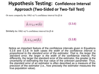
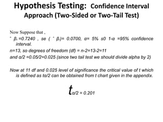
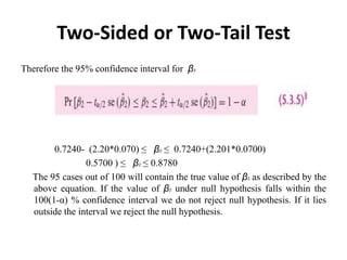
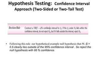
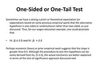
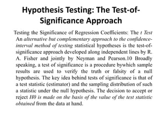
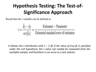
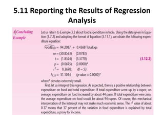

- The document discusses hypothesis testing using regression analysis, focusing on the confidence interval approach and test of significance approach. - It provides an example using wage and education data to test the hypothesis that the slope coefficient is equal to 0.5. Both the confidence interval approach and t-test approach are used to reject the null hypothesis. - One-tailed and two-tailed hypothesis tests are explained. Additional topics covered include choosing the significance level, statistical versus practical significance, and reporting the results of regression analysis.