Downloaded 288 times
![Muhammad Ali
Lecturer in Statistics
GPGC Mardan.
1
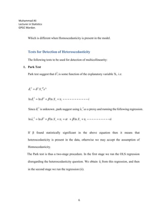
Heteroscedasticity
Definition
One of the assumption of the classical linear regression model that the error ( iε )
term having the same variance i.e. δ2
. But in most practical situation this
assumption did not fulfill, and we have the problem of heteroscedasticity.
Heteroscedasticity does not destroy the unbiased and consistency property of the
ordinary least square estimators, but these estimators have not the property of
minimum variance. Recall that OLS makes the assumption that V (εi ) =σ2 for al i.
That is, the variance of the error term is constant. (Homoscedasticity). If the error
terms do not have constant variance, they are said to be heteroscedasticity. The
term means “differing variance” and comes from the Greek “hetero” ('different')
and “scedasis” ('dispersion').]
When heteroscedasticity might occur/causes of heteroscedasticity
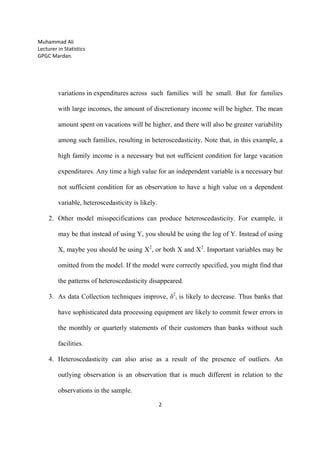
1. Errors may increase as the value of an independent variable increases. For
example, consider a model in which annual family income is the independent
variable and annual family expenditures on vacations is the dependent variable.
Families with low incomes will spend relatively little on vacations, and the](https://image.slidesharecdn.com/heteroscedasticity3-150218115247-conversion-gate01/85/Heteroscedasticity-1-320.jpg)
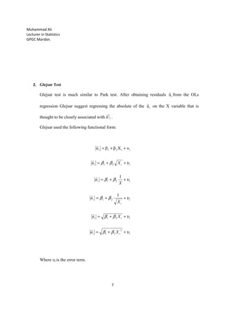
![Muhammad Ali
Lecturer in Statistics
GPGC Mardan.
1
Heteroscedasticity
Definition
One of the assumption of the classical linear regression model that the error ( iε )
term having the same variance i.e. δ2
. But in most practical situation this
assumption did not fulfill, and we have the problem of heteroscedasticity.
Heteroscedasticity does not destroy the unbiased and consistency property of the
ordinary least square estimators, but these estimators have not the property of
minimum variance. Recall that OLS makes the assumption that V (εi ) =σ2 for al i.
That is, the variance of the error term is constant. (Homoscedasticity). If the error
terms do not have constant variance, they are said to be heteroscedasticity. The
term means “differing variance” and comes from the Greek “hetero” ('different')
and “scedasis” ('dispersion').]
When heteroscedasticity might occur/causes of heteroscedasticity
1. Errors may increase as the value of an independent variable increases. For
example, consider a model in which annual family income is the independent
variable and annual family expenditures on vacations is the dependent variable.
Families with low incomes will spend relatively little on vacations, and the](https://image.slidesharecdn.com/heteroscedasticity3-150218115247-conversion-gate01/75/Heteroscedasticity-1-2048.jpg)
![Muhammad Ali
Lecturer in Statistics
GPGC Mardan.
5
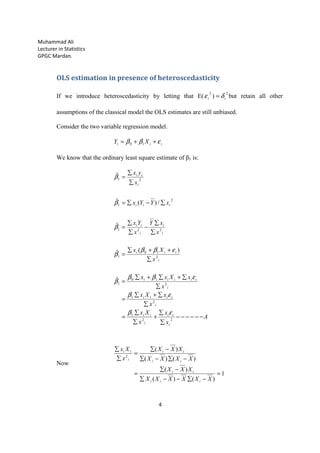
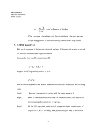
Put this value in equation (A)
Similarly 00 )ˆ( ββ =E
It is shown that in the presence of heteroscedasticity the OLS estimators are unbiased.
Variance of OLS estimator in the presence of heteroscedasticity
Since
[ ]
[ ]
[ ]
2
2
1
2
22
2
22
222
2
2
2
2
1
2
1
222
2
2
2
2
1
2
1
i
112121
222
2
2
2
2
1
2
11
2i
2
i
2
121
2
11
)ˆ(
)(
...w
)(...)()(w
0)E(thatknowwebecausezerotoequalsrmproduct tecrossThe
......)ˆVar(
wAswE
resultpreviousUsing
ˆ)ˆ(
i
i
i
i
i
ii
nn
nn
j
nnnnnn
i
i
i
i
ii
x
Var
x
x
w
ww
EwEwE
wwwwwwwE
x
x
x
x
E
EVar
∑
=
∑
∑
=∑=
++=
++=
=
++++++=
∑
=∑=
−
∑
∑
+=
−=
−−
δ
β
δδ
δδδ
εεε
εε
εεεεεεεβ
ε
β
ε
β
βββ](https://image.slidesharecdn.com/heteroscedasticity3-150218115247-conversion-gate01/85/Heteroscedasticity-5-320.jpg)


The document discusses heteroscedasticity, which occurs when the variance of the error term is not constant. It defines heteroscedasticity and provides potential causes, such as errors increasing with an independent variable or model misspecification. Consequences are that OLS estimates are no longer BLUE and standard errors are biased. Several tests for detecting heteroscedasticity are outlined, including Park, Glejser, Spearman rank correlation, and Goldfeld-Quandt tests. The Goldfeld-Quandt test involves dividing data into groups and comparing regression sum of squares to test if error variance differs between groups.