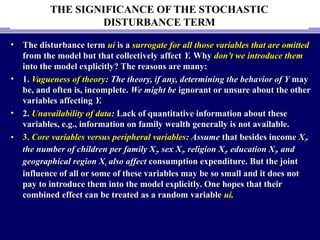
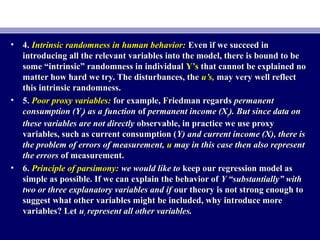
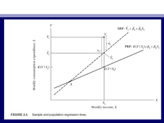
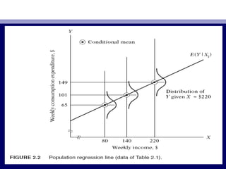
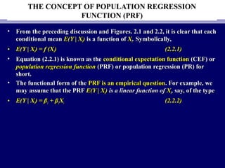
This document provides an overview of two-variable regression analysis and the concept of the population regression function. It discusses how regression analysis is used to estimate the mean value of the dependent variable based on the independent variable. It introduces a hypothetical example using family income and consumption expenditure data. It defines key concepts like the population regression line and function, and explains how the regression model specifies the dependent variable as a linear function of the independent variables plus a stochastic disturbance term to account for omitted variables.

1. 405 ECONOMETRICS
Chapter # 2: TWO-VARIABLE REGRESSION
ANALYSIS: SOME BASIC IDEAS
Domodar N. Gujarati
Prof. M. El-SakkaProf. M. El-Sakka
Dept of Economics. Kuwait UniversityDept of Economics. Kuwait University

2. A HYPOTHETICAL EXAMPLE
• Regression analysis is largely concerned with estimating and/or predictingRegression analysis is largely concerned with estimating and/or predicting
the (population)the (population) meanmean value of the dependent variable on the basis of thevalue of the dependent variable on the basis of the
known orknown or fixed values of the explanatory variable(s).fixed values of the explanatory variable(s).
• Look at table 2.1 which refers to a total population of 60 families and theirLook at table 2.1 which refers to a total population of 60 families and their
weekly income (weekly income (XX) and weekly consumption expenditure () and weekly consumption expenditure (YY). The 60). The 60
families are divided intofamilies are divided into 1010 income groups.income groups.
• There isThere is considerable variationconsiderable variation in weekly consumption expenditure in eachin weekly consumption expenditure in each
income group. But the general picture that one gets is that, despite theincome group. But the general picture that one gets is that, despite the
variability of weekly consumption expenditure within each income bracket,variability of weekly consumption expenditure within each income bracket,
on the average, weekly consumptionon the average, weekly consumption expenditureexpenditure increasesincreases as incomeas income
increases.increases.

5. • The dark circled points in Figure 2.1 show the conditional mean values ofThe dark circled points in Figure 2.1 show the conditional mean values of YY
against the various X valuesagainst the various X values.. If we join these conditional mean valuesIf we join these conditional mean values, we, we
obtain what is known asobtain what is known as the population regression line (PRL),the population regression line (PRL), or moreor more
generally, the population regression curve. More simply, it is the regressiongenerally, the population regression curve. More simply, it is the regression
ofof Y on X.Y on X. The adjectiveThe adjective “population”“population” comes from the fact that we arecomes from the fact that we are
dealing in this example with the entire population of 60 families. Of course,dealing in this example with the entire population of 60 families. Of course,
in reality a population may have many families.in reality a population may have many families.

7. THE CONCEPT OF POPULATION REGRESSION
FUNCTION (PRF)
• From the preceding discussion and Figures. 2.1 and 2.2, it is clear that eachFrom the preceding discussion and Figures. 2.1 and 2.2, it is clear that each
conditional meanconditional mean E(Y | XE(Y | Xii)) is a function ofis a function of XXii.. Symbolically,Symbolically,
• E(Y | XE(Y | Xii) = f (X) = f (Xii)) (2.2.1)(2.2.1)
• Equation (2.2.1) is known as theEquation (2.2.1) is known as the conditional expectation functionconditional expectation function (CEF) or(CEF) or
population regression functionpopulation regression function (PRF) or population regression (PR) for(PRF) or population regression (PR) for
short.short.
• The functional form of theThe functional form of the PRF is an empirical questionPRF is an empirical question. For example, we. For example, we
may assume that the PRFmay assume that the PRF E(Y | XE(Y | Xii)) is a linear function ofis a linear function of XXii,, say, of the typesay, of the type
• E(Y | XE(Y | Xii) = β) = β11 + β+ β22XXii (2.2.2)(2.2.2)

8. THE MEANING OF THE TERM LINEAR
• Linearity in the VariablesLinearity in the Variables
• The first meaning of linearity is that theThe first meaning of linearity is that the conditional expectation ofconditional expectation of Y is aY is a
linear function of Xlinear function of Xii,, the regression curve in this case is a straight line. Butthe regression curve in this case is a straight line. But
• E(Y | XE(Y | Xii) = β) = β11 + β+ β22XX22
ii is not a linear functionis not a linear function
• Linearity in the ParametersLinearity in the Parameters
• The second interpretation of linearity is that the conditional expectation ofThe second interpretation of linearity is that the conditional expectation of
Y, E(Y | XY, E(Y | Xii), is a linear function of the parameters, the β’s), is a linear function of the parameters, the β’s; it may or may not; it may or may not
be linear in the variable X.be linear in the variable X.
• E(Y | XE(Y | Xii) = β) = β11 + β+ β22XX22
ii
• is a linearis a linear (in the parameter) regression model.(in the parameter) regression model. All the models shown inAll the models shown in
Figure 2.3 are thus linear regressionFigure 2.3 are thus linear regression models, that is, models linear in themodels, that is, models linear in the
parameters.parameters.

10. • Now consider the model:Now consider the model:
• E(Y | XE(Y | Xii) = β) = β11 + β+ β22
22
XXii ..
• TheThe preceding model is an example of a nonlinear (in the parameter)preceding model is an example of a nonlinear (in the parameter)
regression model.regression model.
• From now on the term “linear” regression will always mean a regression thatFrom now on the term “linear” regression will always mean a regression that
is linear in the parametersis linear in the parameters;; the β’sthe β’s (that is, the parameters are raised to the(that is, the parameters are raised to the
first power only).first power only).

11. STOCHASTIC SPECIFICATION OF PRF
• We can express theWe can express the deviation of an individual Ydeviation of an individual Yii around its expected valuearound its expected value
as follows:as follows:
• uuii = Y= Yii − E(Y | X− E(Y | Xii))
• oror
• YYii = E(Y | X= E(Y | Xii) + u) + uii (2.4.1)(2.4.1)
• Technically,Technically, uuii is known asis known as the stochastic disturbance or stochastic error termthe stochastic disturbance or stochastic error term..
• How do we interpretHow do we interpret (2.4.1)?(2.4.1)? The expenditure of an individual family, givenThe expenditure of an individual family, given
its income level, can be expressed as the sum of two components:its income level, can be expressed as the sum of two components:
– (1)(1) E(Y | XE(Y | Xii),), the mean consumptionthe mean consumption of all families with the same level of income.of all families with the same level of income.
This component is known as theThis component is known as the systematic, or deterministic,systematic, or deterministic, componentcomponent,,
– (2)(2) uuii,, whichwhich is theis the random, or nonsystematic,random, or nonsystematic, componentcomponent..

12. • For the moment assume that the stochastic disturbance term is aFor the moment assume that the stochastic disturbance term is a proxy forproxy for
all the omitted or neglected variablesall the omitted or neglected variables that may affectthat may affect YY but are not includedbut are not included
in the regression model.in the regression model.
• IfIf E(Y | XE(Y | Xii)) is assumed to be linear inis assumed to be linear in XXii, as in (2.2.2), Eq. (2.4.1) may be, as in (2.2.2), Eq. (2.4.1) may be
written as:written as:
• YYii = E(Y | X= E(Y | Xii) + u) + uii
• == ββ11 + β+ β22XXii + u+ uii (2.4.2)(2.4.2)
• Equation (2.4.2) posits that the consumption expenditure of a family isEquation (2.4.2) posits that the consumption expenditure of a family is
linearly related to its income plus the disturbance term. Thus, thelinearly related to its income plus the disturbance term. Thus, the
individual consumption expenditures, givenindividual consumption expenditures, given X = $80X = $80 can be expressedcan be expressed as:as:
• Y1 = 55 = βY1 = 55 = β11 + β+ β22(80) + u(80) + u11
• Y2 = 60 = βY2 = 60 = β11 + β+ β22(80) + u(80) + u22
• Y3 = 65 = βY3 = 65 = β11 + β+ β22(80) + u(80) + u33 (2.4.3)(2.4.3)
• Y4 = 70 = βY4 = 70 = β11 + β+ β22(80) + u(80) + u44
• Y5 = 75 = βY5 = 75 = β11 + β+ β22(80) + u(80) + u55

13. • Now ifNow if we take the expected valuewe take the expected value of (2.4.1) on both sides, we obtainof (2.4.1) on both sides, we obtain
• E(YE(Yii | X| Xii) = E[E(Y | X) = E[E(Y | Xii)] + E(u)] + E(uii | X| Xii))
• == E(Y | XE(Y | Xii) + E(u) + E(uii | X| Xii)) (2.4.4)(2.4.4)
• Where expected value of a constant is that constant itself.Where expected value of a constant is that constant itself.
• SinceSince E(YE(Yii | X| Xii)) is the same thing asis the same thing as E(Y | XE(Y | Xii),), Eq. (2.4.4) implies thatEq. (2.4.4) implies that
• E(uE(uii | X| Xii) = 0) = 0 (2.4.5)(2.4.5)
• Thus, the assumption that the regression line passes through the conditionalThus, the assumption that the regression line passes through the conditional
means ofmeans of Y implies that theY implies that the conditional mean valuesconditional mean values ofof uuii (conditional upon(conditional upon
the giventhe given X’sX’s)) are zeroare zero..
• It is clear thatIt is clear that
• E(Y | XE(Y | Xii) = β) = β11 + β+ β22XXii (2.2.2)(2.2.2)
• andand
• YYii == ββ11 + β+ β22XXii + u+ uii (2.4.2)(2.4.2) BetterBetter
• are equivalent forms ifare equivalent forms if E(uE(uii | X| Xii) = 0.) = 0.

14. • But the stochastic specificationBut the stochastic specification (2.4.2) has the(2.4.2) has the advantage that it clearlyadvantage that it clearly
shows that there are other variables besides income that affect consumptionshows that there are other variables besides income that affect consumption
expenditure and that an individual family’s consumption expenditureexpenditure and that an individual family’s consumption expenditure
cannot be fully explained only by the variable(s) included in the regressioncannot be fully explained only by the variable(s) included in the regression
model.model.

15. THE SIGNIFICANCE OF THE STOCHASTIC
DISTURBANCE TERM
• The disturbance termThe disturbance term uiui is ais a surrogate for all those variables that are omittedsurrogate for all those variables that are omitted
from the model but that collectively affectfrom the model but that collectively affect Y.Y. WhyWhy don’t we introduce themdon’t we introduce them
into the model explicitly? The reasons are many:into the model explicitly? The reasons are many:
• 1.1. Vagueness of theoryVagueness of theory: The theory, if any, determining the behavior of Y: The theory, if any, determining the behavior of Y maymay
be, and often is, incomplete.be, and often is, incomplete. We might beWe might be ignorant or unsure about the otherignorant or unsure about the other
variables affectingvariables affecting Y.Y.
• 2.2. Unavailability of dataUnavailability of data:: Lack of quantitative information about theseLack of quantitative information about these
variables, e.g., information on family wealth generally is not available.variables, e.g., information on family wealth generally is not available.
• 3.3. Core variables versus peripheral variablesCore variables versus peripheral variables: Assume: Assume that besides incomethat besides income XX11,,
the number of children per family Xthe number of children per family X22, sex X, sex X33, religion X, religion X44, education X, education X55, and, and
geographical region Xgeographical region X66 also affectalso affect consumption expenditure. But the jointconsumption expenditure. But the joint
influence of all or some of these variables may be so small and it does notinfluence of all or some of these variables may be so small and it does not
pay to introduce them into the model explicitly. One hopes that theirpay to introduce them into the model explicitly. One hopes that their
combined effect can be treated as a random variablecombined effect can be treated as a random variable uiui..

16. • 4.4. Intrinsic randomness in human behavior:Intrinsic randomness in human behavior: Even if we succeed inEven if we succeed in
introducing all the relevant variables into the model, there is bound to beintroducing all the relevant variables into the model, there is bound to be
some “intrinsic” randomness in individualsome “intrinsic” randomness in individual Y’sY’s that cannot be explained nothat cannot be explained no
matter how hard we try. The disturbances, thematter how hard we try. The disturbances, the u’s,u’s, may very well reflectmay very well reflect
this intrinsic randomness.this intrinsic randomness.
• 5.5. Poor proxy variables:Poor proxy variables: for example, Friedman regardsfor example, Friedman regards permanentpermanent
consumption (Yconsumption (Ypp) as a function) as a function ofof permanent income (Xpermanent income (Xpp). But since data on). But since data on
these variables are not directlythese variables are not directly observable, in practice we use proxyobservable, in practice we use proxy
variables, such as current consumption (variables, such as current consumption (Y) and current income (X), there isY) and current income (X), there is
the problem of errors of measurement,the problem of errors of measurement, uu may in this case then also representmay in this case then also represent
the errorsthe errors of measurement.of measurement.
• 6.6. Principle of parsimony:Principle of parsimony: we would like towe would like to keep our regression model askeep our regression model as
simple as possible. If we can explain the behavior ofsimple as possible. If we can explain the behavior of Y “substantially” withY “substantially” with
two or three explanatory variables and iftwo or three explanatory variables and if our theory is not strong enough toour theory is not strong enough to
suggest what other variables might be included, why introduce moresuggest what other variables might be included, why introduce more
variables? Letvariables? Let uuii represent all other variables.represent all other variables.

17. • 7.7. Wrong functional form:Wrong functional form: Often we do not know the form of the functionalOften we do not know the form of the functional
relationship between the regressand (dependent) and the regressors. Isrelationship between the regressand (dependent) and the regressors. Is
consumption expenditure a linear (in variable) function of income or aconsumption expenditure a linear (in variable) function of income or a
nonlinear (invariable) function? If it is the former,nonlinear (invariable) function? If it is the former,
• YYii = β= β11 + B+ B22XXii + u+ uii is the proper functional relationshipis the proper functional relationship betweenbetween Y and X, but ifY and X, but if
it is the latter,it is the latter,
• YYii = β= β11 + β+ β22XXii + β+ β33XX22
ii + u+ uii may be the correct functional form.may be the correct functional form.
• In two-variable models the functional form of the relationship can often beIn two-variable models the functional form of the relationship can often be
judged from the scattergram. But in a multiple regression model, it is notjudged from the scattergram. But in a multiple regression model, it is not
easy to determine the appropriate functional form, for graphically weeasy to determine the appropriate functional form, for graphically we
cannot visualize scattergrams in multipledimensions.cannot visualize scattergrams in multipledimensions.

18. THE SAMPLE REGRESSION FUNCTION (SRF)
• The data of Table 2.1The data of Table 2.1 represent therepresent the population, not a samplepopulation, not a sample. In most. In most
practical situations what we have is apractical situations what we have is a samplesample ofof YY values corresponding tovalues corresponding to
somesome fixedfixed X’sX’s..
• Pretend that the population ofPretend that the population of Table 2.1Table 2.1 waswas not knownnot known to us and the onlyto us and the only
information we had was a randomly selected sample ofinformation we had was a randomly selected sample of YY values for thevalues for the
fixedfixed X’sX’s as given in Table 2.4. eachas given in Table 2.4. each YY (given(given XXii) in) in Table 2.4 is chosenTable 2.4 is chosen
randomly from similarrandomly from similar Y’sY’s corresponding to the samecorresponding to the same XXii from the populationfrom the population
of Table 2.1.of Table 2.1.
• Can we estimate the PRF from the sample data?Can we estimate the PRF from the sample data? WeWe may notmay not be able tobe able to
estimate the PRF “estimate the PRF “accuratelyaccurately” because of” because of sampling fluctuationssampling fluctuations. To see this,. To see this,
suppose we draw another random sample from the population of Table 2.1,suppose we draw another random sample from the population of Table 2.1,
as presented in Table 2.5. Plotting the data of Tables 2.4 and 2.5, we obtainas presented in Table 2.5. Plotting the data of Tables 2.4 and 2.5, we obtain
the scattergram given in Figure 2.4. In the scattergram two samplethe scattergram given in Figure 2.4. In the scattergram two sample
regression lines are drawn so asregression lines are drawn so as

21. • Which of the two regression lines represents the “true” population regressionWhich of the two regression lines represents the “true” population regression
line?line? There is no way we can be absolutely sure that either of the regressionThere is no way we can be absolutely sure that either of the regression
lines shown in Figure 2.4 represents the true population regression line (orlines shown in Figure 2.4 represents the true population regression line (or
curve). Supposedly they represent the population regression line, butcurve). Supposedly they represent the population regression line, but
because of sampling fluctuationsbecause of sampling fluctuations they are at best an approximationthey are at best an approximation of theof the
true PR. In general, we would gettrue PR. In general, we would get N different SRFs for N different samples,N different SRFs for N different samples,
and these SRFs are not likely to be the same.and these SRFs are not likely to be the same.

22. • We can develop the concept of theWe can develop the concept of the sample regression function (SRF)sample regression function (SRF) toto
represent the sample regression line. The sample counterpart of (2.2.2) mayrepresent the sample regression line. The sample counterpart of (2.2.2) may
be written asbe written as
• YˆYˆii == βˆβˆ11 + βˆ+ βˆ22XXii (2.6.1)(2.6.1)
• wherewhere Yˆ is read as “Y-hat’’ or “Y-cap’’Yˆ is read as “Y-hat’’ or “Y-cap’’
• YˆYˆii = estimator of E(Y | X= estimator of E(Y | Xii))
• βˆβˆ11 = estimator of β= estimator of β11
• βˆβˆ22 = estimator of β= estimator of β22
• Note that an estimator, also known asNote that an estimator, also known as a (sample) statistica (sample) statistic, is simply a rule or, is simply a rule or
formula or method that tells how to estimate the population parameterformula or method that tells how to estimate the population parameter
from the information provided by the sample at hand.from the information provided by the sample at hand.

23. • Now just as we expressed the PRF in two equivalent forms, (2.2.2) andNow just as we expressed the PRF in two equivalent forms, (2.2.2) and
(2.4.2), we can express the SRF (2.6.1)(2.4.2), we can express the SRF (2.6.1) in its stochastic formin its stochastic form as follows:as follows:
• YYii == βˆβˆ11 + βˆ+ βˆ22XXii +uˆ+uˆii (2.6.2)(2.6.2)
• ˆˆuuii denotes the (sample)denotes the (sample) residual termresidual term. Conceptually. Conceptually ˆˆuuii is analogous tois analogous to uuii andand
can be regarded ascan be regarded as anan estimateestimate ofof uuii. It is introduced in the SRF for the same. It is introduced in the SRF for the same
reasons asreasons as uuii waswas introduced in the PRF.introduced in the PRF.
• To sum up, then, we find our primary objective in regression analysis is toTo sum up, then, we find our primary objective in regression analysis is to
estimate the PRFestimate the PRF
• YYii == ββ11 + β+ β22XXii + u+ uii (2.4.2)(2.4.2)
• on the basis of the SRFon the basis of the SRF
• YYii == βˆβˆ11 + βˆ+ βˆ22XXii +uˆ+uˆii (2.6.2)(2.6.2)
• because more often than not our analysis is based upon a single samplebecause more often than not our analysis is based upon a single sample
from some population. But because of sampling fluctuations our estimate offrom some population. But because of sampling fluctuations our estimate of

25. • the PRF based on thethe PRF based on the SRF is at best an approximate oneSRF is at best an approximate one. This. This
approximation is shown diagrammatically in Figure 2.5. Forapproximation is shown diagrammatically in Figure 2.5. For X = XX = Xii, we have, we have
one (sample) observationone (sample) observation Y = YY = Yii. In terms of the. In terms of the SRF, theSRF, the observedobserved YYii can becan be
expressed as:expressed as:
• YYii = Yˆ= Yˆii +uˆ+uˆii (2.6.3)(2.6.3)
• and in terms of the PRF, it can be expressed asand in terms of the PRF, it can be expressed as
• YYii = E(Y | X= E(Y | Xii) + u) + uii (2.6.4)(2.6.4)
• Now obviously in Figure 2.5Now obviously in Figure 2.5 YˆYˆii overestimates the trueoverestimates the true E(Y | XE(Y | Xii)) for thefor the XXii
shown therein. By the same token, for anyshown therein. By the same token, for any XXii to the left of the point A, theto the left of the point A, the
SRF willSRF will underestimate the true PRF.underestimate the true PRF.

26. • The critical question now is: Granted that the SRF is but an approximationThe critical question now is: Granted that the SRF is but an approximation
of the PRF, can we devise a rule or a method that will make thisof the PRF, can we devise a rule or a method that will make this
approximation as “close” as possible? In other words,approximation as “close” as possible? In other words, how should the SRFhow should the SRF
be constructed so thatbe constructed so that βˆβˆ11 is as “close” as possible to the true βis as “close” as possible to the true β11 and βˆand βˆ22 is asis as
“close” as possible to the true“close” as possible to the true ββ22 even though we will never know the true βeven though we will never know the true β11
andand ββ22?? The answer to this question will occupy much of our attention inThe answer to this question will occupy much of our attention in
Chapter 3.Chapter 3.