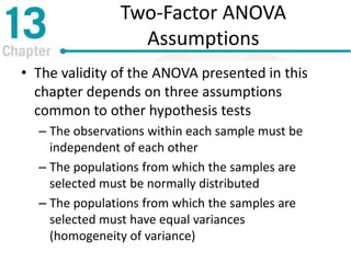
Chapter 13 discusses repeated-measures and two-factor analysis of variance in statistics, highlighting learning outcomes such as understanding ANOVA designs and calculating various statistical measures. It explains the methodology for repeated-measures ANOVA, including its hypotheses, structure, and the benefits of controlling for individual differences among participants. Additionally, it presents the two-factor ANOVA approach, emphasizing main effects, interactions, and the importance of testing assumptions for valid statistical conclusions.
![Learning Check
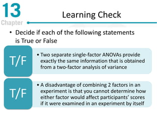
• Decide if each of the following statements
is True or False
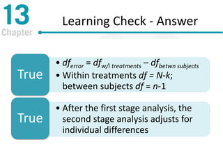
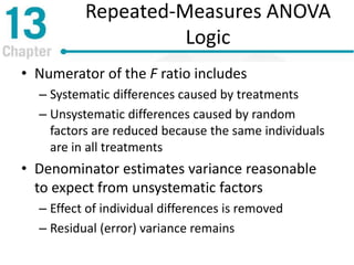
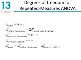
• For the repeated-measures ANOVA,
degrees of freedom for SSerror could be
written as [(N–k) – (n–1)]
T/F
• The first stage of the repeated-
measures ANOVA is the same as the
independent-measures ANOVA
T/F](https://image.slidesharecdn.com/gwe8ch13-150321021037-conversion-gate01/85/Repeated-Measures-and-Two-Factor-Analysis-of-Variance-26-320.jpg)