Downloaded 2,311 times
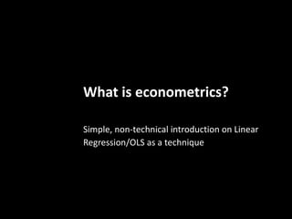


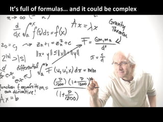

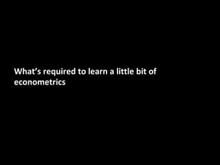


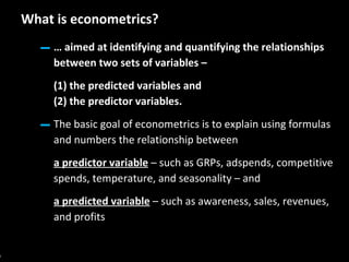
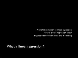

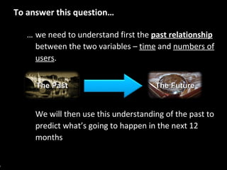

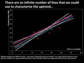

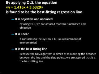

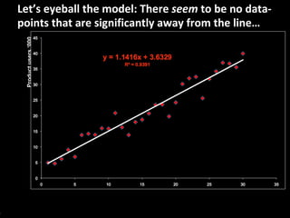
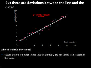

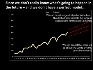
![Let’s now project what’s going to happen in the next 12 months… Time t, in months Product users ‘000 At the end of the next 12 months [by month 42], we can expect to have 543’000 users – if all things remain equal](https://image.slidesharecdn.com/econ101-110501195141-phpapp02/85/Simple-and-Simplistic-Introduction-to-Econometrics-and-Linear-Regression-53-320.jpg)


![This presentation Author: Philip Tiongson [email_address] Audiences: Staff interested in the basics of econometrics](https://image.slidesharecdn.com/econ101-110501195141-phpapp02/85/Simple-and-Simplistic-Introduction-to-Econometrics-and-Linear-Regression-61-320.jpg)


This document serves as a non-technical introduction to econometrics, focusing on linear regression and its application in understanding relationships between predicted and predictor variables. It aims to make econometric concepts accessible to readers with no prior knowledge, emphasizing the importance of a curious mindset and basic arithmetic skills. Additionally, it discusses the use of Ordinary Least Squares (OLS) in deriving a regression line that minimizes distance from actual data points, providing a framework for estimating future trends based on historical data.