Downloaded 1,016 times


The document discusses multicollinearity in regression analysis. It defines multicollinearity as a statistical phenomenon where two or more predictor variables are highly correlated. The presence of multicollinearity can cause problems with estimating coefficients and interpreting results. The document outlines symptoms of multicollinearity, causes, consequences, detection methods, and remedial measures to address multicollinearity issues.
Presentation team members are introduced, focusing on multicollinearity.
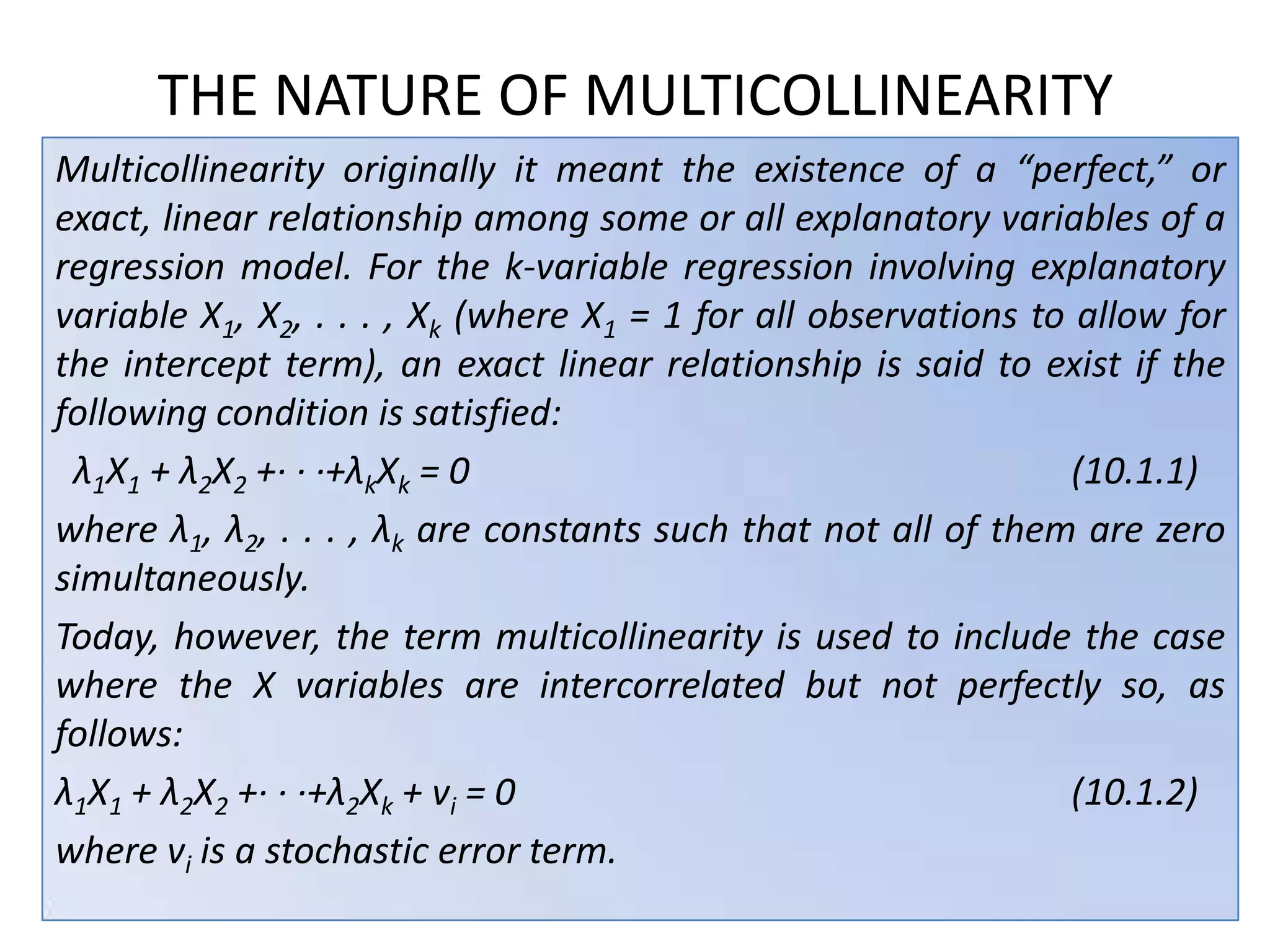
Definition of multicollinearity as high correlation among independent variables in regression.
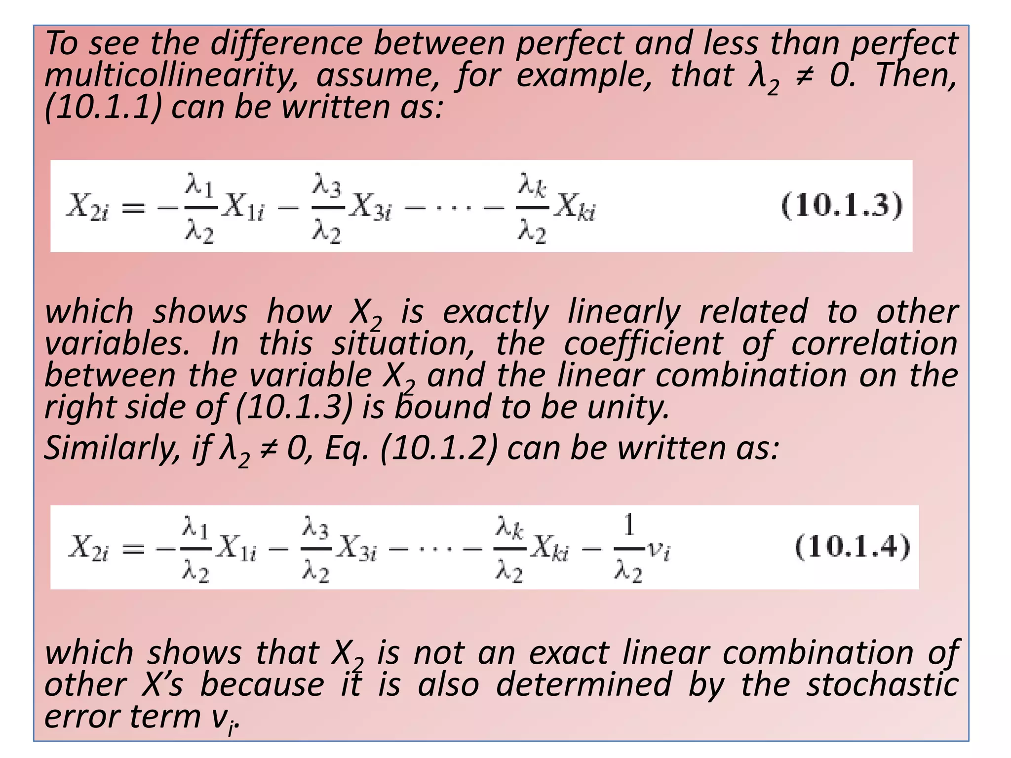
Explains perfect and less-than-perfect multicollinearity and their conditions in regression models.
Defines perfect multicollinearity as identical linear relationships among independent variables.
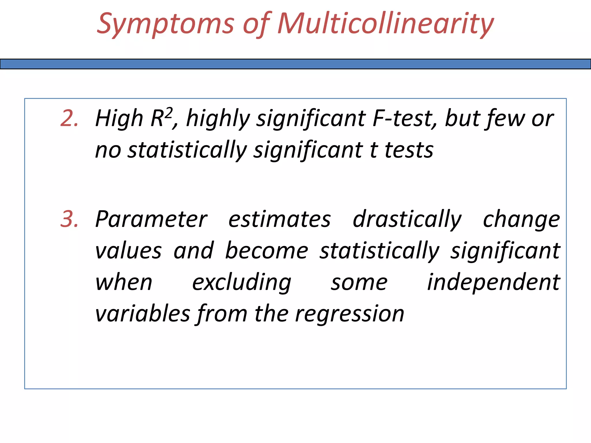
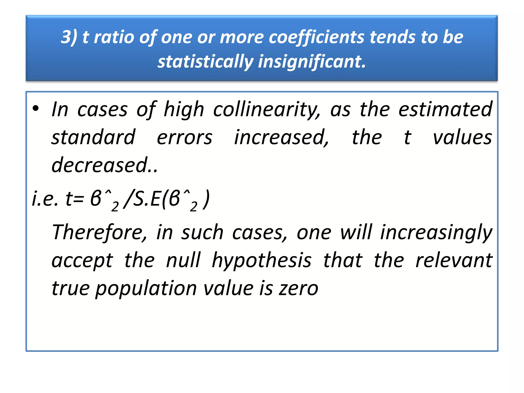
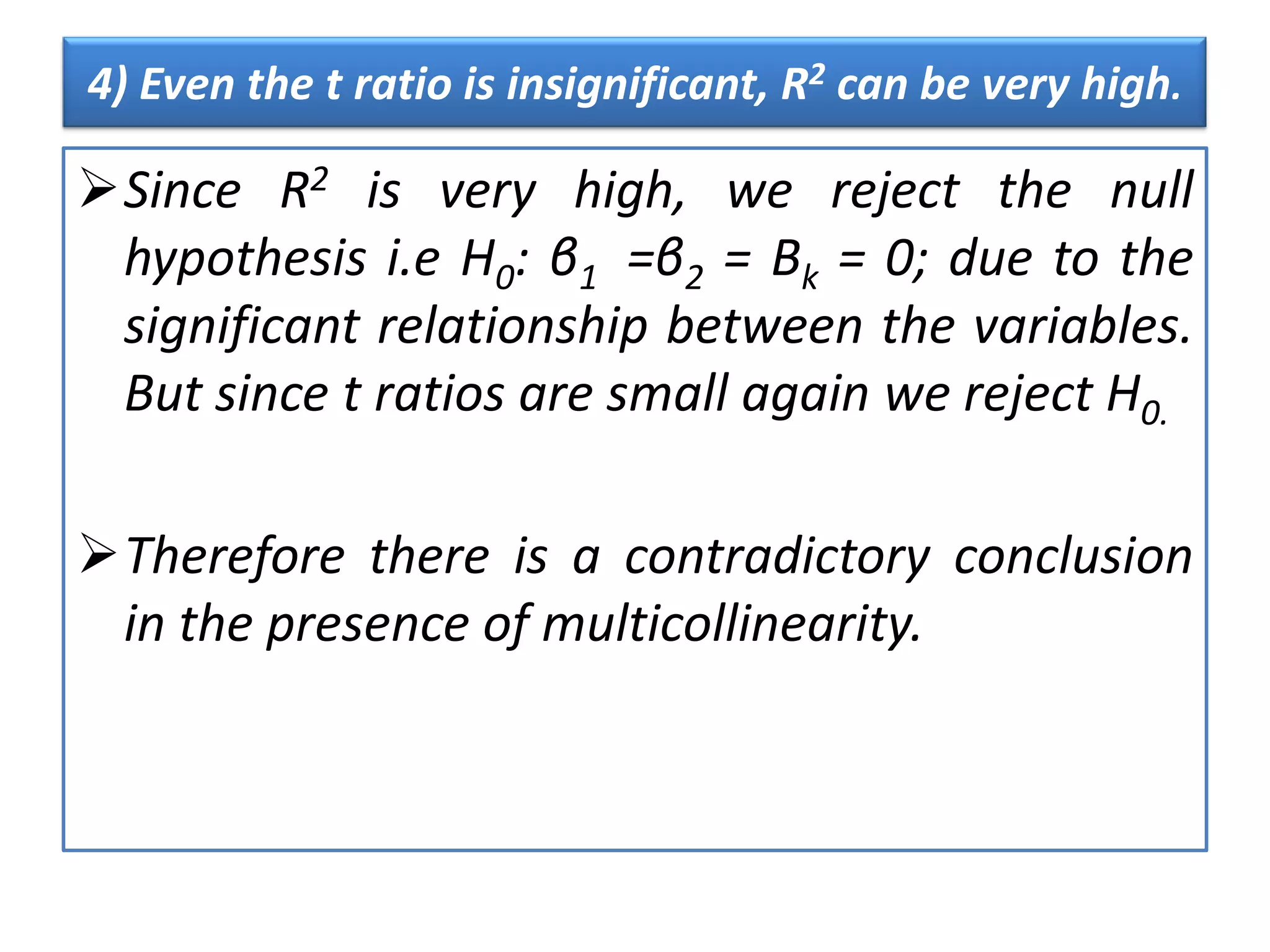
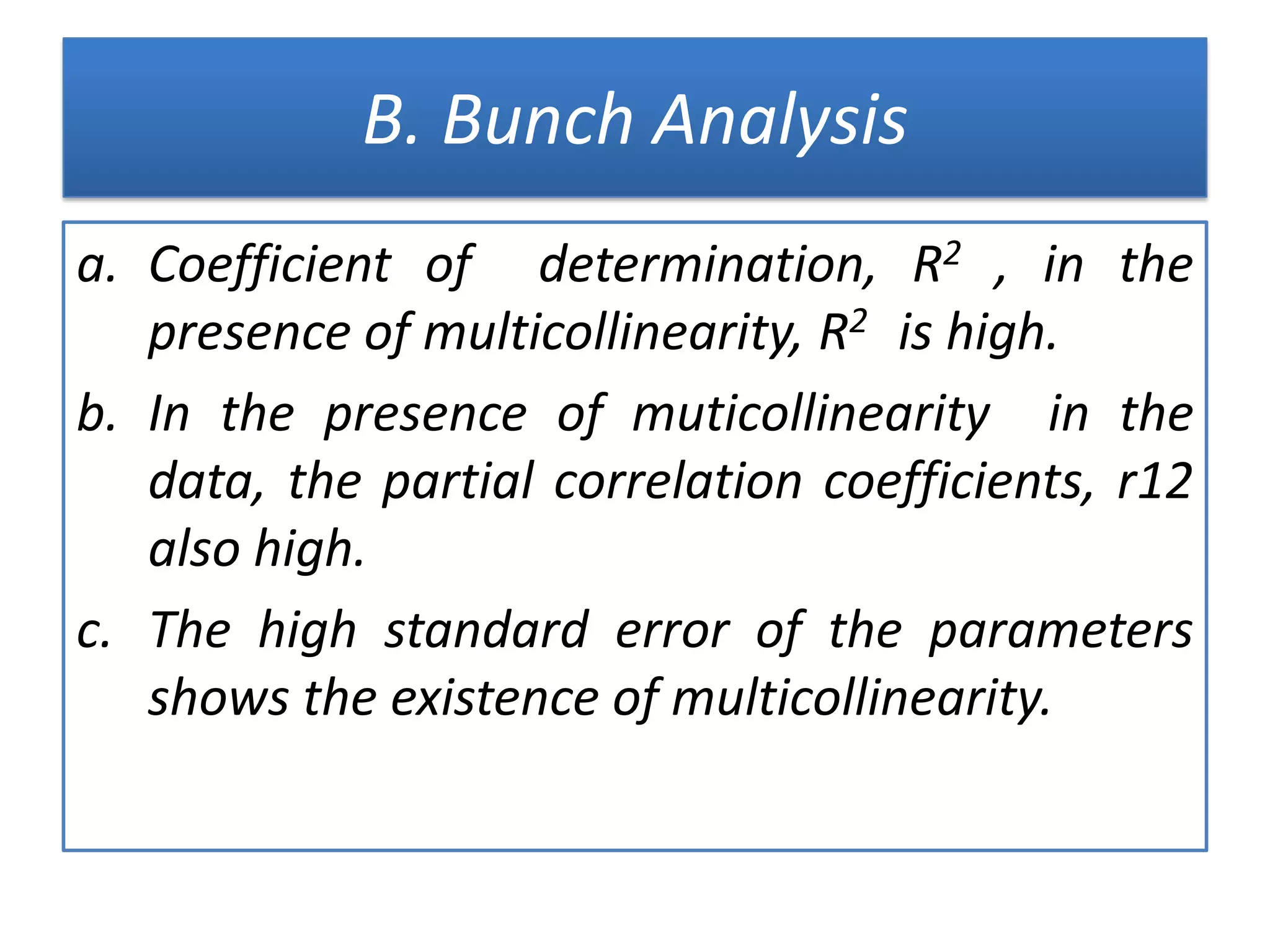
Discusses symptoms like lack of statistical significance of critical variables, high R2 with insignificant t-tests.
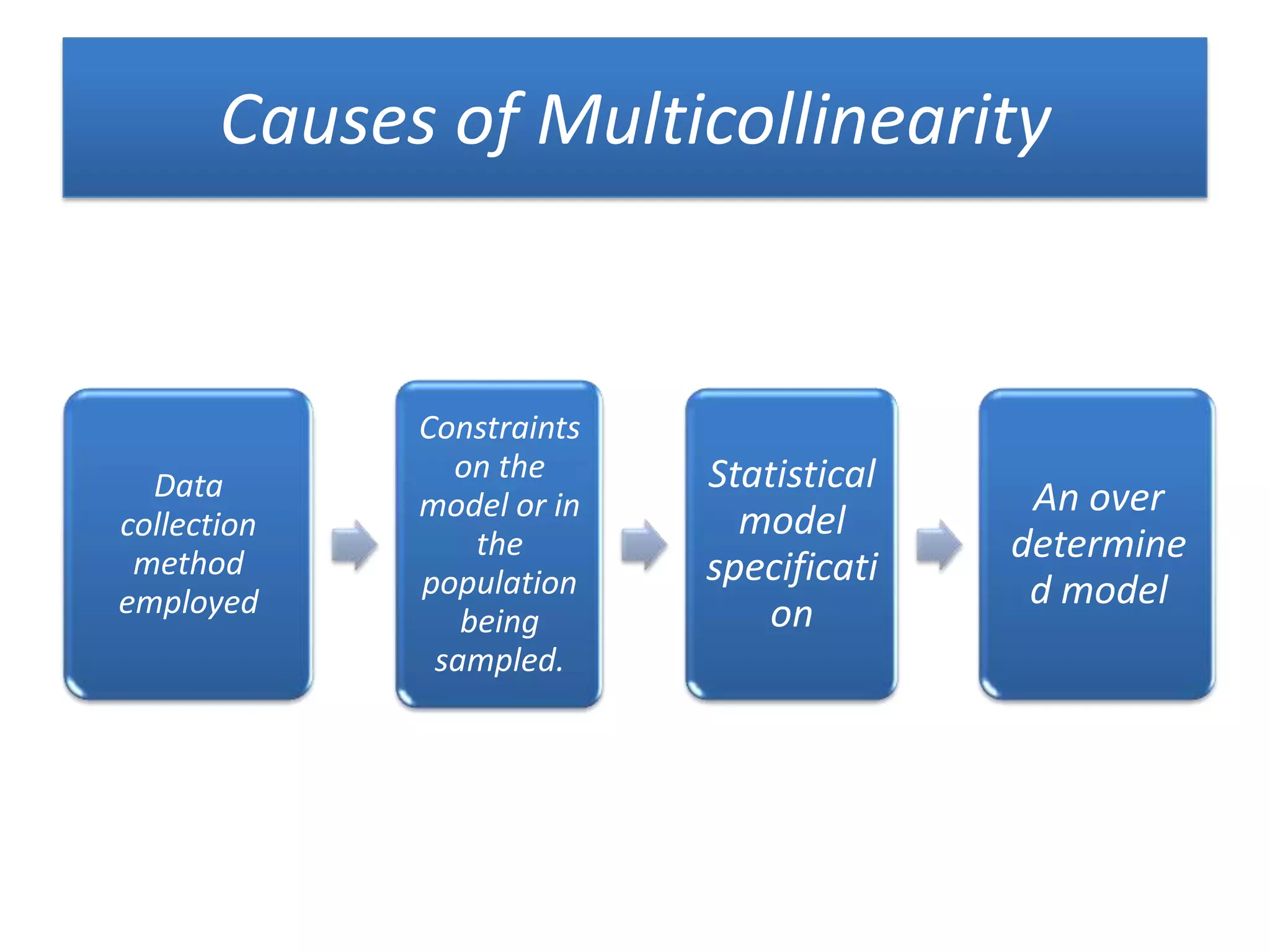
Lists causes including data collection methods and model constraints.
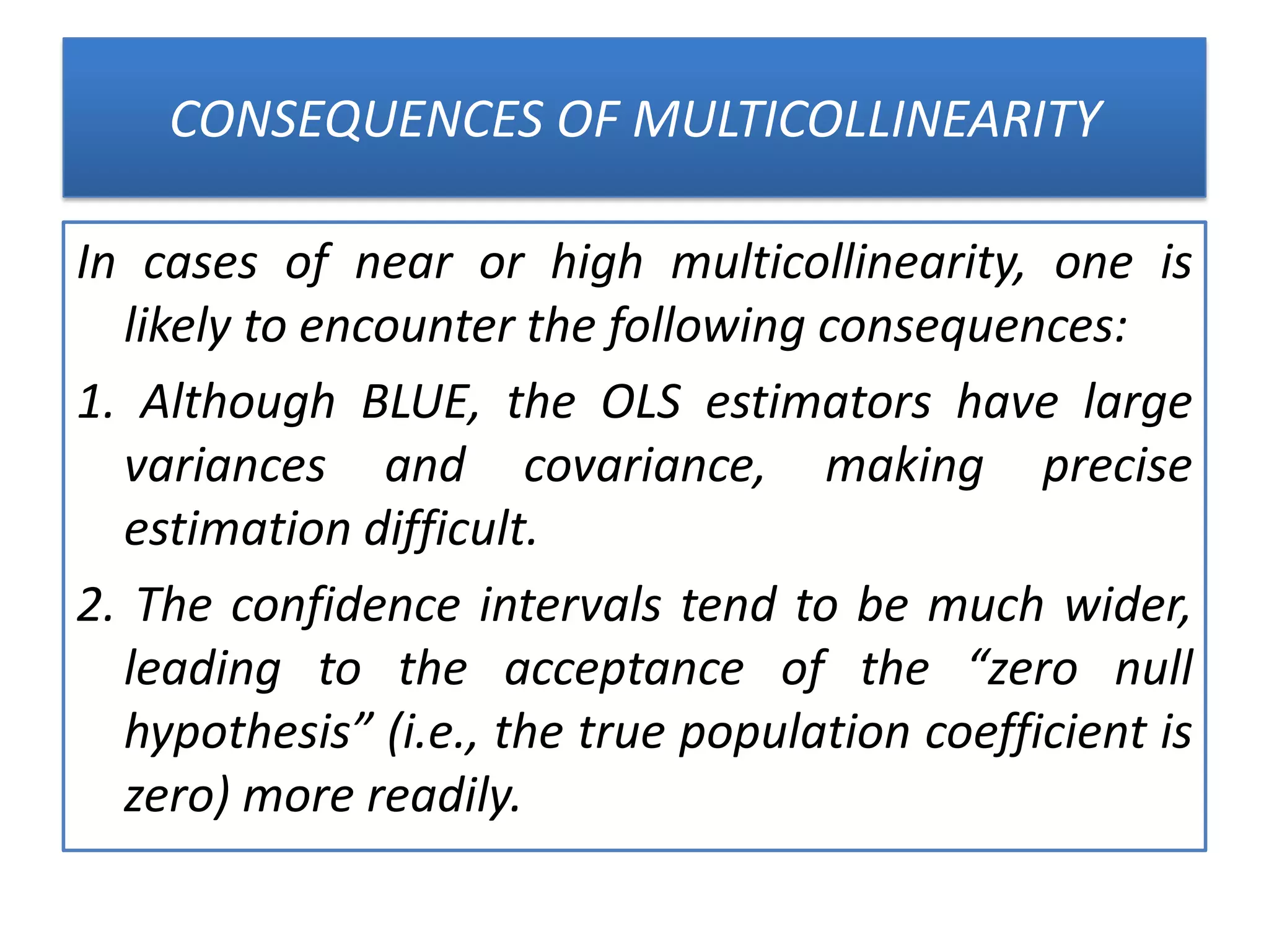
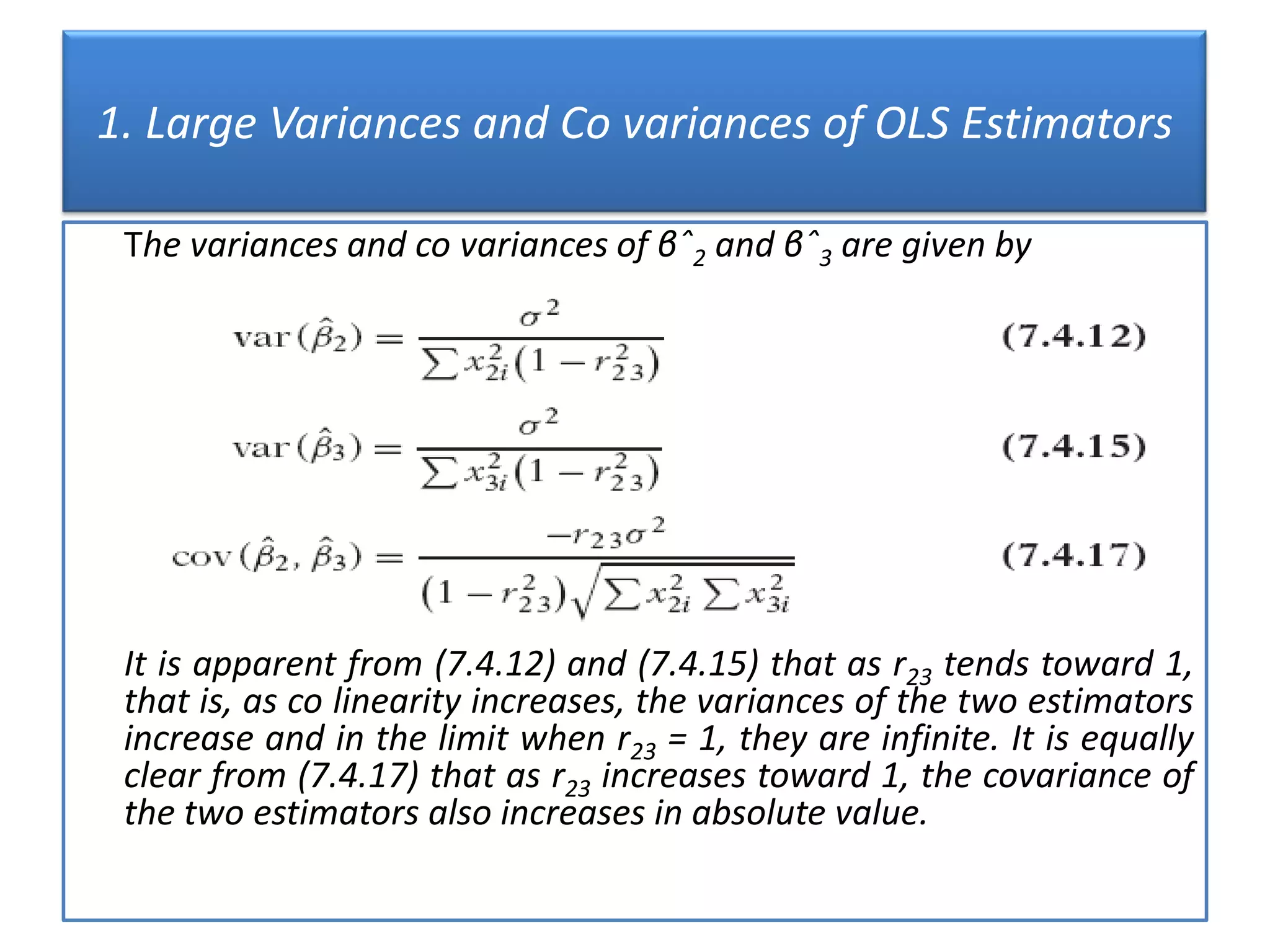
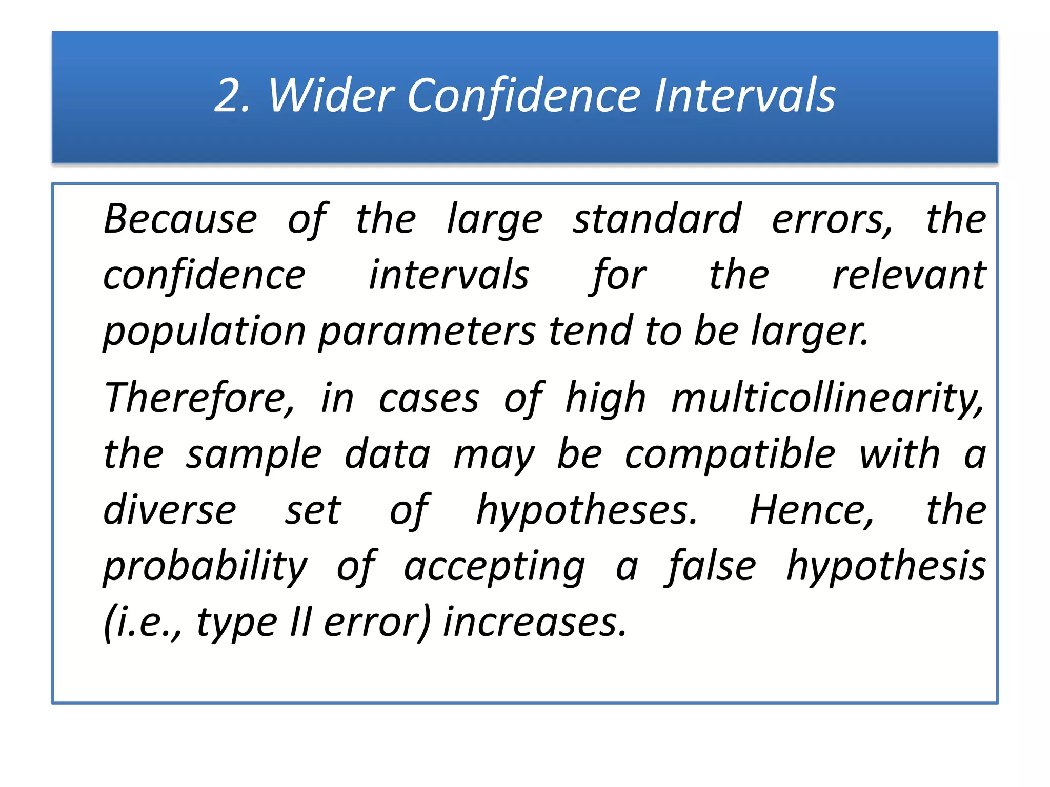
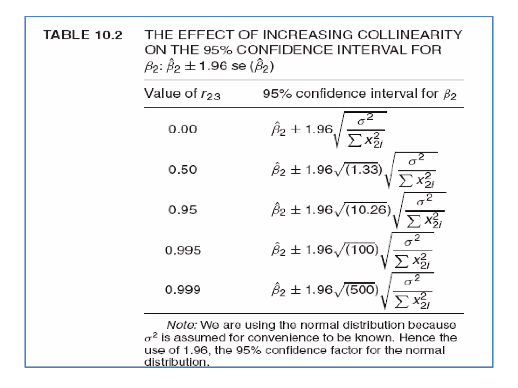
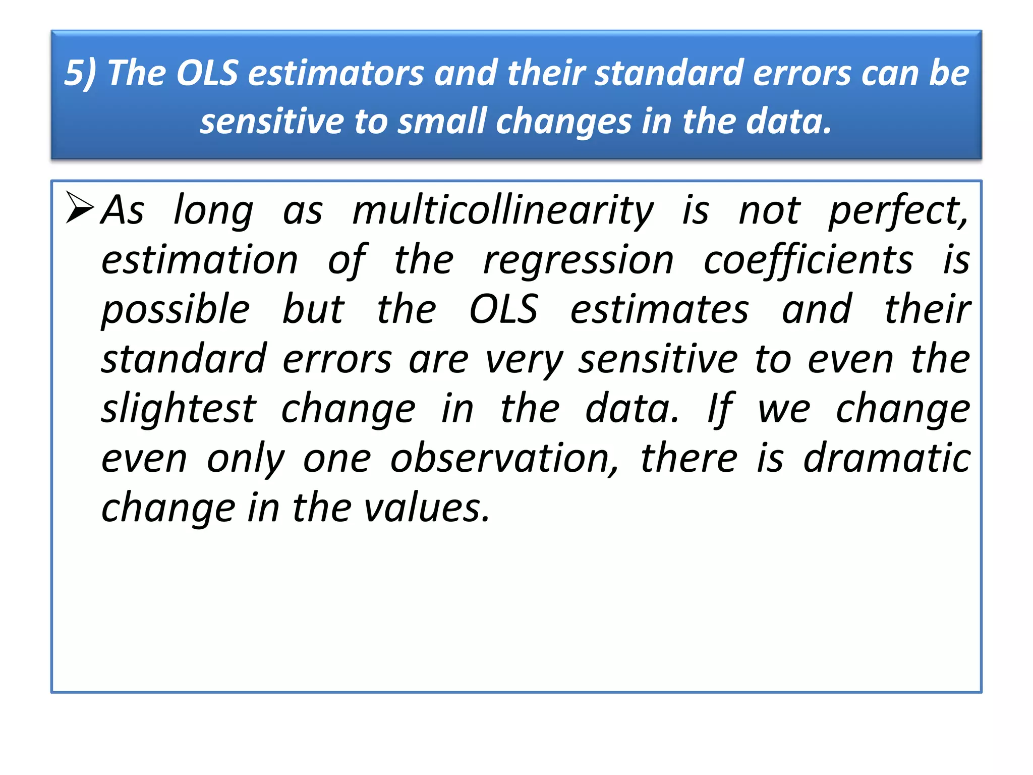
Outlines effects such as large variances of OLS estimators and wider confidence intervals.
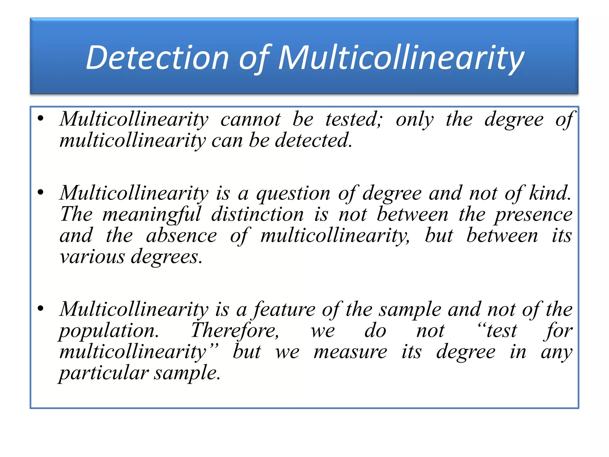
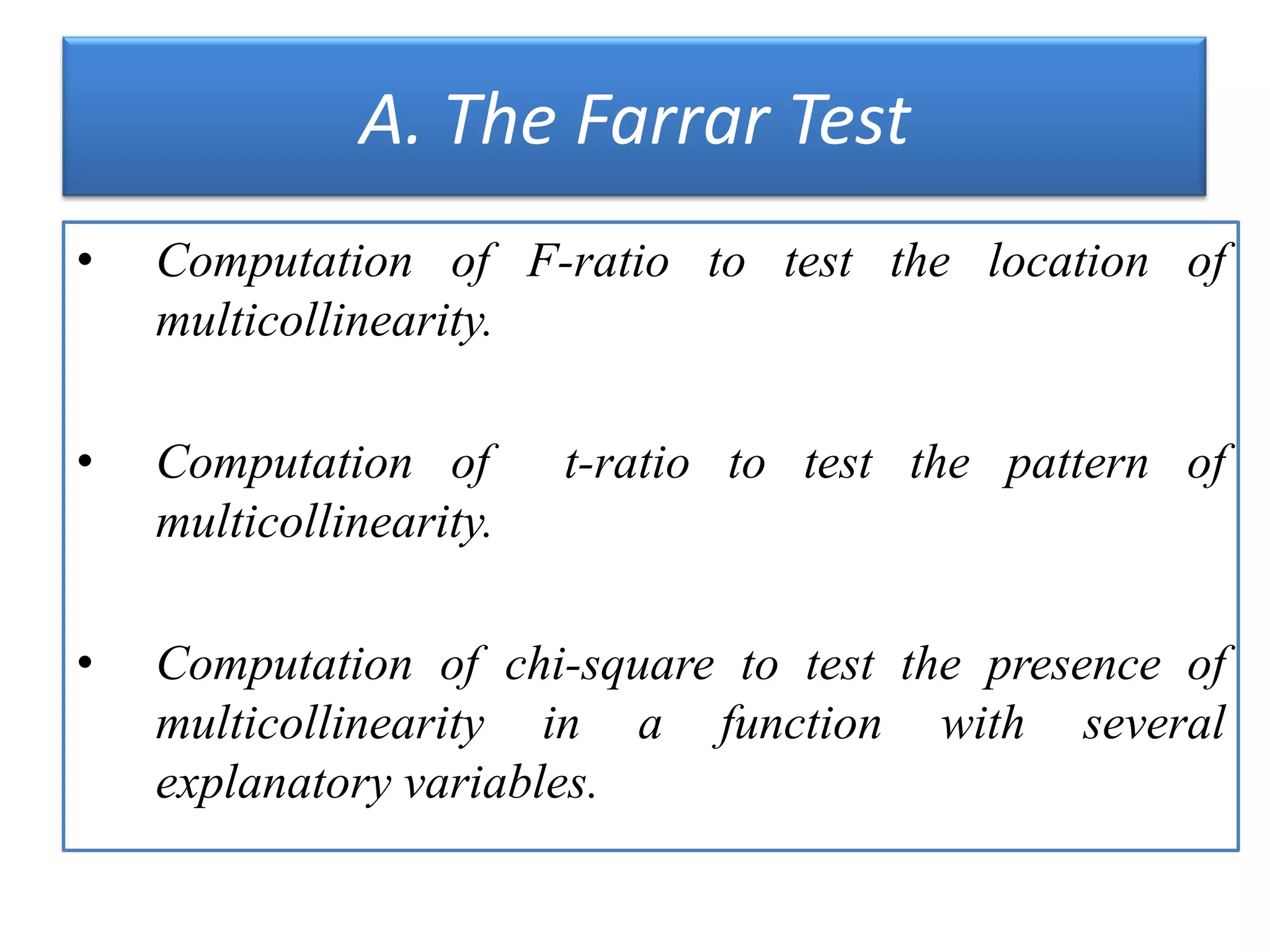
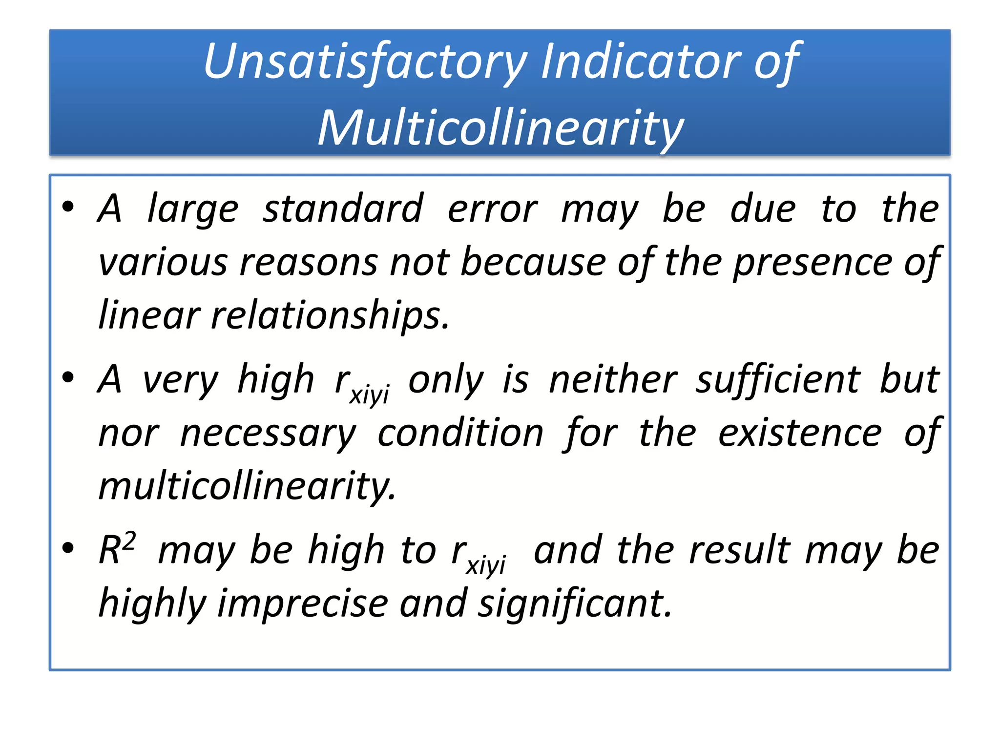
Describes detection methods and limitations, emphasizing the measurement of its degree.
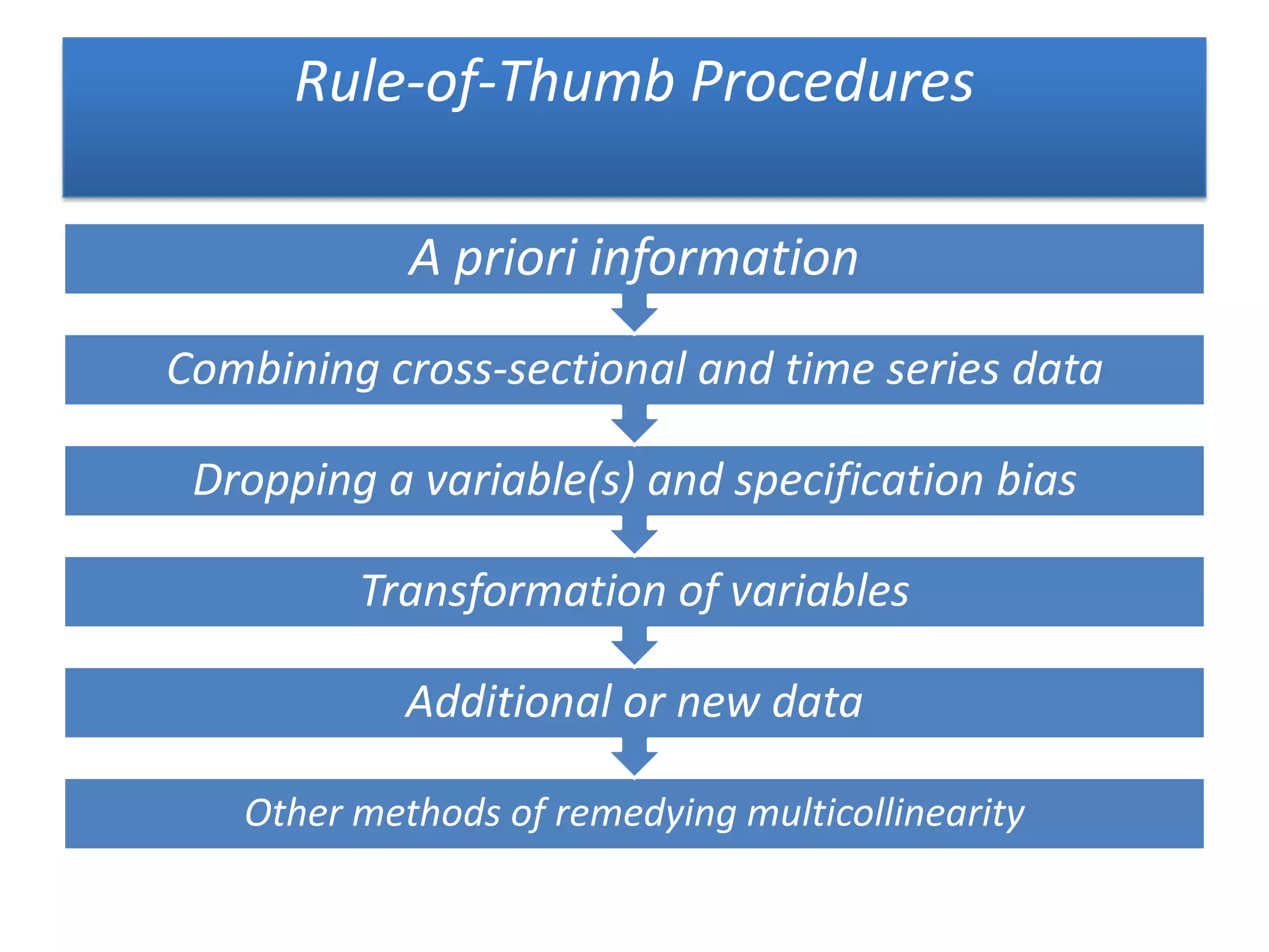
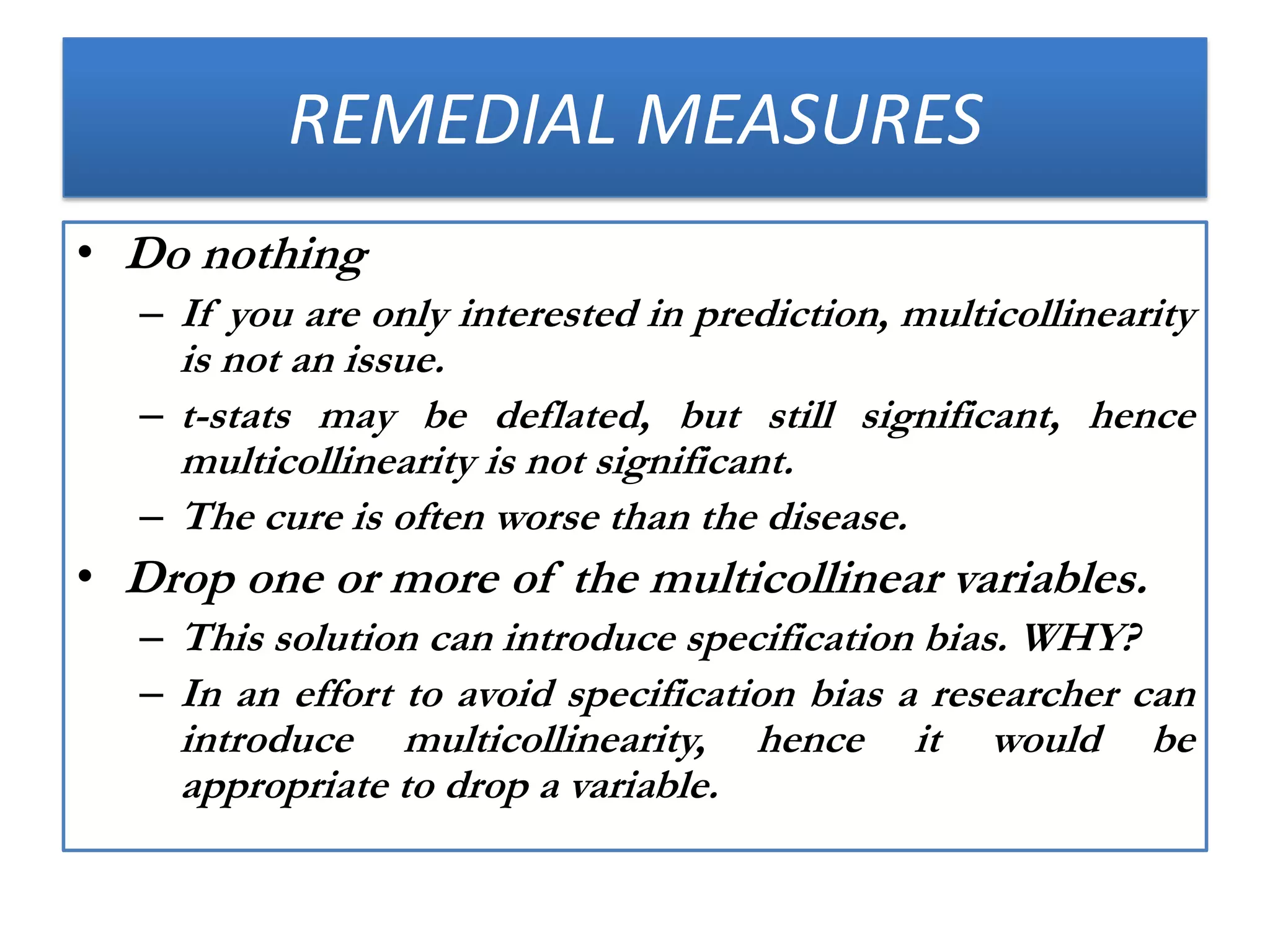
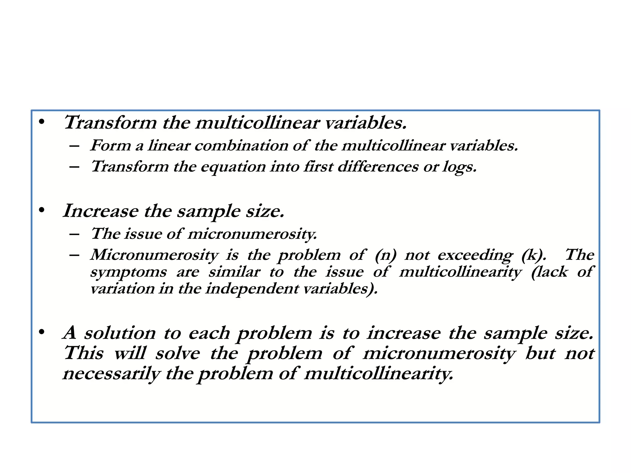
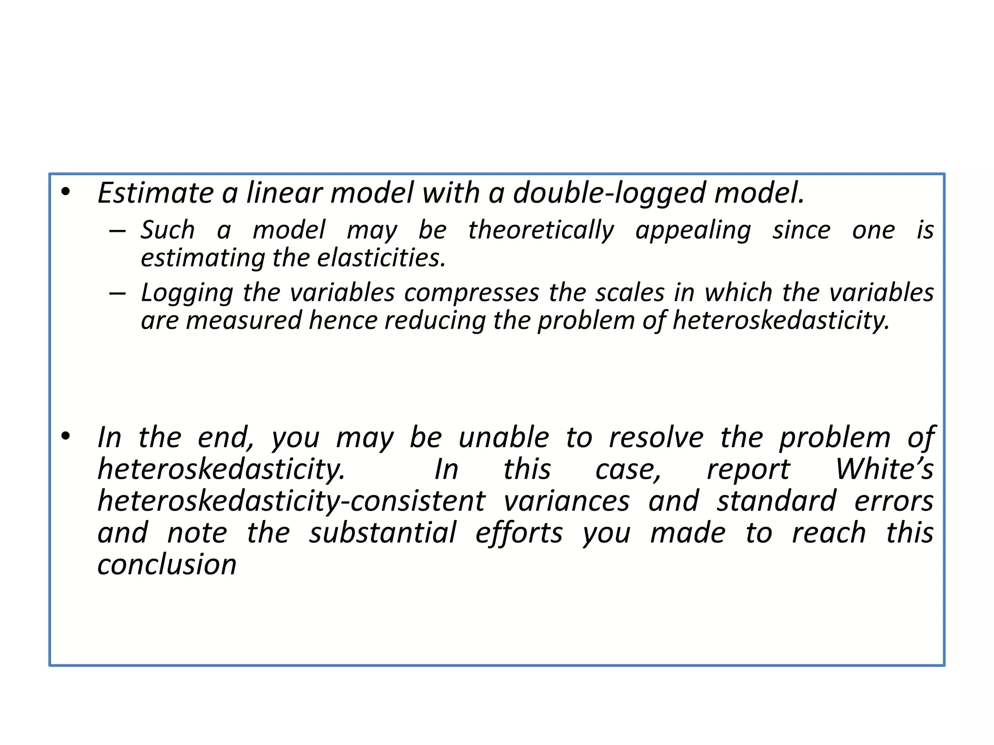
Presents solutions like data transformation and increasing sample size to address multicollinearity.
Summarizes the importance of recognizing and addressing multicollinearity in regression analysis.