RM-10 Hypothesis testing.ppt

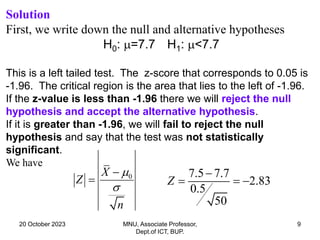
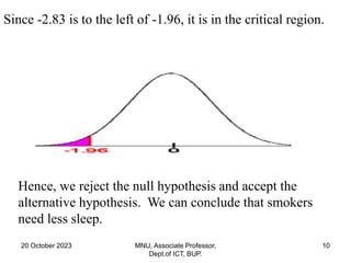
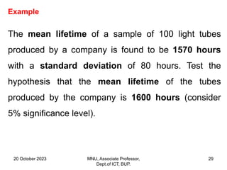
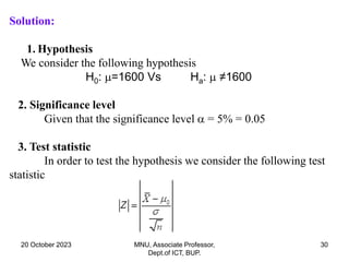
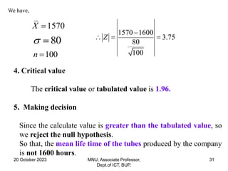
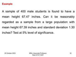
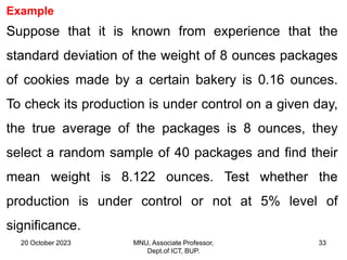
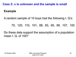
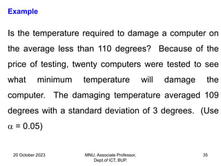
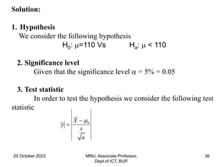
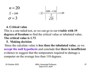
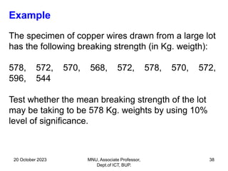
Welcome
to the presentation
on
Hypothesis Testing
Presented by
Dr. Mohammed Nasir Uddin
Associate Professor
Department of ICT,
FST, BUP.

20 October 2023 MNU, Associate Professor,
Dept.of ICT, BUP.
2
TOPICS
Hypothesis
Classification
One & Two tailed Test
Applications

Dept.of ICT, BUP.
3
Hypothesis
An assumption we make about a population
parameter. A statistical hypothesis test is a method
of making statistical decisions using experimental data.
Test of significance or test of a hypothesis
A significance test or test of a hypothesis is a
statistical procedure for reaching a decision.

Dept.of ICT, BUP.
4
Null hypothesis
The statistical hypothesis which is picked up for the
test is known as the null hypothesis. The null
hypothesis is usually denoted by H0.
Example
Let us consider a normal distribution with mean 
and variance 2. Then the hypothesis that the normal
distribution has a specified mean 270 i. e., =5 is
known as the null hypothesis.

Dept.of ICT, BUP.
5
Example
Let us consider a normal distribution with mean  and
variance 2. We are going to test the hypothesis,
H0: =5
Then the alternative hypothesis may be Ha or H1.
Ha:   5
or, Ha:   5
or, Ha:   5
Alternative hypothesis:
Any hypothesis other than the null hypothesis is known as
the alternative hypothesis.
It is usually denoted by Ha or H1.

Dept.of ICT, BUP.
6
The null and alternative hypotheses offer competing answers
to your research question. When the research question asks
“Does the independent variable affect the dependent
variable?”:
•The null hypothesis (H0) answers “No, there’s no effect in
the population.”
•The alternative hypothesis (Ha) answers “Yes, there is an
effect in the population.”
The null and alternative are always claims about the
population.
That’s because the goal of hypothesis testing is to
make inferences about a population based on a sample

Dept.of ICT, BUP.
7
Rejection Regions
Suppose that  = 0.05. We can draw the appropriate
picture and find the Z score for -0.025 and 0.025 . We
call the outside regions the rejection regions.
We call the blue areas the rejection region since if
the value of Z falls in these regions, we can say that
the null hypothesis is very unlikely so we can reject
the null hypothesis.

Dept.of ICT, BUP.
8
Example
50 smokers were questioned about the number of hours they
sleep each day. We want to test the hypothesis that the
smokers need less sleep than the general public which needs
an average of 7.7 hours of sleep. We follow the steps below:
a. Compute a rejection region for a significance level of
0.05.
b. If the sample mean is 7.5 and the standard deviation is 0.5,
what can you conclude?

Dept.of ICT, BUP.
9
Solution
First, we write down the null and alternative hypotheses
H0: =7.7 H1: <7.7
This is a left tailed test. The z-score that corresponds to 0.05 is
-1.96. The critical region is the area that lies to the left of -1.96.
If the z-value is less than -1.96 there we will reject the null
hypothesis and accept the alternative hypothesis.
If it is greater than -1.96, we will fail to reject the null
hypothesis and say that the test was not statistically
significant.
We have
7.5 7.7
2.83
0.5
50
Z

  
0
X
Z
n





Dept.of ICT, BUP.
10
Hence, we reject the null hypothesis and accept the
alternative hypothesis. We can conclude that smokers
need less sleep.
Since -2.83 is to the left of -1.96, it is in the critical region.

Dept.of ICT, BUP.
11
Test
A body of rules which leads to the decision regarding
acceptance or rejection of the hypothesis is called a test. The
statistic which is usually used to test the parameter of a
population is known as the test statistic.
The test may be classified as
One-tailed test
Two-tailed test

Dept.of ICT, BUP.
12
One-tailed test
A test for which the entire rejection region lies in only
two tails either in the right tail or in the left tail of the
sampling distribution of the test statistic is called one-
tailed.
If we are interested to test the hypothesis
H0:  = 0 vs Ha:   0 then we should use a right-
tailed test.
If we test H0:  = 0 vs Ha:   0 then we should use
the left tailed test.

Dept.of ICT, BUP.
13
.
Fig: Sampling Distribution of the Statistic z, Right
and Left-Tailed Test, 0.05 Level of Significance.

Dept.of ICT, BUP.
14
Two-tailed test
A test for which the rejection region is divided equally
between two tails of the sampling distributions of
the test statistics is called a two-tailed test. If we are
interested to test the
H0:  = 0 vs Ha:   0 then we should use two-tailed
test.
Fig: Regions of Non-rejection and Rejection for a Two-Tailed Test, 0.05
Level of Significance.

Dept.of ICT, BUP.
15
Critical value
The value of the standard statistic ( Z or t ) is beyond
which we reject the null hypothesis.
The boundary between the acceptance and rejection
regions.
Error
When using probability to decide whether a statistical
test provides evidence for or against our predictions,
there is always a chance of driving the wrong conclusions.
Even when choosing a probability level of 95%, there is
always a 5% chance that one rejects the null hypothesis
when it was actually correct. This is called Type I error,
represented by the Greek letter, . The probability of a
type I error () is called the significance level.

Dept.of ICT, BUP.
16
It is possible to an error in the opposite way if one
fails to reject the null hypothesis when it is, in fact,
incorrect. This is called Type II error, represented by
the Greek letter . These two errors are represented
in the following chart.
.
Table: Types of error
Type of decision H0 true H0 false
Reject H0 Type I error ( ) Correct decision (1-)
Accept H0 Correct decision (1- ) Type II error ()

Dept.of ICT, BUP.
17
A related concept is a power, which is the probability of
rejecting the null hypothesis when it is actually false.
Power is simply 1 minus the Type II error rate and is
usually expressed as (1-).
When choosing the probability level of a test, it is possible
to control the risk of committing a Type I error by
choosing an appropriate .

Dept.of ICT, BUP.
18
P-values
There is another way to interpret the test statistic. In hypothesis
testing, we make a yes or no decision without discussing
borderline cases.
For example, with  = 0.06, a two-tailed test will indicate
rejection of H0 for a test statistic of Z= 2 or for Z = 6, but Z = 6 is
much stronger evidence than Z = 2 . To show this difference we
write the p-value which is the lowest significance level such that
we will still reject Ho.
For a two-tailed test, we use twice the table value to find p, and
for a one-tailed test, we use the table value.

Dept.of ICT, BUP.
19
Example
Suppose that we want to test the hypothesis with a
significance level of 0.05 that the climate has
changed since industrialization. Suppose that the
mean temperature throughout history is 50
degrees. During the last 40 years, the mean
temperature has been 51 degrees with a standard
deviation of 2 degrees. What can we conclude?

Dept.of ICT, BUP.
20
Solution:
We have,
H0: =50 H1: ≠ 50
We compute the z score:
The table gives us 0.9992 .
So that
p = (1 - 0.9992)(2) = 0 .002
Since 0.002 < 0.05
We can conclude that there has been a change in
temperature.
Note that small p-values will result in a rejection of H0 and
large p-values will result in failing to reject H0 .

Dept.of ICT, BUP.
21
Steps in Hypothesis Testing
Step 1
Identify the null hypothesis H0 and the alternate hypothesis HA .
Step 2
Choose . The value should be small, usually less than 10%. It
is important to consider the consequences of both types of
errors.
Step 3
Select the test statistic and determine its value from the sample
data. This value is called the observed value of the test
statistic. Remember that a t statistic is usually appropriate for a
small number of samples; for larger number of samples, a z
statistic can work well if data are normally distributed.

Dept.of ICT, BUP.
22
Step 4
Compare the observed value of the statistic to the critical
value obtained for the chosen .
Step 5
Make a decision.
If the test statistic falls in the critical region: Reject H0 in favor of
HA .
If the test statistic does not fall in the critical region: Conclude
that there is not enough evidence to reject H0.

Dept.of ICT, BUP.
23
Important tests of significance
The important tests of significance in statistics can
be classified broadly as
i. Normal test
ii. t test
iii. 2 Test
iv.F test

Dept.of ICT, BUP.
24
Test of significance about mean
Here we consider the following cases:
 Comparison of a sample mean with an
assigned population mean.
Comparison of two independent sample means.
Comparison of two correlated sample means.
Comparison of k (k>2) independent sample
means.

Dept.of ICT, BUP.
25
Comparison of a sample mean with an assigned
population mean
Case 1:  is known or estimated from a large sample.
Case 2:  is unknown and the sample is small.

Dept.of ICT, BUP.
26
Case – 1 ( is known or
large sample)
Case – 2 ( is unknown
or small sample)
Hypothesis
H0 :  = 0
HA :   0
Hypothesis
H0 :  = 0
HA :   0
Test Statistic Test Statistic
0
X
Z
n




0
X
t
s
n


 With n-1 d.f.
Where, 1
X x
n
 
 
2 2 2
1
1
s x nx
n
 

 

Dept.of ICT, BUP.
27
How do you find the critical value of Z?
1. Divide the significance level α by 2.
2. 1 - α/2 = 1 – 0.01= 0.99.
3. Search the value 0.99 in the z table given below.
4. 2.3 + 0.03 = 2.33.

Dept.of ICT, BUP.
28
Common confidence levels and their critical
values (CV)
Confidence Level Two Sided CV One Sided CV
90% 1.64 1.28
95% 1.96 1.65
99% 2.58 2.33

Dept.of ICT, BUP.
29
Example
The mean lifetime of a sample of 100 light tubes
produced by a company is found to be 1570 hours
with a standard deviation of 80 hours. Test the
hypothesis that the mean lifetime of the tubes
produced by the company is 1600 hours (consider
5% significance level).

Dept.of ICT, BUP.
30
Solution:
1. Hypothesis
We consider the following hypothesis
H0: =1600 Vs Ha:  ≠1600
2. Significance level
Given that the significance level  = 5% = 0.05
3. Test statistic
In order to test the hypothesis we consider the following test
statistic

Dept.of ICT, BUP.
31
We have,
1570
X 
80
 
100
n 
1570 1600
3.75
80
100
Z

  
4. Critical value
The critical value or tabulated value is 1.96.
5. Making decision
Since the calculate value is greater than the tabulated value, so
we reject the null hypothesis.
So that, the mean life time of the tubes produced by the company
is not 1600 hours.

Dept.of ICT, BUP.
32
Example
A sample of 400 male students is found to have a
mean height 67.47 inches. Can it be reasonably
regarded as a sample from a large population with
mean height 67.39 inches and standard deviation 1.30
inches? Test at 5% level of significance.

Dept.of ICT, BUP.
33
Example
Suppose that it is known from experience that the
standard deviation of the weight of 8 ounces packages
of cookies made by a certain bakery is 0.16 ounces.
To check its production is under control on a given day,
the true average of the packages is 8 ounces, they
select a random sample of 40 packages and find their
mean weight is 8.122 ounces. Test whether the
production is under control or not at 5% level of
significance.

Dept.of ICT, BUP.
34
Case 2:  is unknown and the sample is small
Example
A random sample of 10 boys had the following I. Q’s:
70, 120, 110, 101, 88, 83, 95, 98, 107, 100
Do these data support the assumption of a population
mean I. Q. of 100?

Dept.of ICT, BUP.
35
Example
Is the temperature required to damage a computer on
the average less than 110 degrees? Because of the
price of testing, twenty computers were tested to see
what minimum temperature will damage the
computer. The damaging temperature averaged 109
degrees with a standard deviation of 3 degrees. (Use
 = 0.05)

Dept.of ICT, BUP.
36
Solution:
1. Hypothesis
We consider the following hypothesis
H0: =110 Vs Ha:  < 110
2. Significance level
Given that the significance level  = 5% = 0.05
3. Test statistic
In order to test the hypothesis we consider the following test
statistic
0
X
t
s
n




Dept.of ICT, BUP.
37
20
n 
109
X 
3
 
109 110
1.49
3
20
t

  
4. Critical value
This is a one tailed test, so we can go to our t-table with 19
degrees of freedom to find the critical value or tabulated value.
The critical value is 1.73.
5. Making decision
Since the calculate value is less than the tabulated value, so we
accept the null hypothesis and conclude that there is insufficient
evidence to suggest that the temperature required to damage a
computer on the average less than 110 degrees.

Dept.of ICT, BUP.
38
Example
The specimen of copper wires drawn from a large lot
has the following breaking strength (in Kg. weigth):
578, 572, 570, 568, 572, 578, 570, 572,
596, 544
Test whether the mean breaking strength of the lot
may be taking to be 578 Kg. weights by using 10%
level of significance.

Dept.of ICT, BUP.
40
THANKS
FOR
PATIENCE HEARING

RM-10 Hypothesis testing.ppt

More Related Content

Similar to RM-10 Hypothesis testing.ppt

Recently uploaded

RM-10 Hypothesis testing.ppt