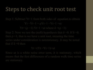
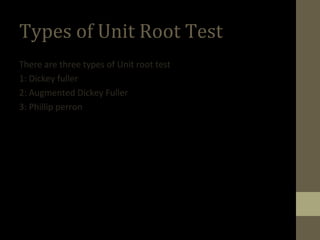
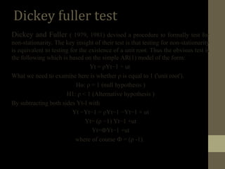
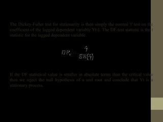
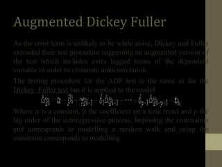
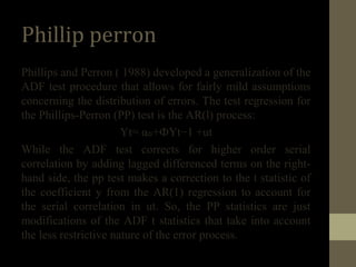
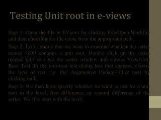
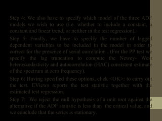
The document provides an overview of unit root tests in time series analysis, explaining the concept of a unit root, how to check for it, and detailing three types of tests: Dickey-Fuller, Augmented Dickey-Fuller, and Phillips-Perron. It outlines the procedure to test for non-stationarity in autoregressive models and offers a step-by-step guide on conducting unit root tests using E-Views software. The referenced materials suggest further reading in applied and basic econometrics.

2. Govt. college for Women
University
Madina town, Fsd

3. Unit Root Test

4. Contents
1: What is unit root?
2: How to check unit root?
3: Types of unit root test
4: Dickey fuller
5: Augmented dickey fuller
6: Phillip perron
7: Testing Unit Root on E-views

5. Unit Root Test
What is unit root?
A unit root test is a statistical test for the proposition that in
a autoregressive statistical model of a time series, the
autoregressive parameter is one. A unit root is an attribute of
a statistical model of a time series whose autoregressive
parameter is one. It is as:
yt=ρyt-1+ut
where -1≤ρ≤1
If ρ is in fact 1, we face what is known as the unit root
problem that is a situation of non stationary .

6. How to check Unit Root?
We start with Yt = ρYt−1 +ut
−1≤ ρ ≤1
where ut is a white noise error term. We know that if ρ
=1, that is the case of the unit root, which we know is a
non-stationary stochastic process. Then we simply
regress Yt on its lagged value Yt−1 and find out if the
estimated ρ is statistically equal to 1? If it is, then Yt is
nonstationary. This is the general idea behind the unit
root test of stationarity.

7. Steps to check unit root test
Step 1: Subtract Yt−1 from both sides of equation.to obtain
Yt −Yt−1 = ρYt−1 −Yt−1 +ut
Yt= (ρ −1) Yt−1 +ut where δ =(ρ −1)
Step 2: Now we test the (null) hypothesis that δ =0. If δ =0,
then ρ =1, that is we have a unit root, meaning the time
series under consideration is nonstationary. It may be noted
that if δ =0 then
Yt =(Yt −Yt−1)=ut
Since ut is a white noise error term, it is stationary, which
means that the first differences of a random walk time series
are stationary.

8. Types of Unit Root Test
There are three types of Unit root test
1: Dickey fuller
2: Augmented Dickey Fuller
3: Phillip perron

9. Dickey fuller test
Dickey and Fuller ( 1979, 1981) devised a procedure to formally test for
non-stationarity. The key insight of their test is that testing for non-stationarity
is equivalent to testing for the existence of a unit root. Thus the obvious test is
the following which is based on the simple AR(1) model of the form:
Yt = ρYt−1 + ut
What we need to examine here is whether ρ is equal to 1 ('unit root').
Ho: ρ = 1 (null hypothesis )
H1: ρ < 1 (Alternative hypothesis )
By subtracting both sides Yt-I with
Yt −Yt−1 = ρYt−1 −Yt−1 + ut
Yt= (ρ −1) Yt−1 +ut
Yt=ФYt−1 +ut
where of course Ф = (ρ -1).

10. The Dickey-Fuller test for stationarity is then simply the normal 't' test on the
coefficient of the lagged dependent variable Yt-I. The DF-test statistic is the t
statistic for the lagged dependent variable.
If the DF statistical value is smaller in absolute terms than the critical value
then we reject the null hypothesis of a unit root and conclude that Yt is a
stationary process.

11. Augmented Dickey Fuller
As the error term is unlikely to be white noise, Dickey and Fuller
extended their test procedure suggesting an augmented version of
the test which includes extra lagged terms of the dependent
variable in order to eliminate autocorrelation.
The testing procedure for the ADF test is the same as for the
Dickey–Fuller test but it is applied to the model
Where α is a constant, β the coefficient on a time trend and ρ the
lag order of the autoregressive process. Imposing the constraints
and corresponds to modelling a random walk and using the
constraint corresponds to modelling.

12. Phillip perron
Phillips and Perron ( 1988) developed a generalization of the
ADF test procedure that allows for fairly mild assumptions
concerning the distribution of errors. The test regression for
the Phillips-Perron (PP) test is the AR(l) process:
Yt= αₒ+ФYt−1 +ut
While the ADF test corrects for higher order serial
correlation by adding lagged differenced terms on the right-hand
side, the pp test makes a correction to the t statistic of
the coefficient y from the AR(1) regression to account for
the serial correlation in ut. So, the PP statistics are just
modifications of the ADF t statistics that take into account
the less restrictive nature of the error process.

13. Testing Unit root in e-views
Step 1: Open the file in EViews by clicking File/Open/Workfile
and then choosing the file name from the appropriate path.
Step 2: Let's assume that we want to examine whether the series
named GDP contains a unit root. Double click on the series
named 'gdp' to open the series window and choose View/Unit
Root Test .In the unit-root test dialog box that appears, choose
the type of test (i.e. the' Augmented Dickey-Fuller test) by
clicking on it.
Step 3: We then have specify whether we want to test for a unit
root in the level, first difference, or second difference of the
series. We first start with the level.

14. Step 4: We also have to specify which model of the three ADF
models we wish to use (i.e. whether to include a constant, a
constant and linear trend, or neither in the test regression).
Step 5: Finally, we have to specify the number of lagged
dependent variables to be included in the model in order to
correct for the presence of serial correlation . (For the PP test we
specify the lag truncation to compute the Newey- West
heteroskedasticity and autocorrelation (HAC) consistent estimate
of the spectrum at zero frequency).
Step 6: Having specified these options, click <OK>: to carry out
the test. EViews reports the test statistic together with the
estimated test regression.
Step 7: We reject the null hypothesis of a unit root against the
alternative if the ADF statistic is less than the critical value, and
we conclude that the series is stationary.

15. References
1: Applied Econometrics
(Dimitrios Asterius and stephen)
2: Basic econometrics
(Damodar N. Gujarati)
3:http://economics.about.com/od/economicsglossar
y/g/unitroottest.htm
4: http://en.wikipedia.org/wiki/Phillips%E2%80%93Perron_test.htm