Downloaded 672 times

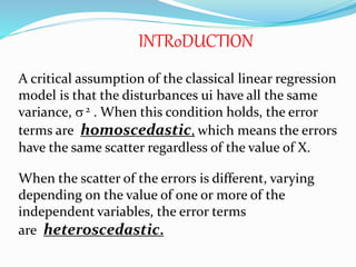
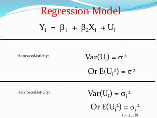
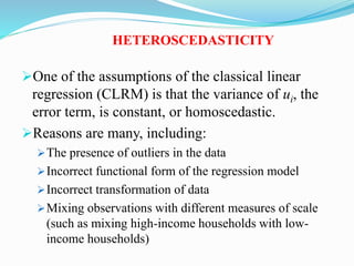
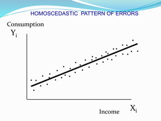
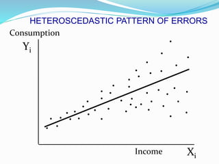
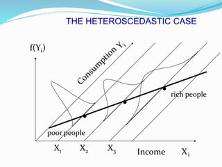
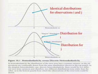
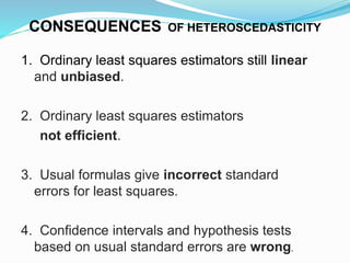
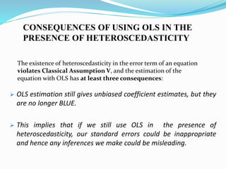
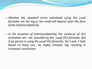
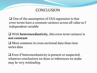


Heteroscedasticity occurs when the variance of the error terms in a regression model are not constant, but instead vary depending on the values of the independent variables. While ordinary least squares estimators remain unbiased, their standard errors may be incorrect under heteroscedasticity. This means that confidence intervals and hypothesis tests based on the usual standard errors are unreliable and can lead to misleading conclusions.