Download as PDF, PPTX


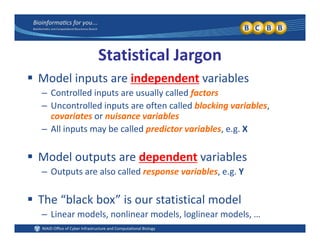
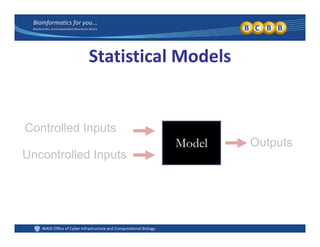


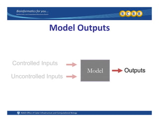


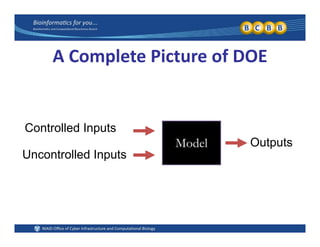


This document provides an overview of design of experiments (DOE). It discusses key concepts like controlled and uncontrolled inputs, response variables, experimental and sampling units, and different types of statistical designs. Specifically, it explains that a designed experiment involves planned statistical considerations to increase efficiency. It also describes completely randomized designs and randomized complete block designs as two basic statistical designs. The goal of DOE is to obtain unbiased and efficient experimental results.