Downloaded 4,024 times
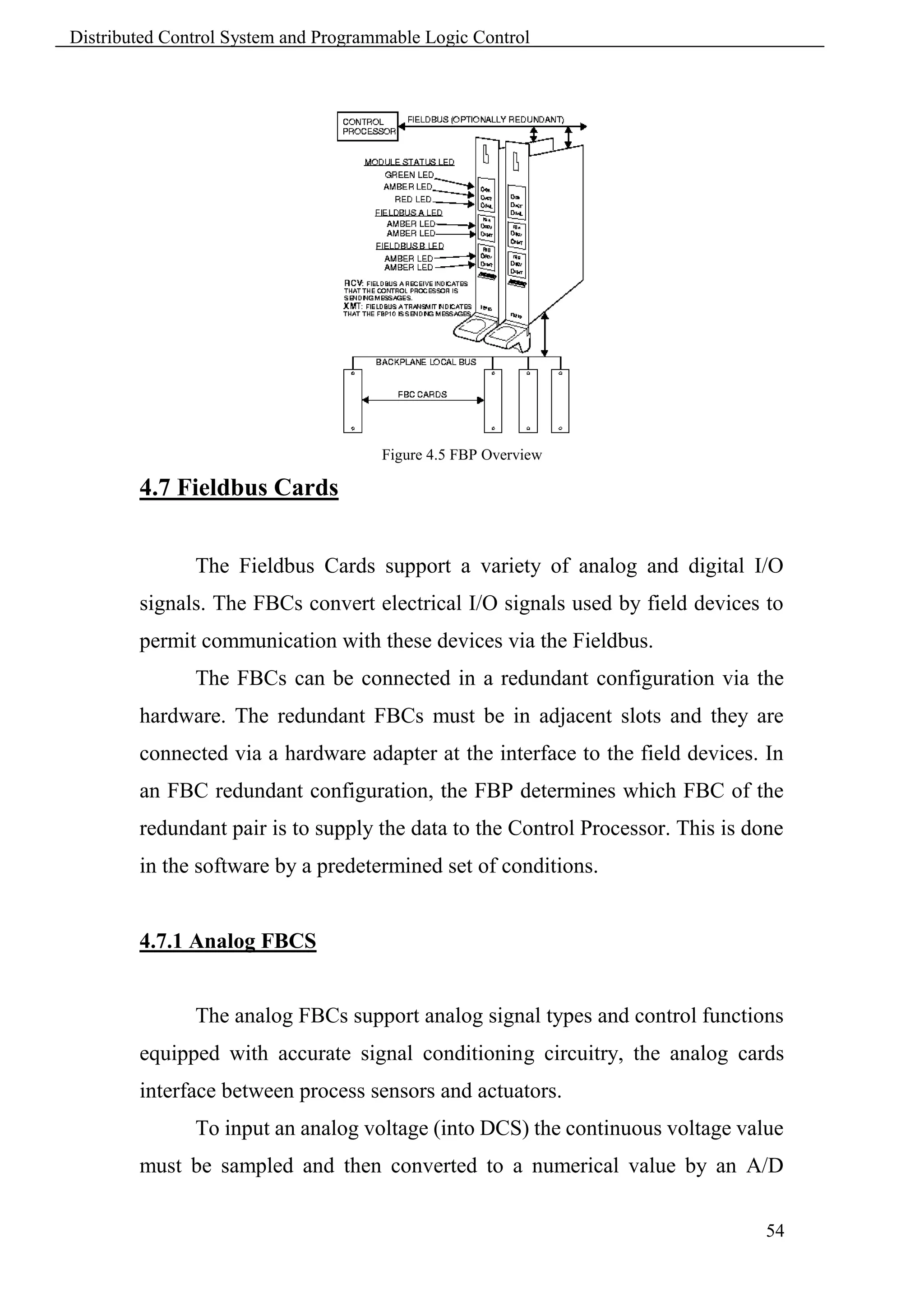
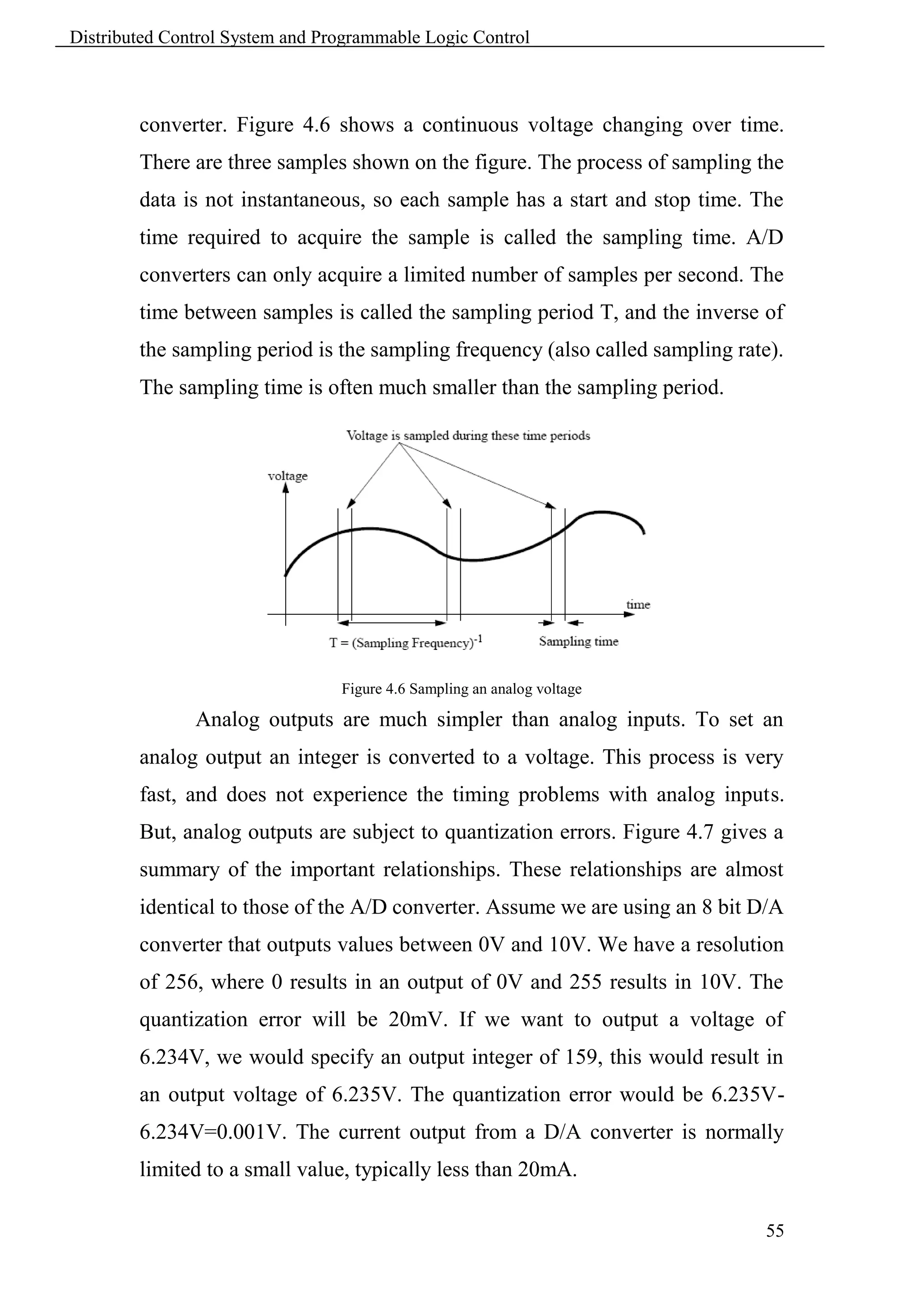
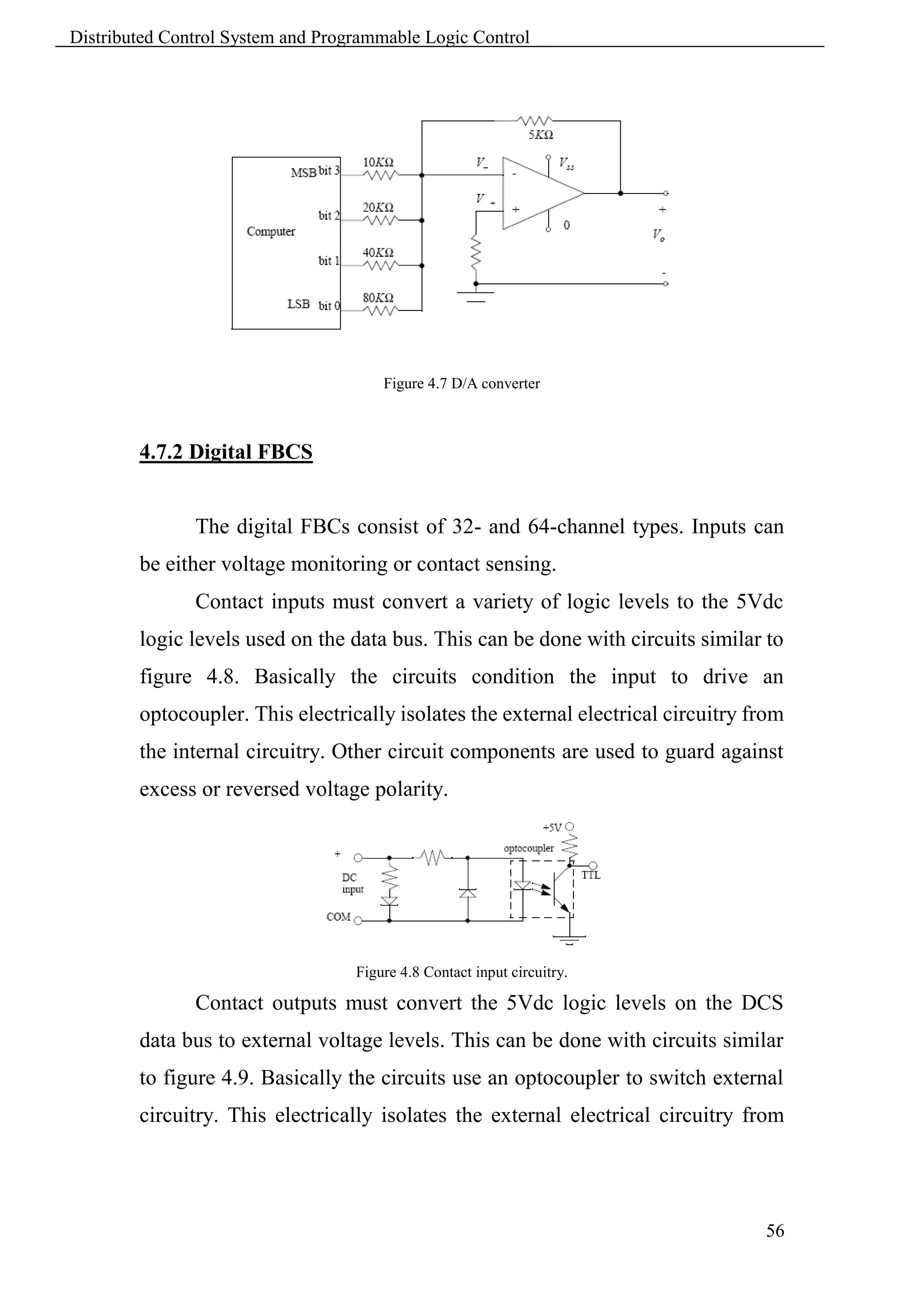
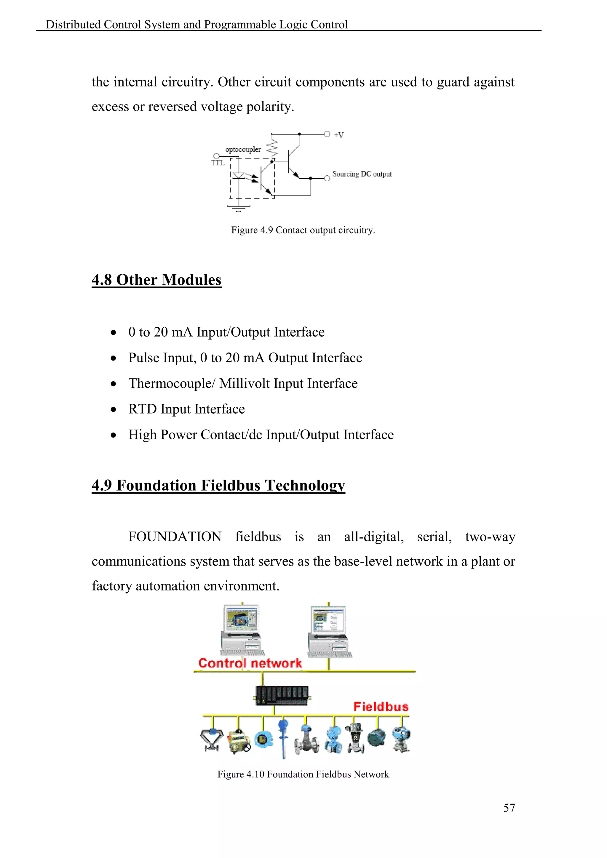
![Distributed Control System and Programmable Logic Control
Knowledge and Elements
Illustrate DCS & PLC Benefits, Usage and History.
Overview of control system history.
Control system benefits and usage.
Types of control
Develop Knowledge of DCS Components (Hardware & Software).
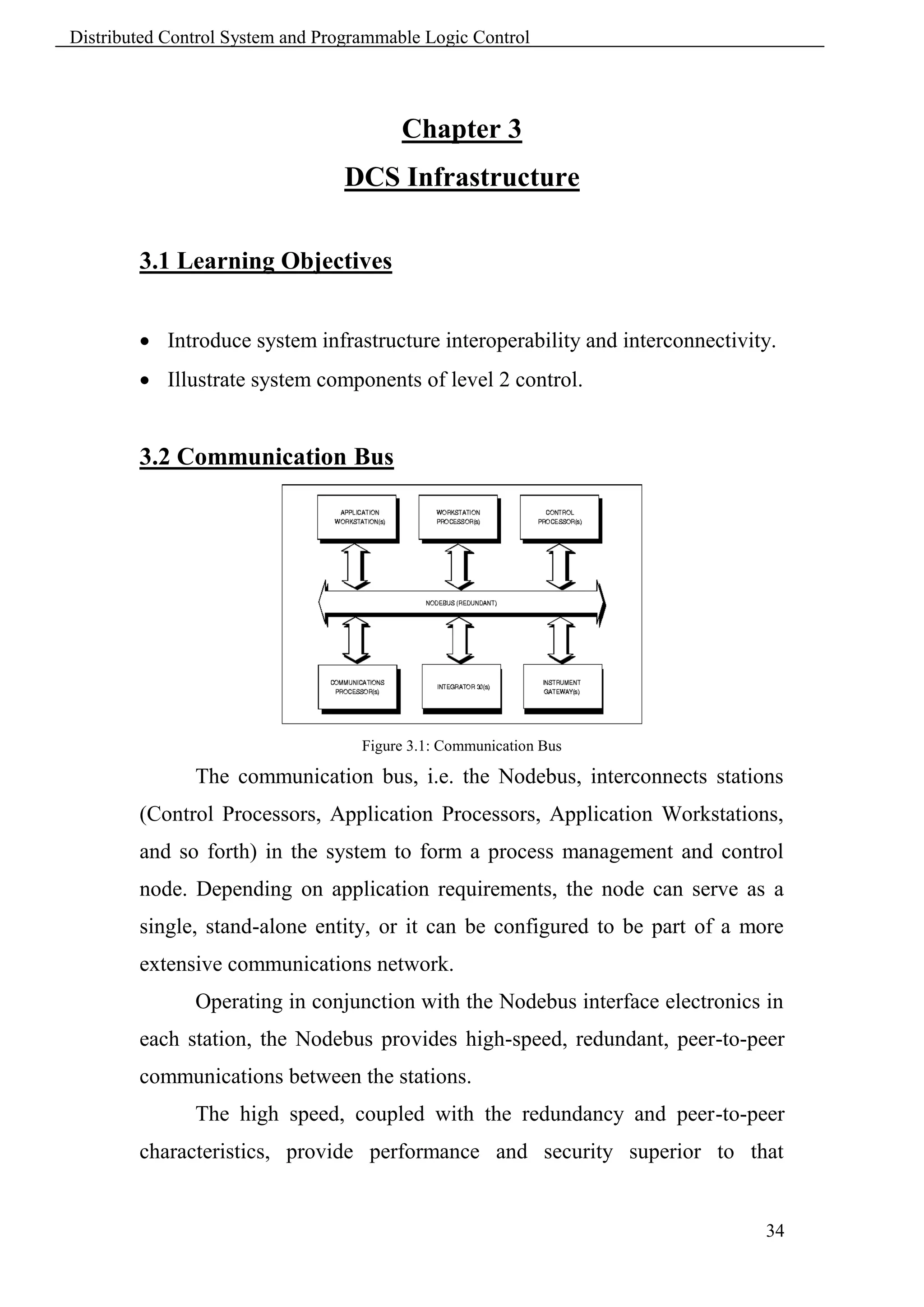
Infrastructure [Communication Bus, Interfaces, Controllers,
Gateways, RTU, Others].
Hardware and technologies.
Software [Configuration, Graphics, Alarming, Trending, System
Management, Others].
Extend Knowledge of DCS installation and Maintenance.
Site Installation, Commissioning and Startup.
Diagnostics, Spares, Tools and Power Distribution.
Maintenance [Backup, Replacements and System Installation].
Develop Knowledge of PLC Components.
PLC fundamentals.
PLC Logic.
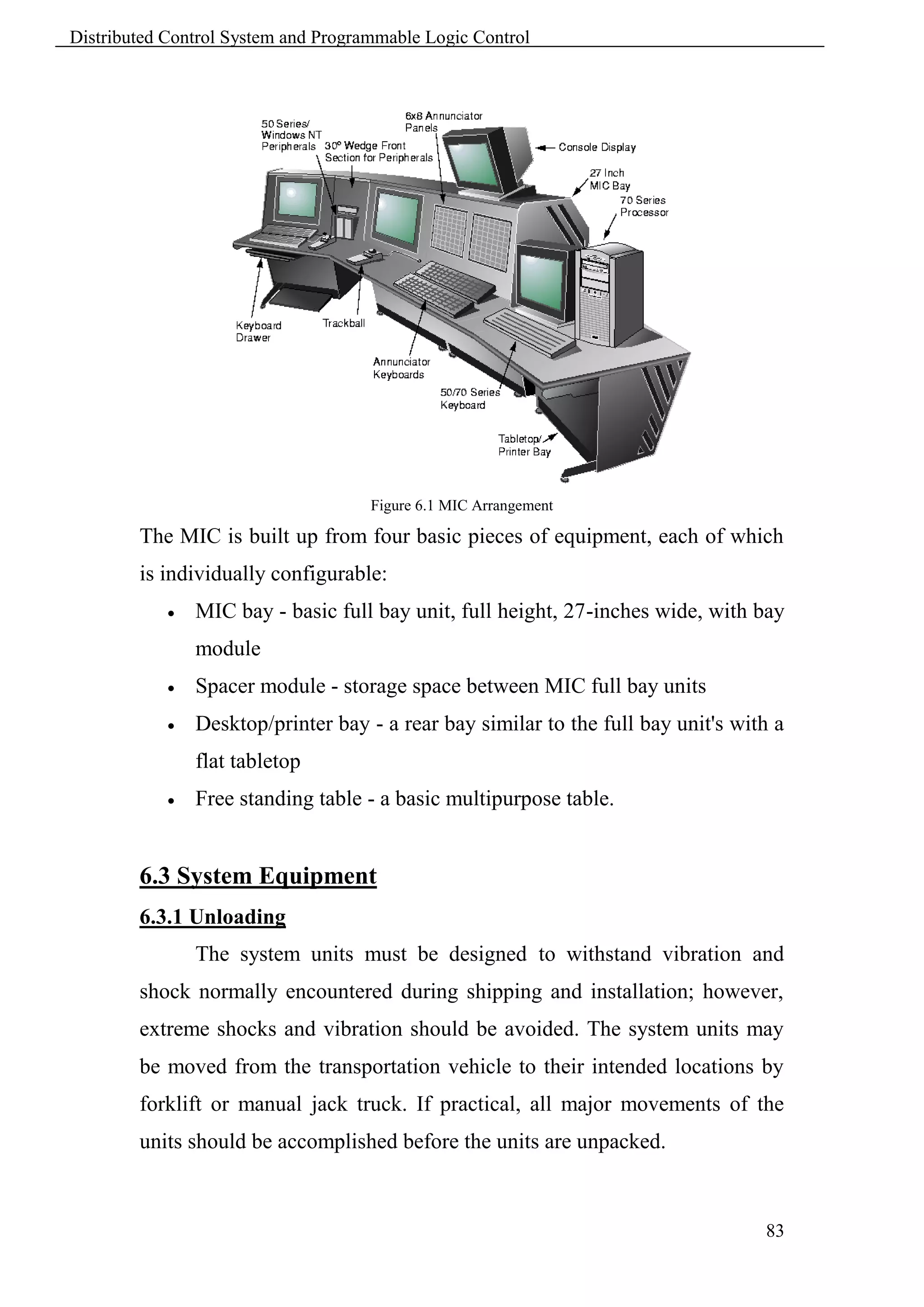
2](https://image.slidesharecdn.com/dcscourse-120105225019-phpapp02/75/Dcs-course-3-2048.jpg)
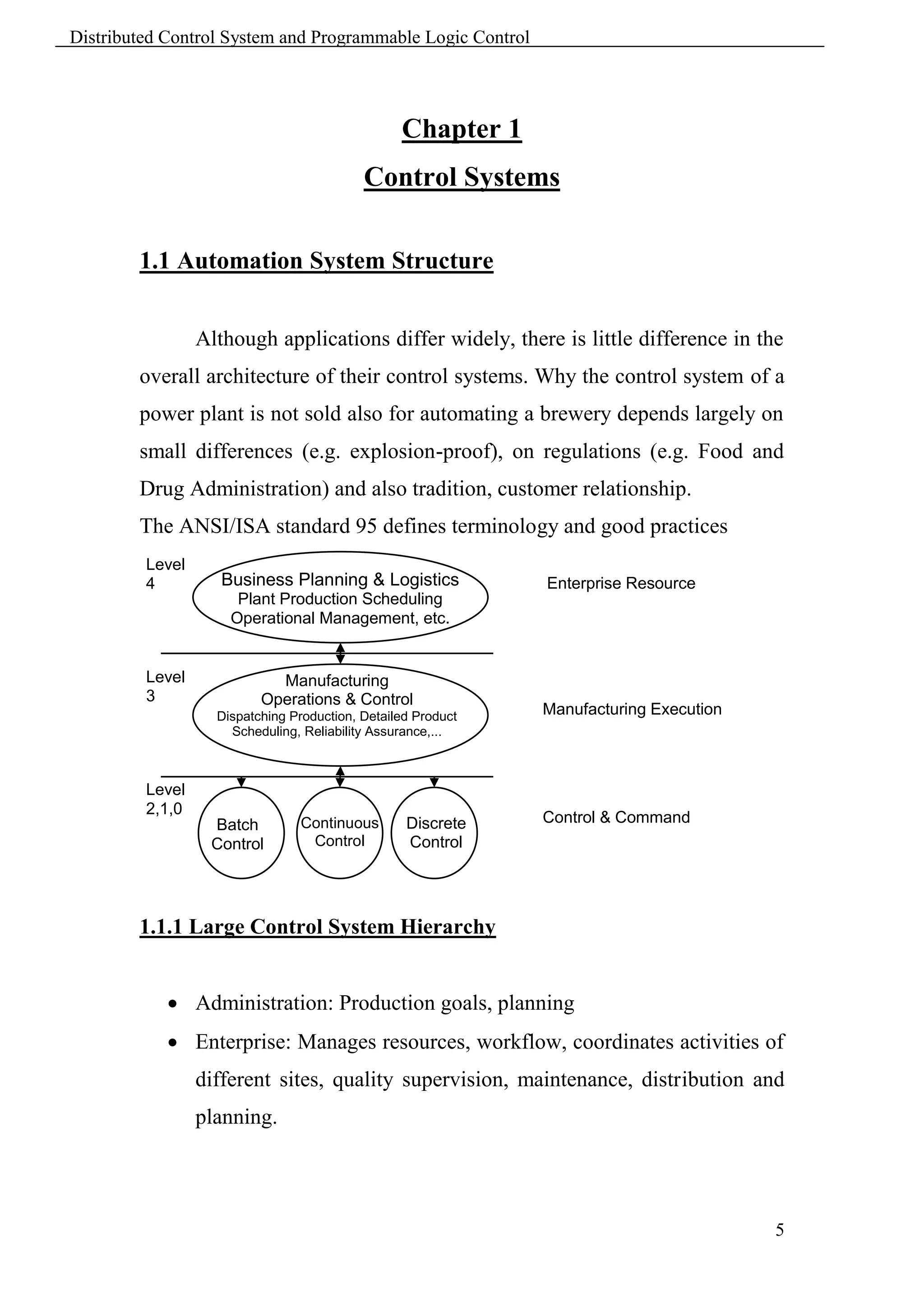
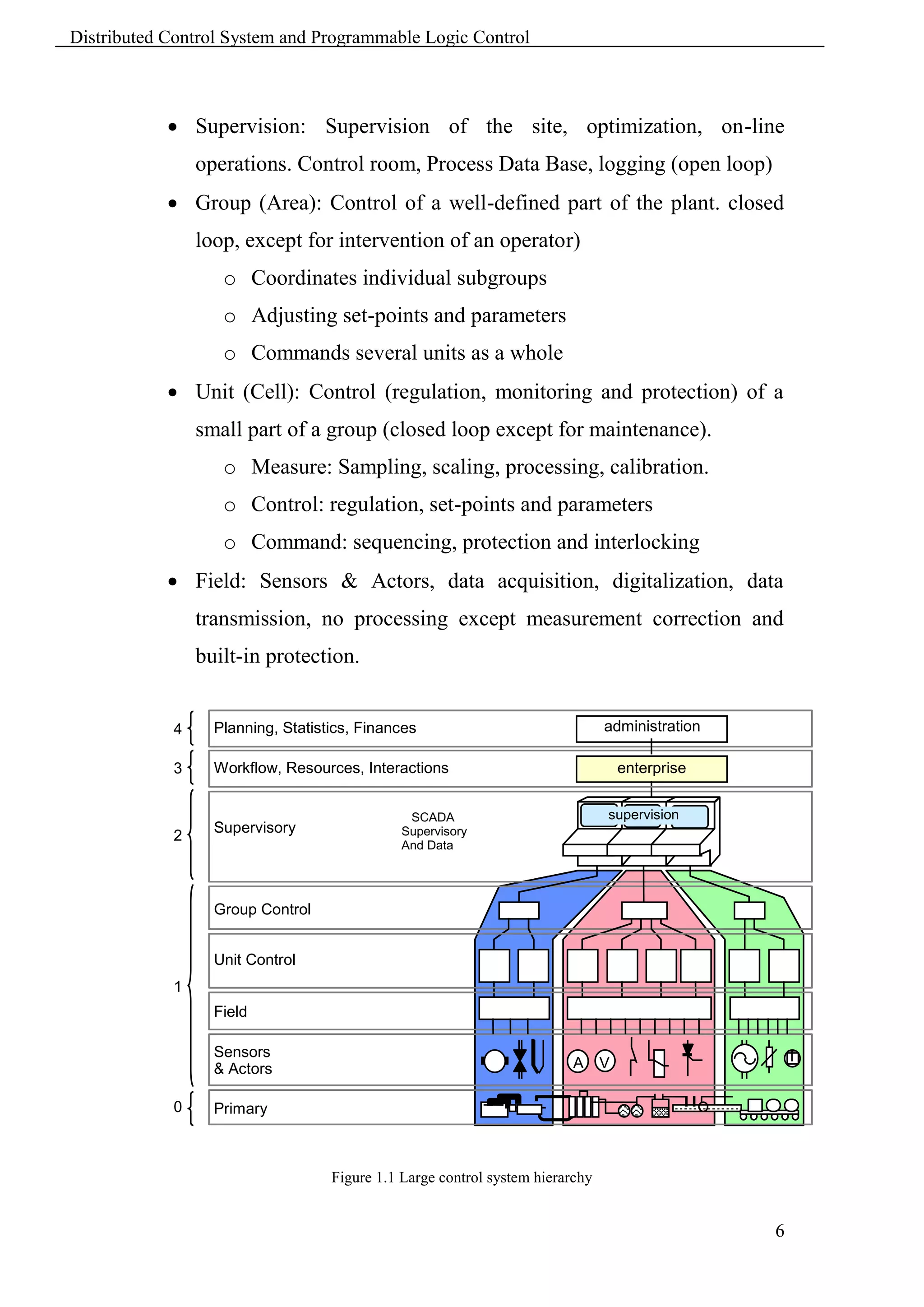
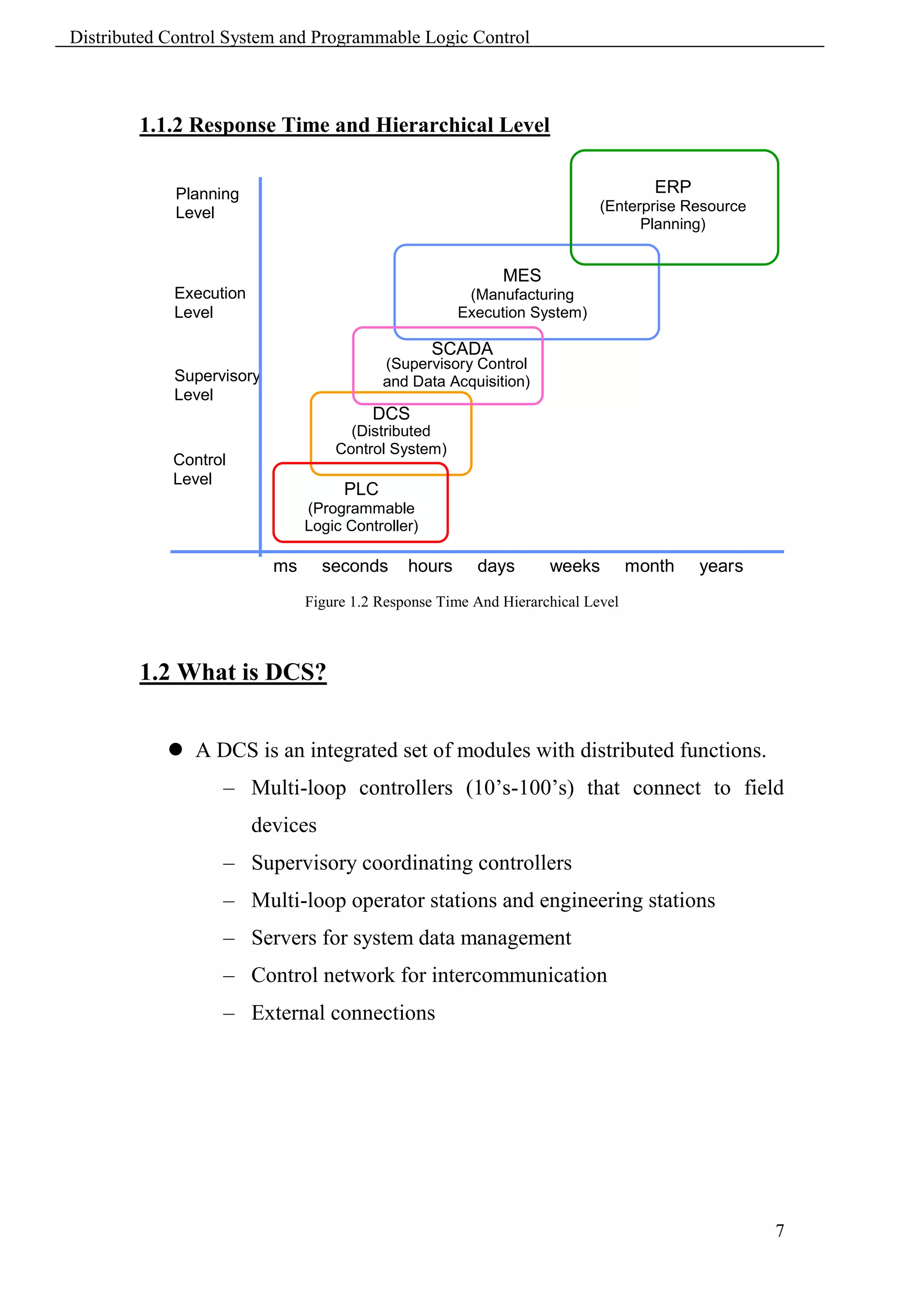
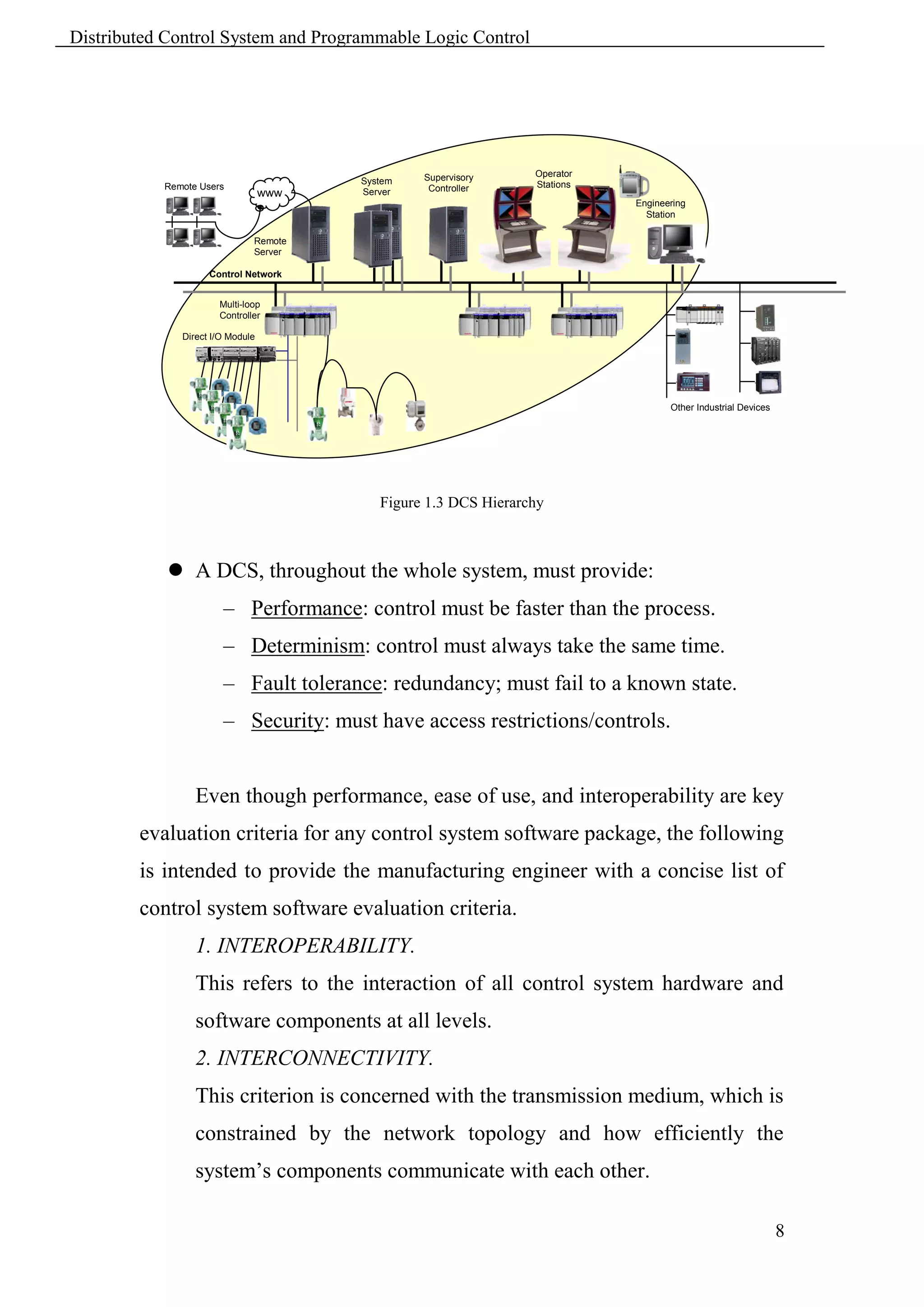

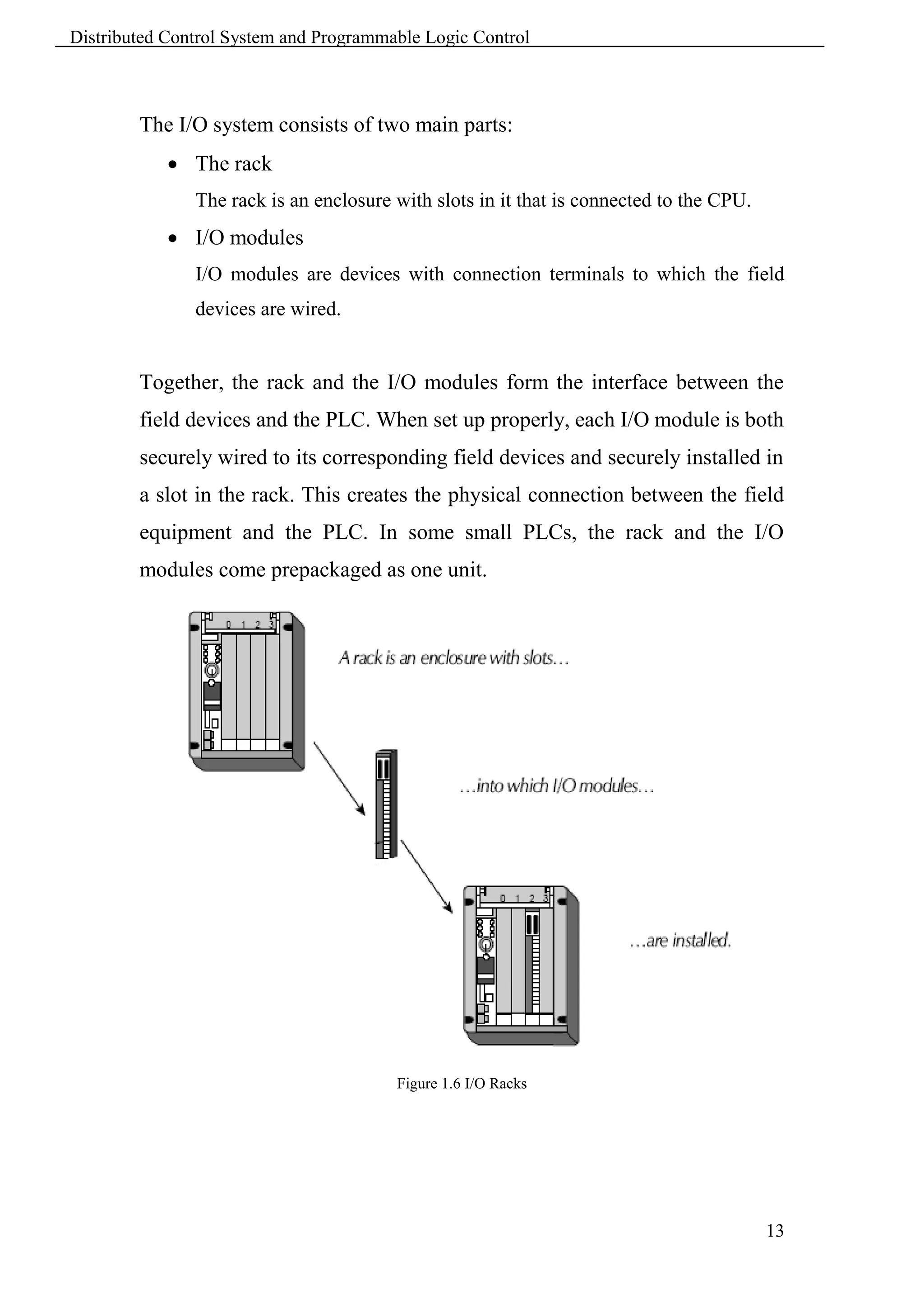
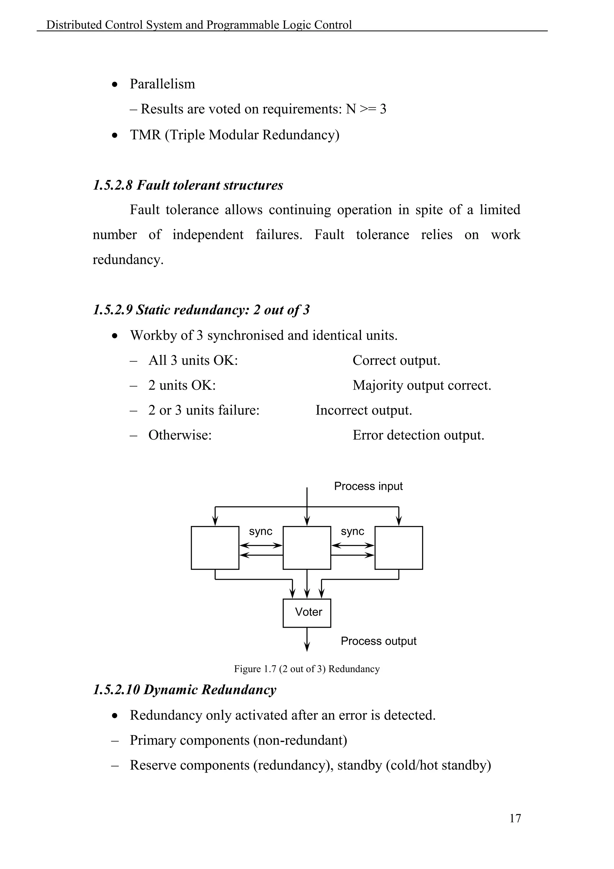
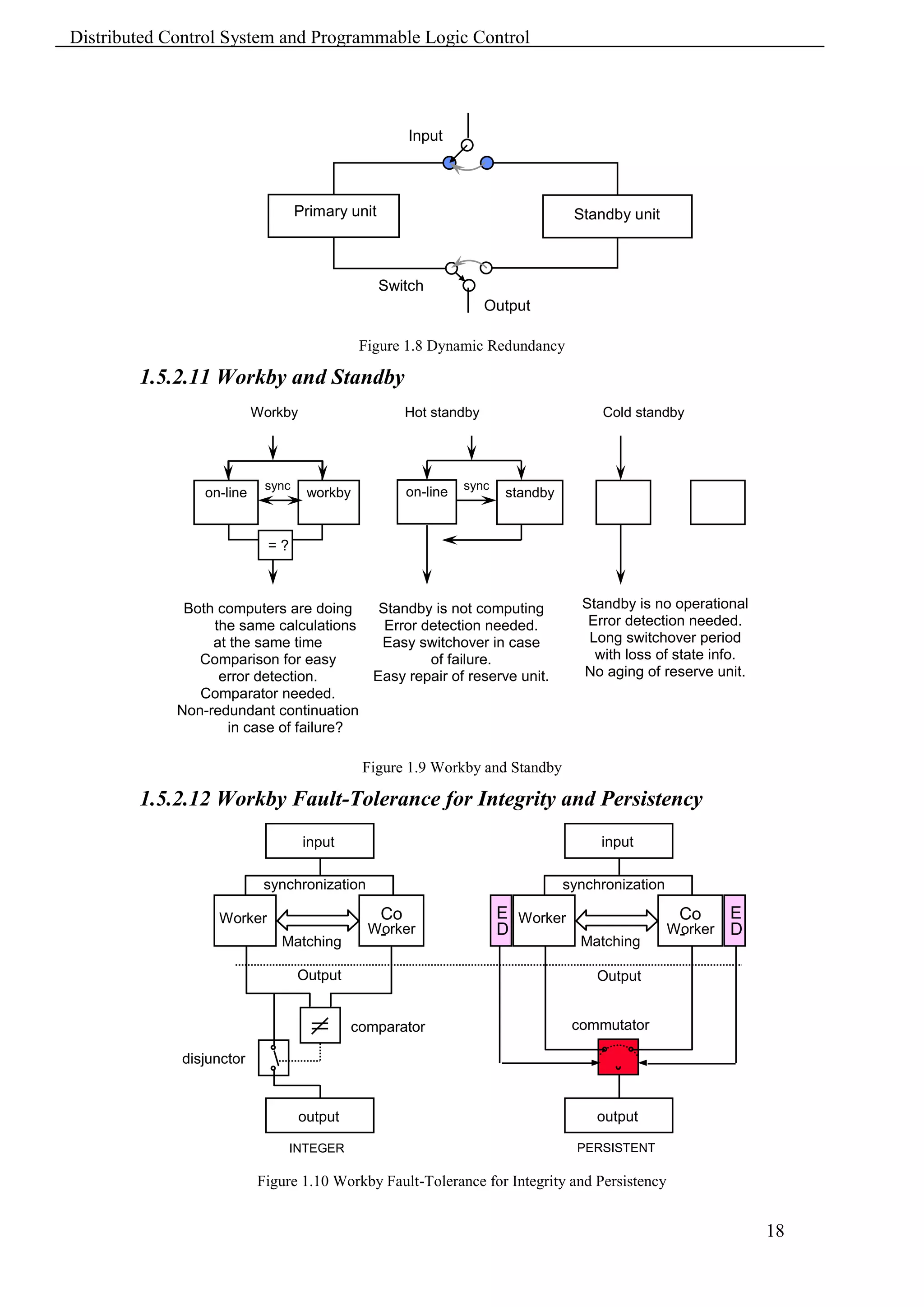
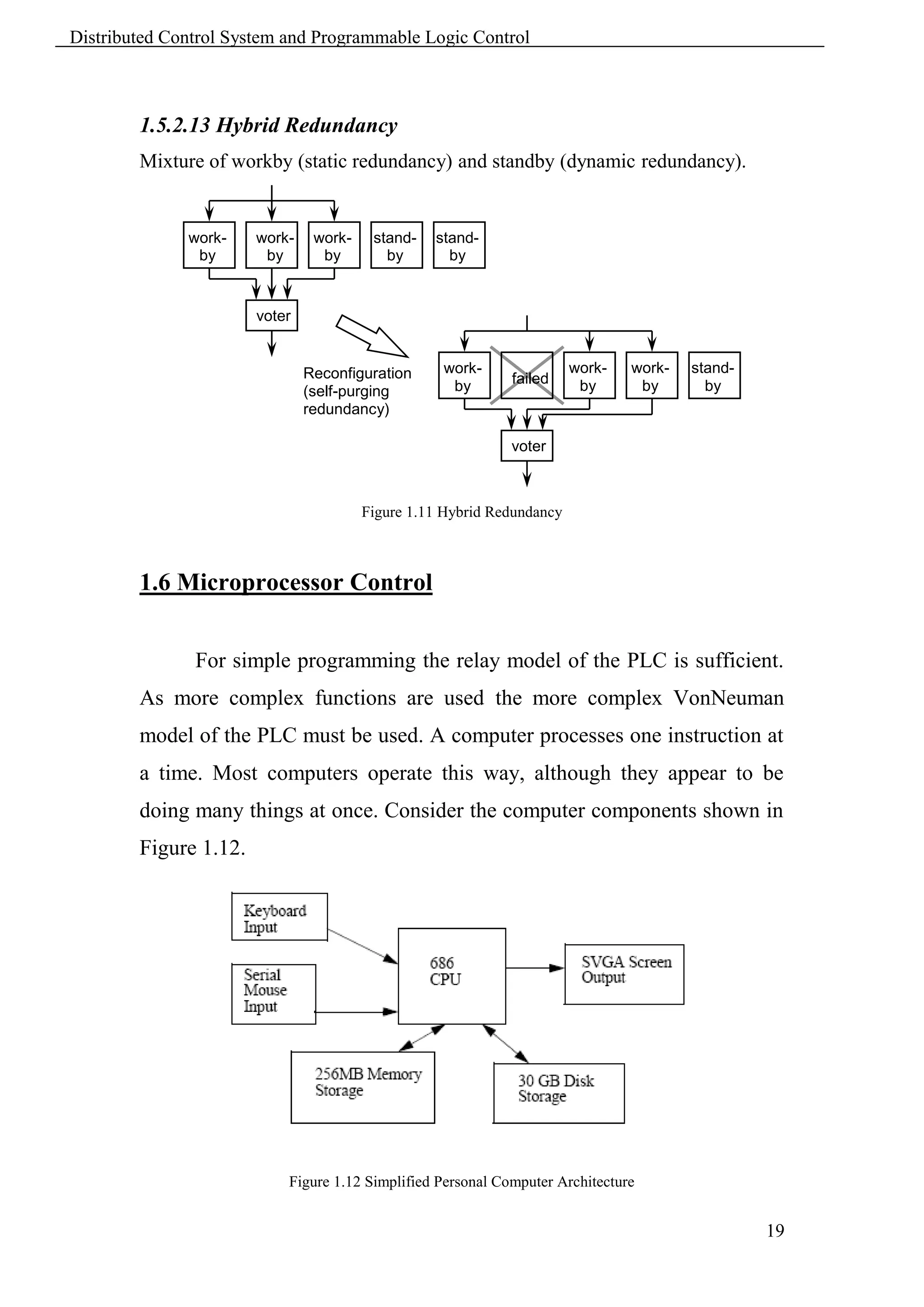
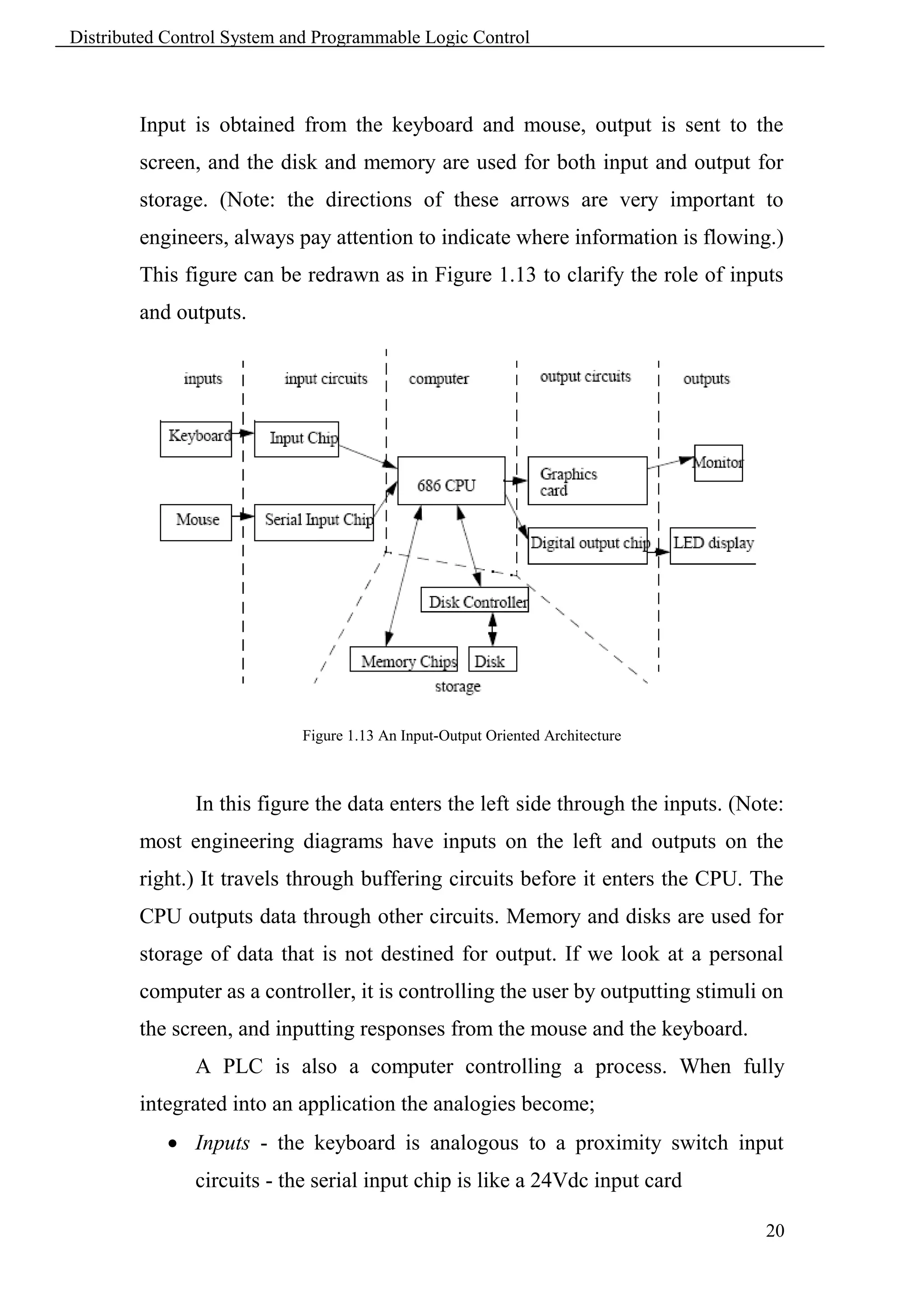
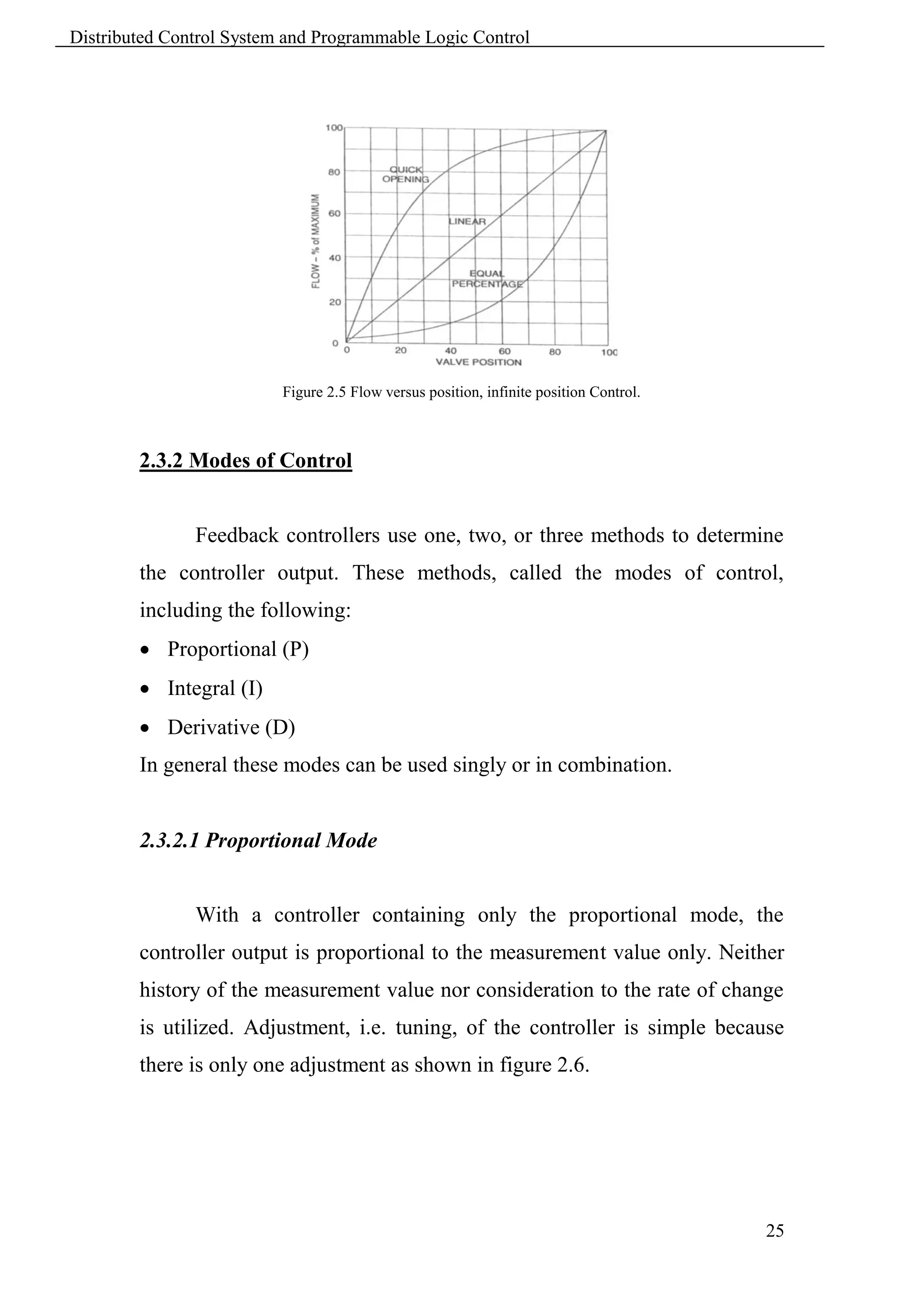
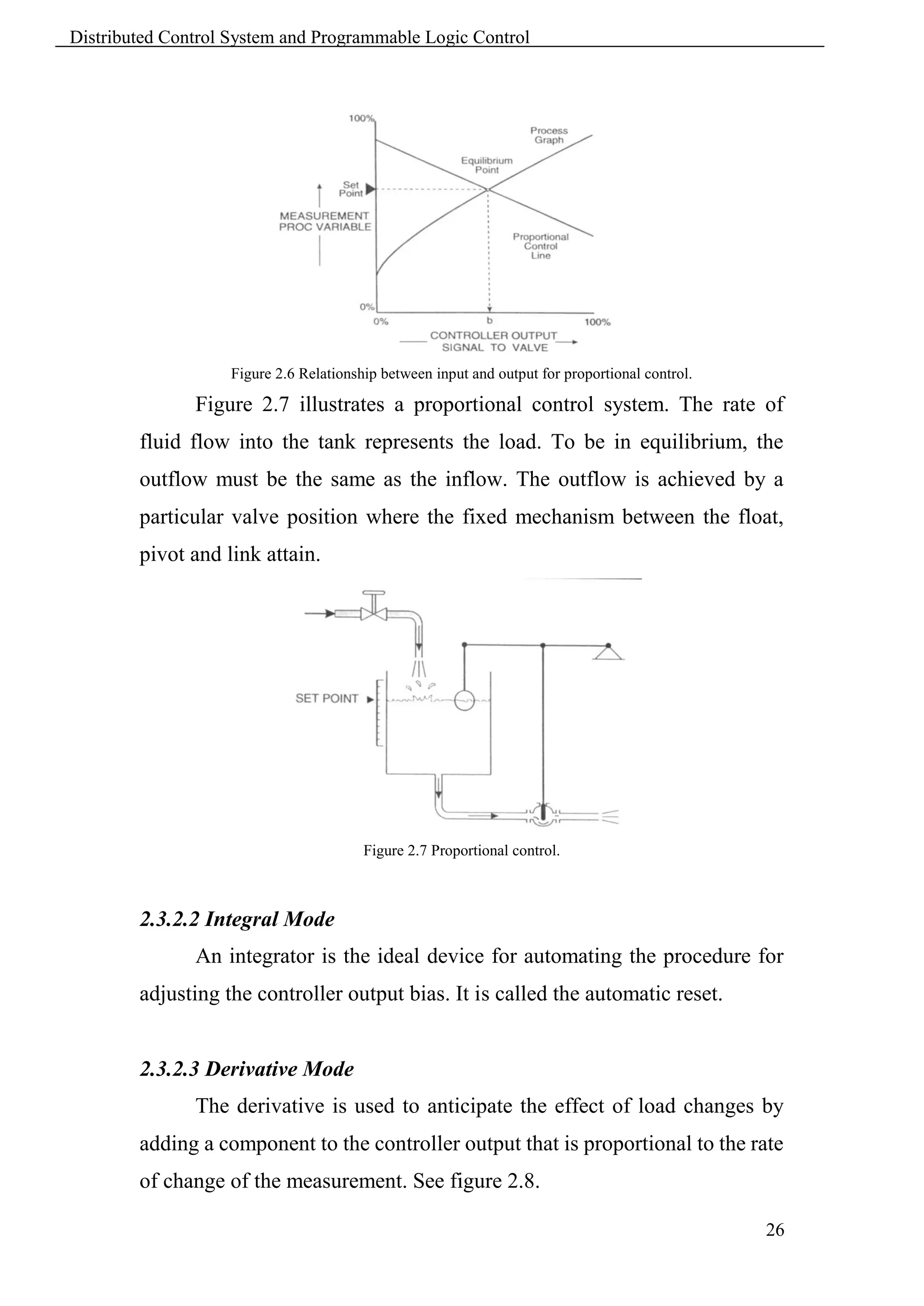
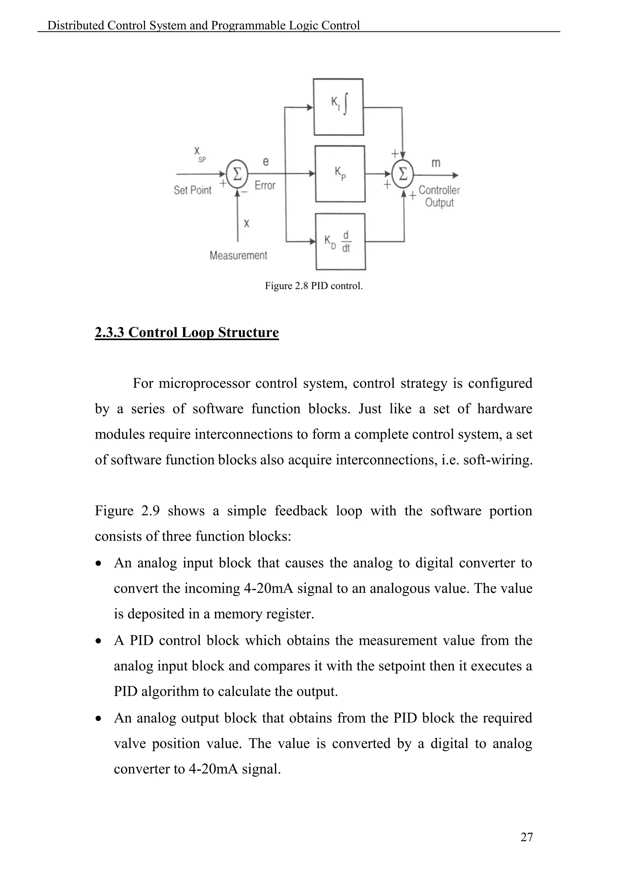
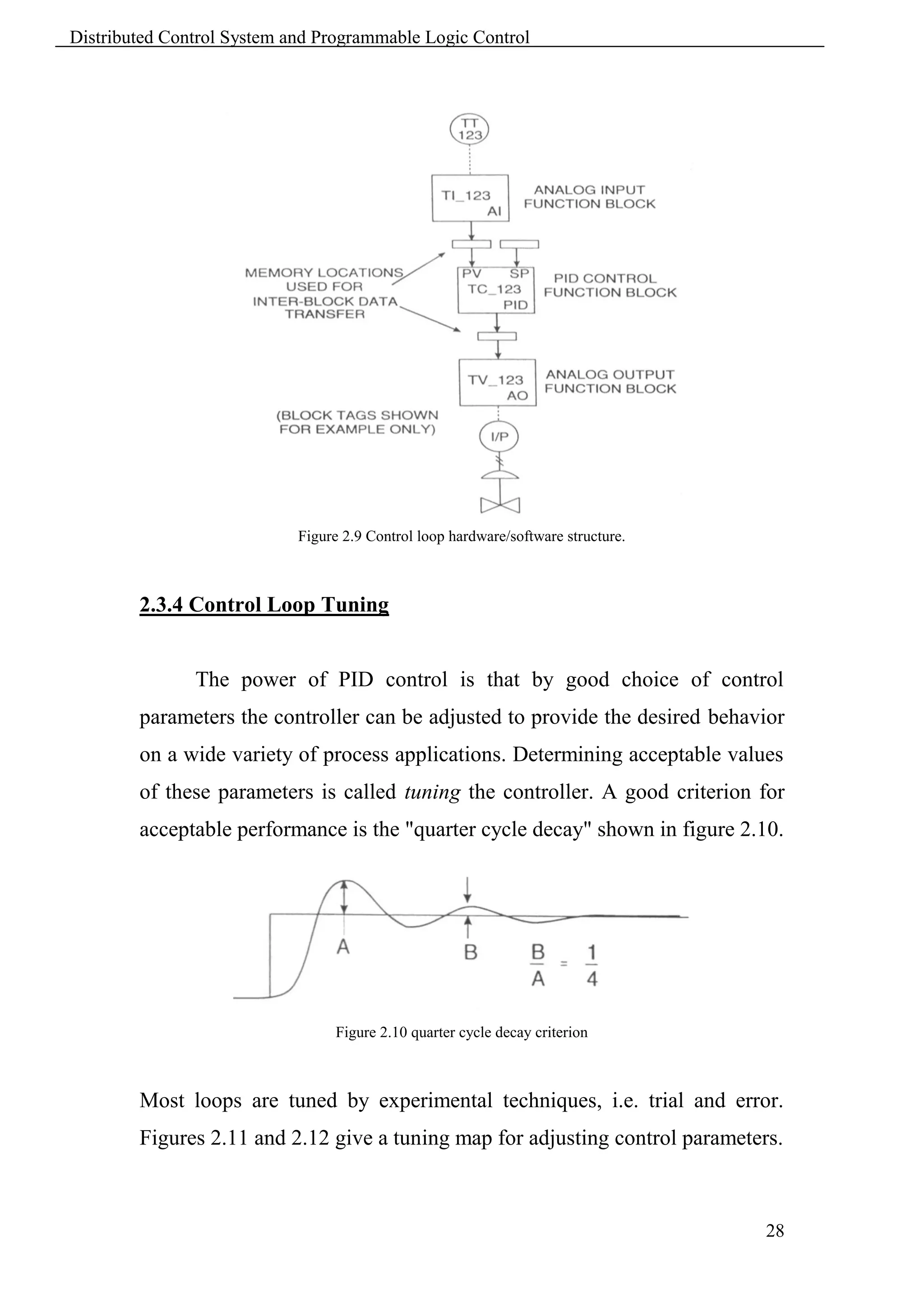
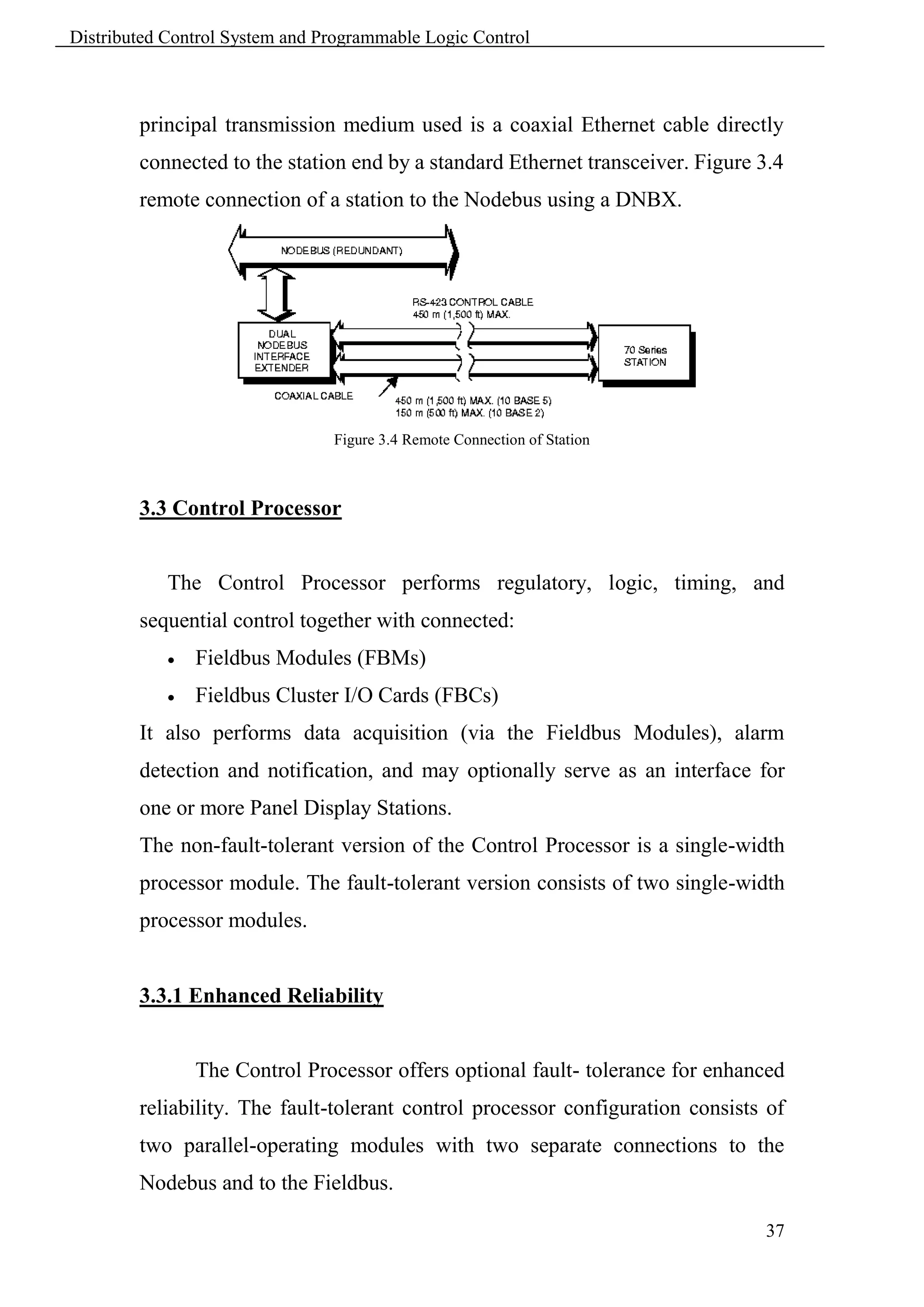

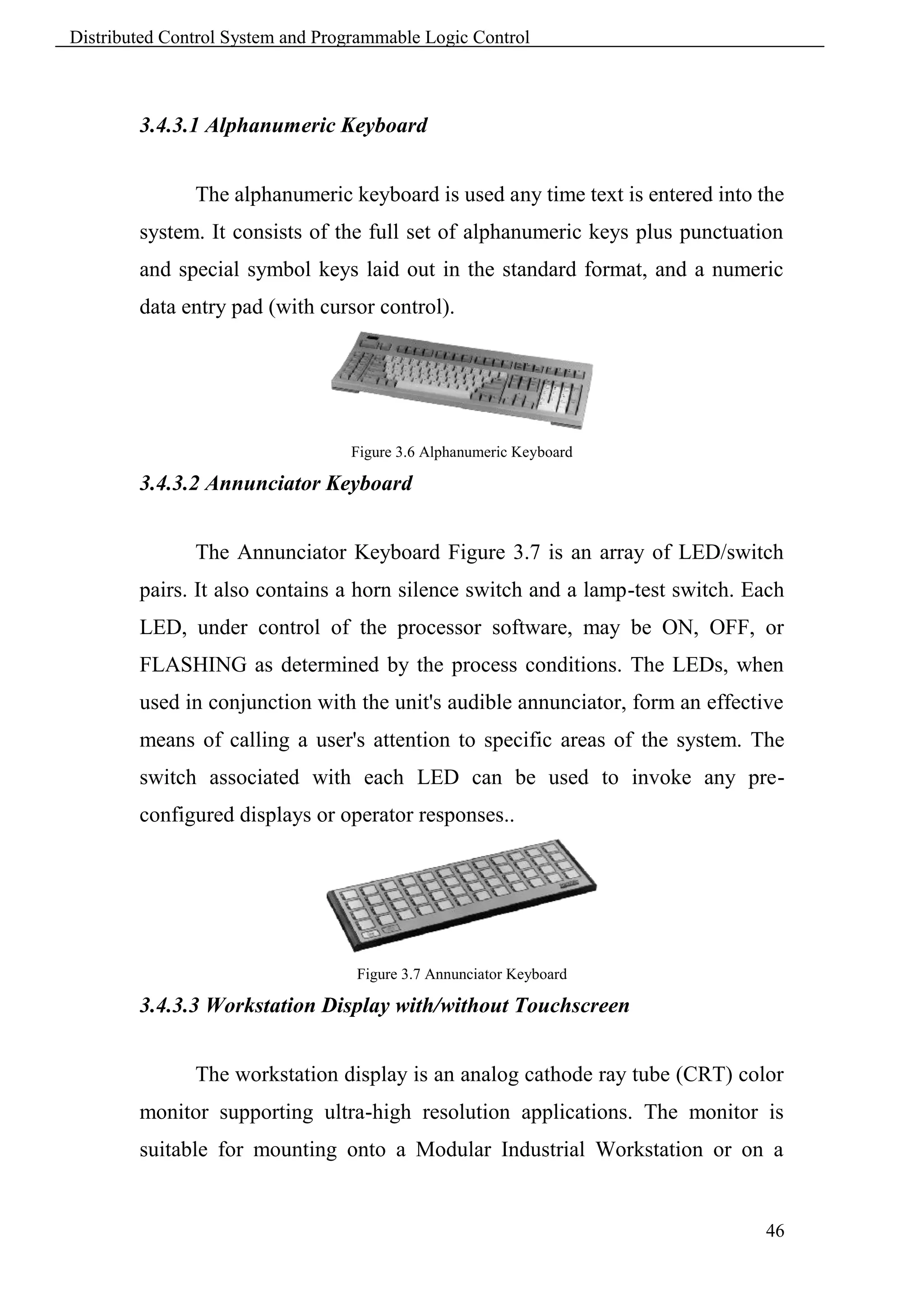
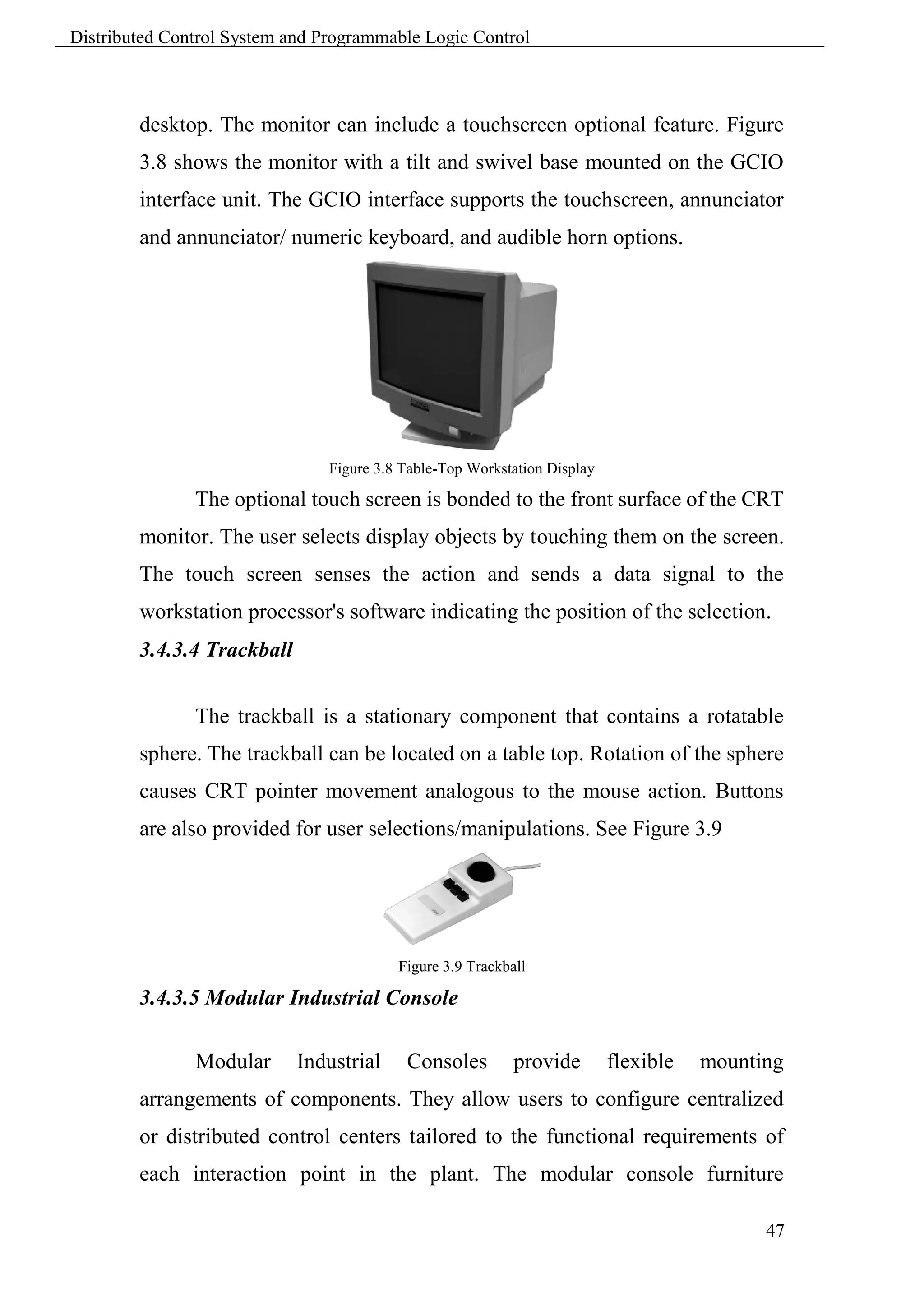
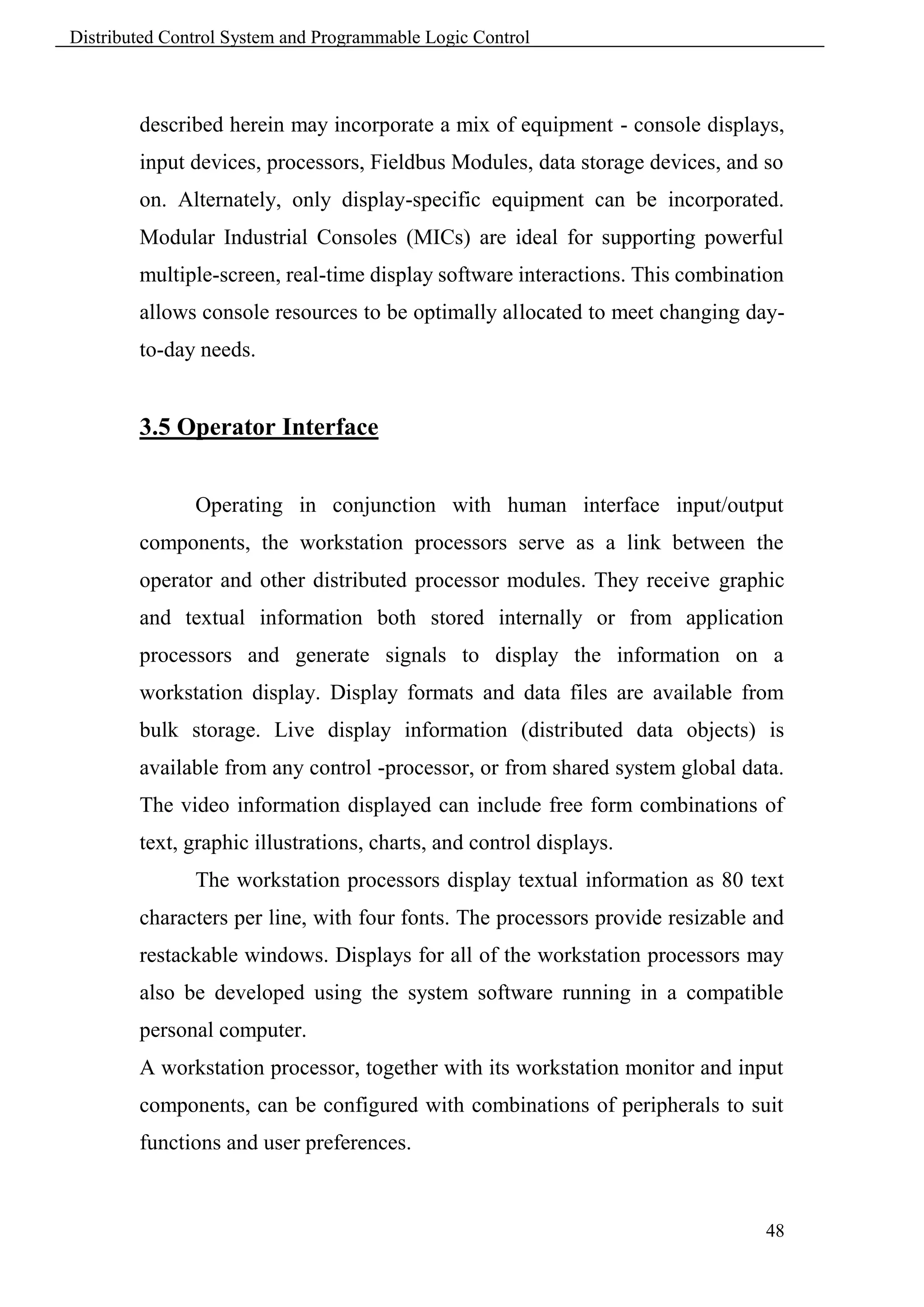
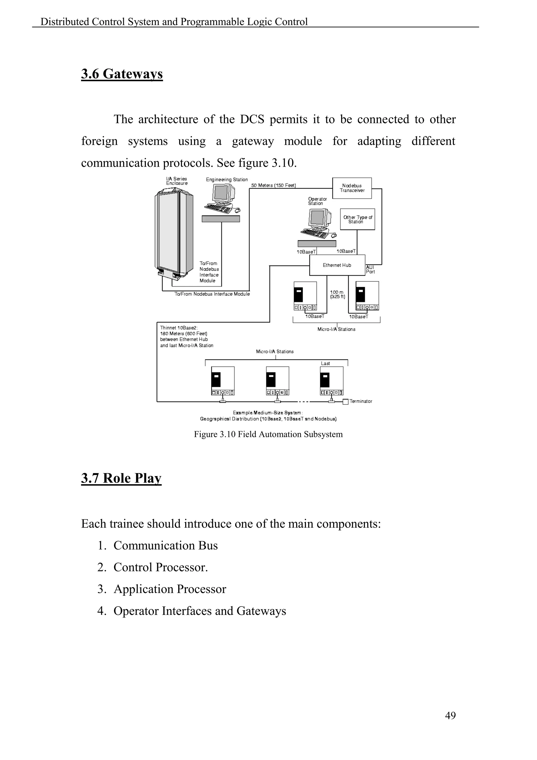
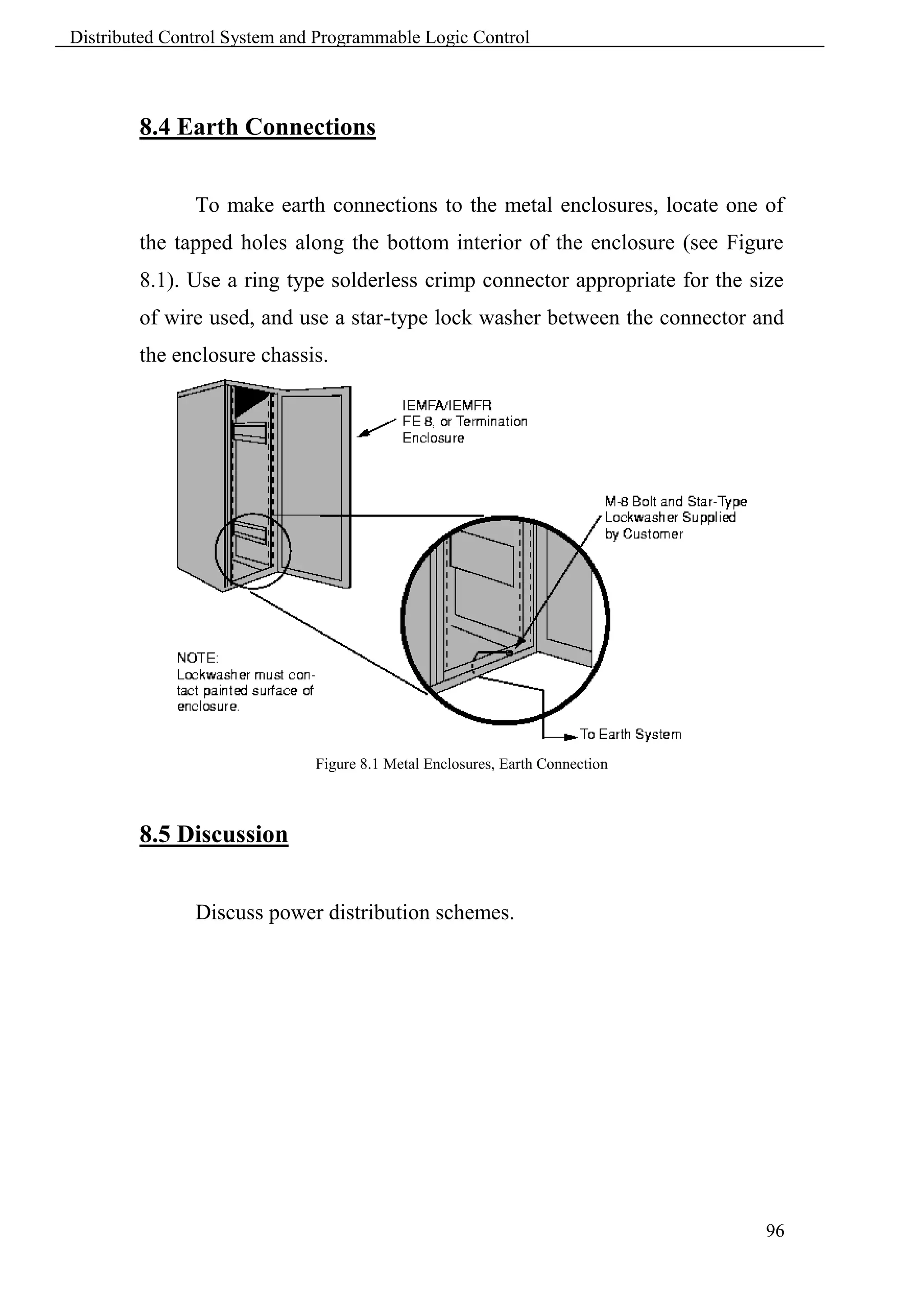
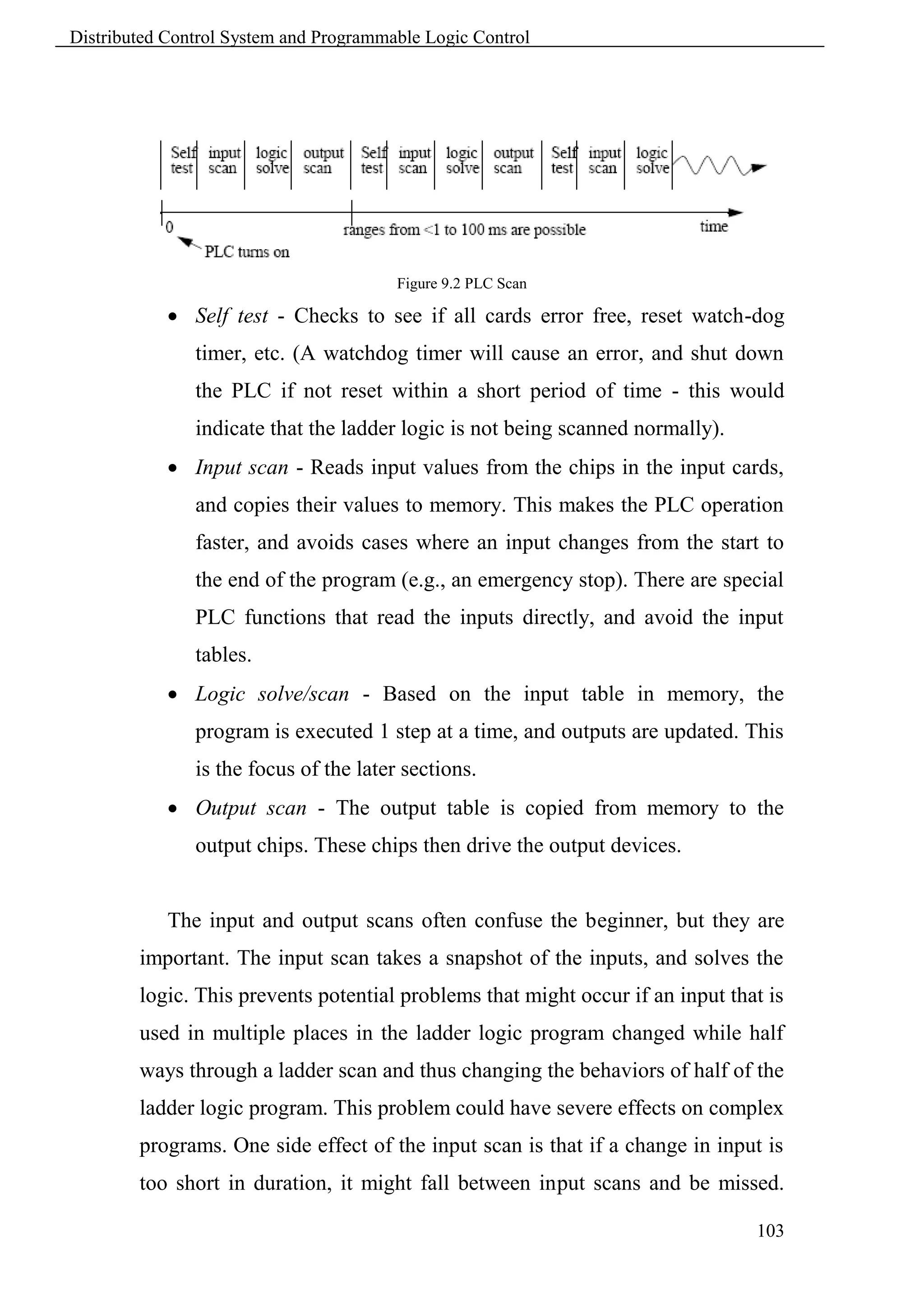
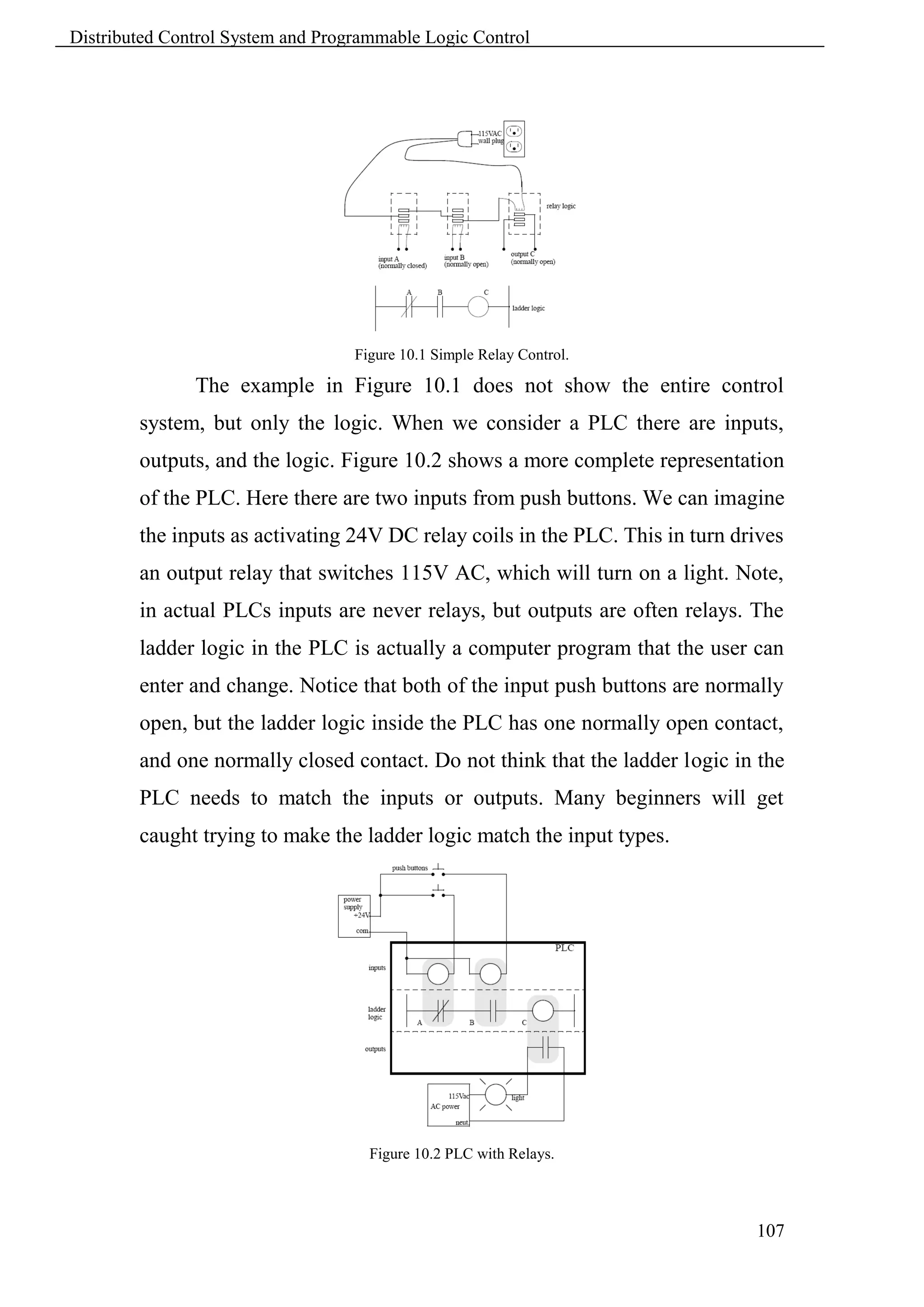
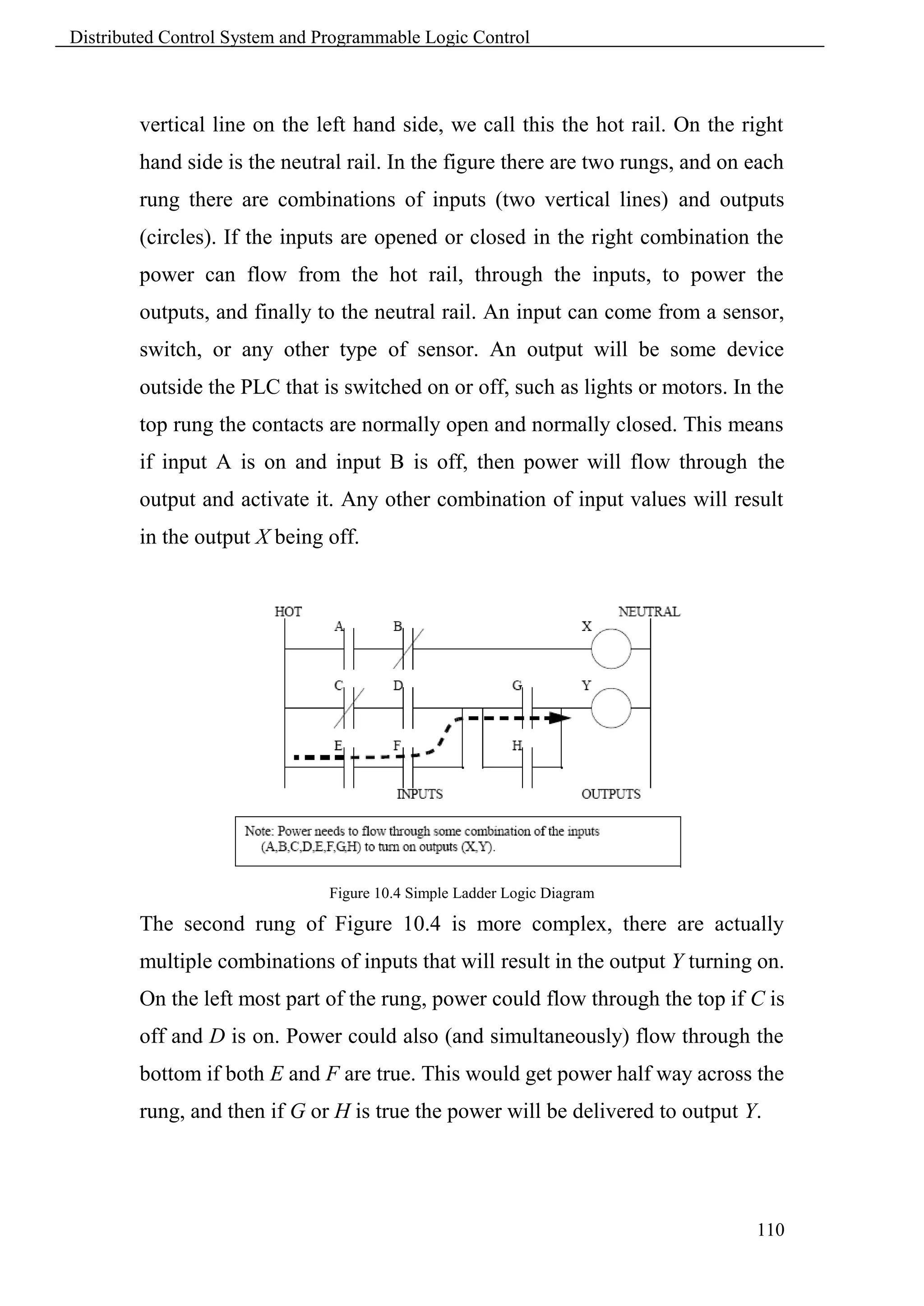
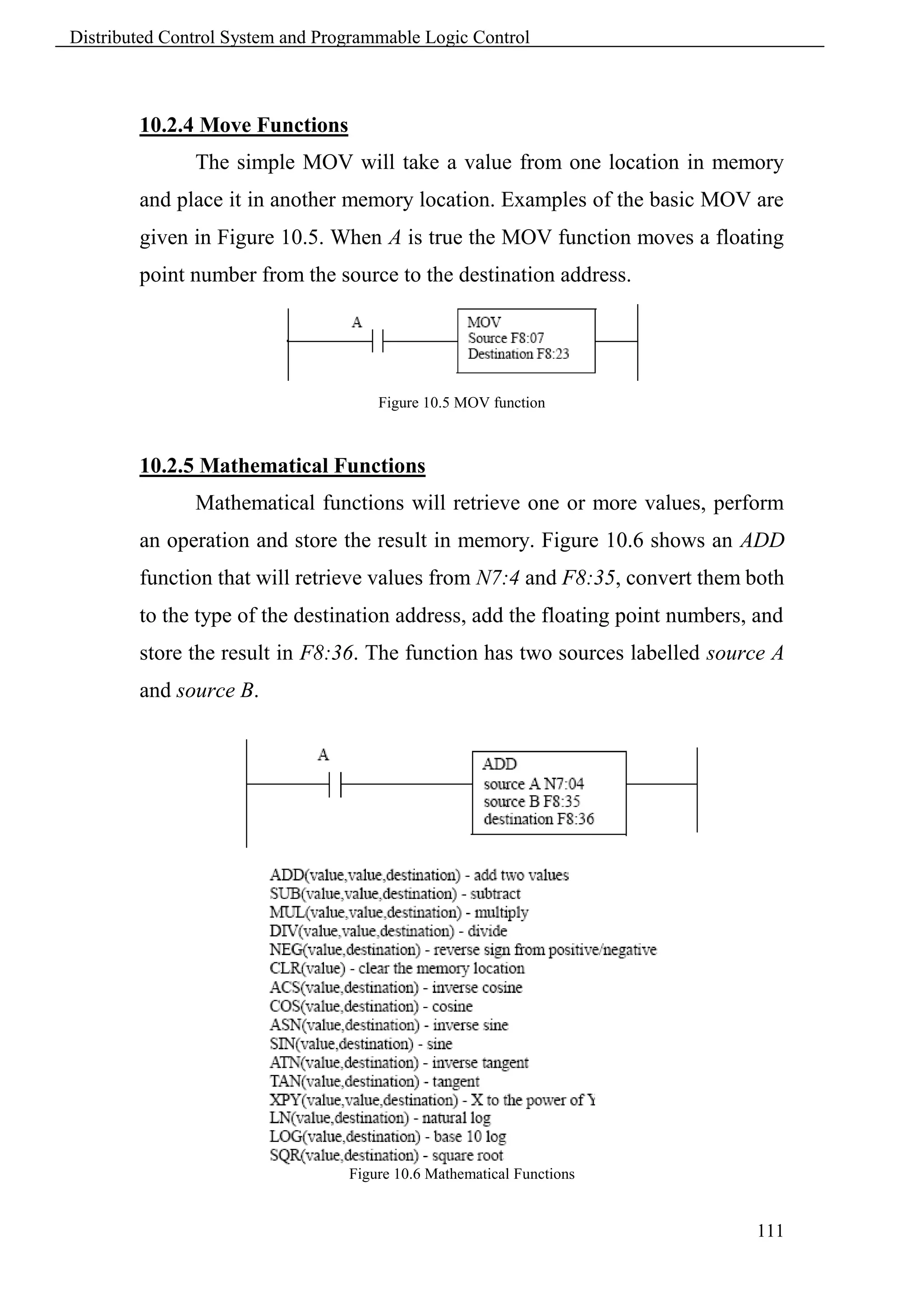
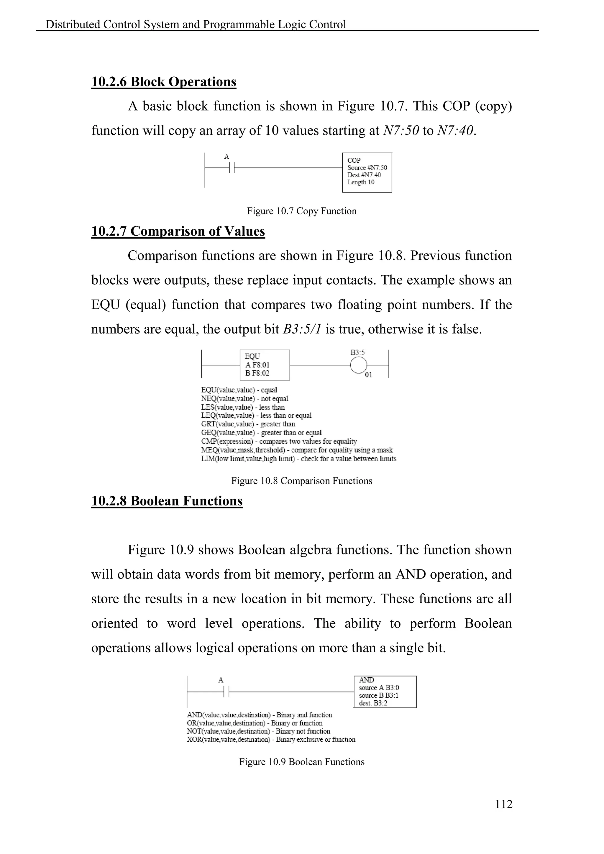
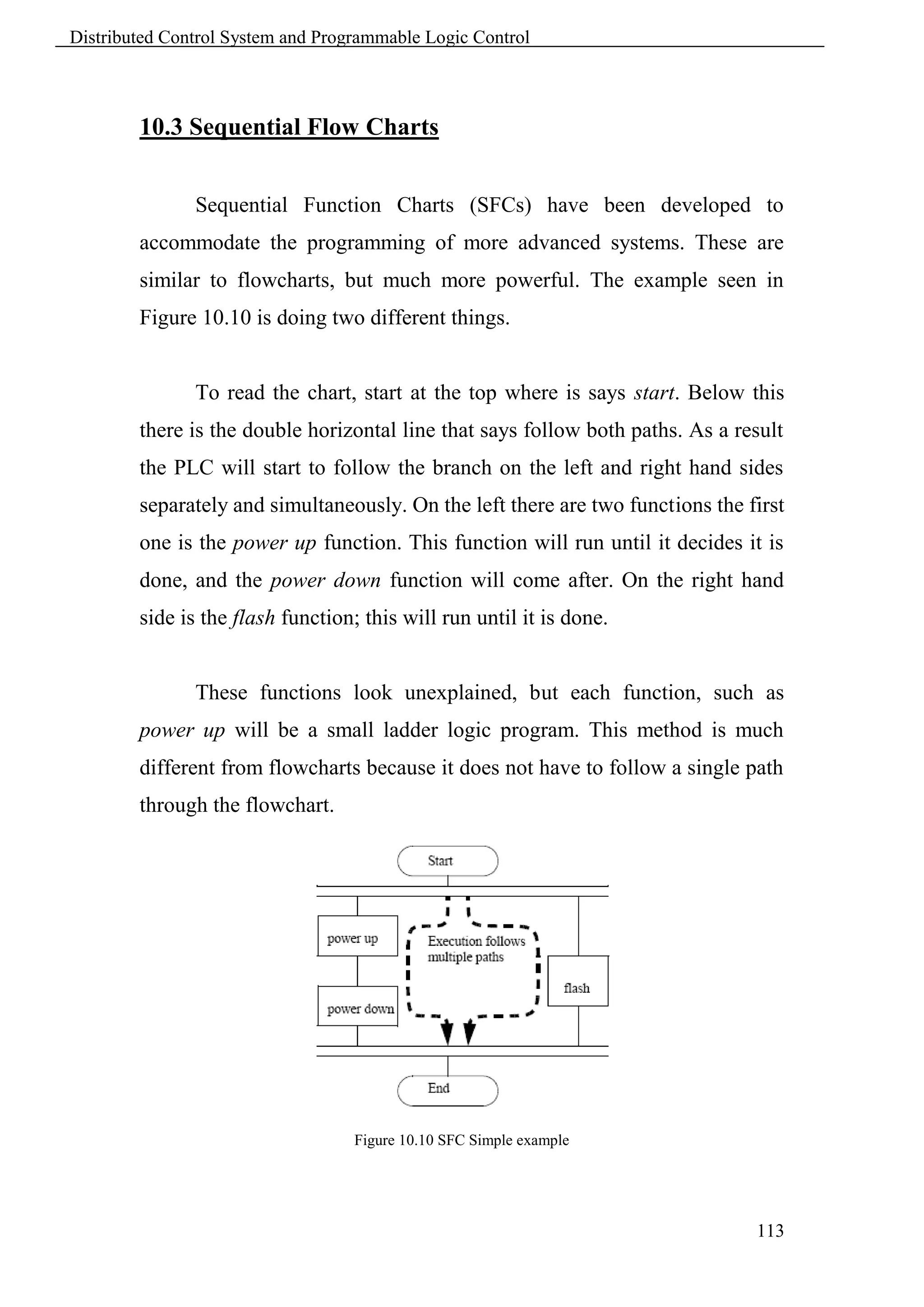
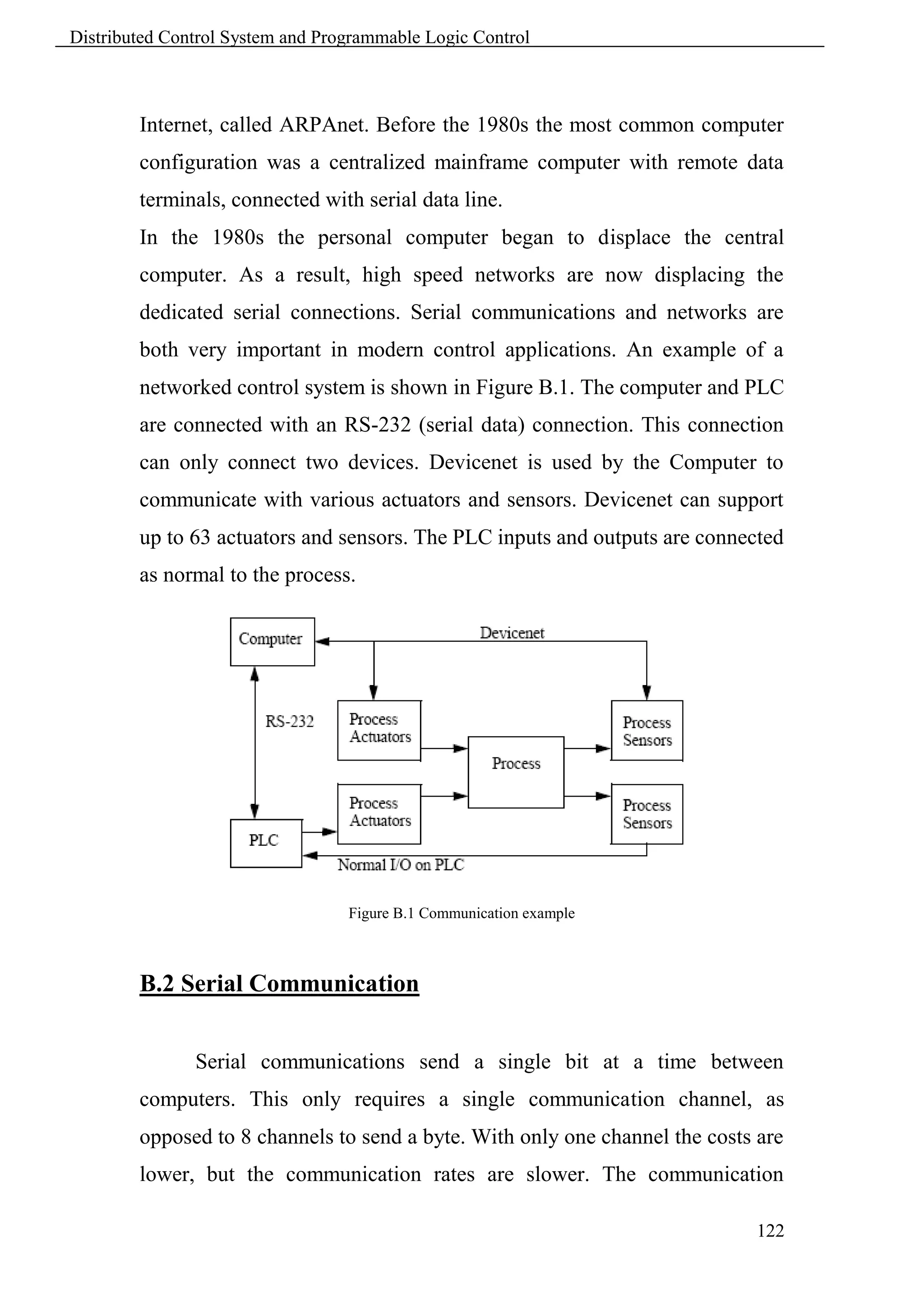
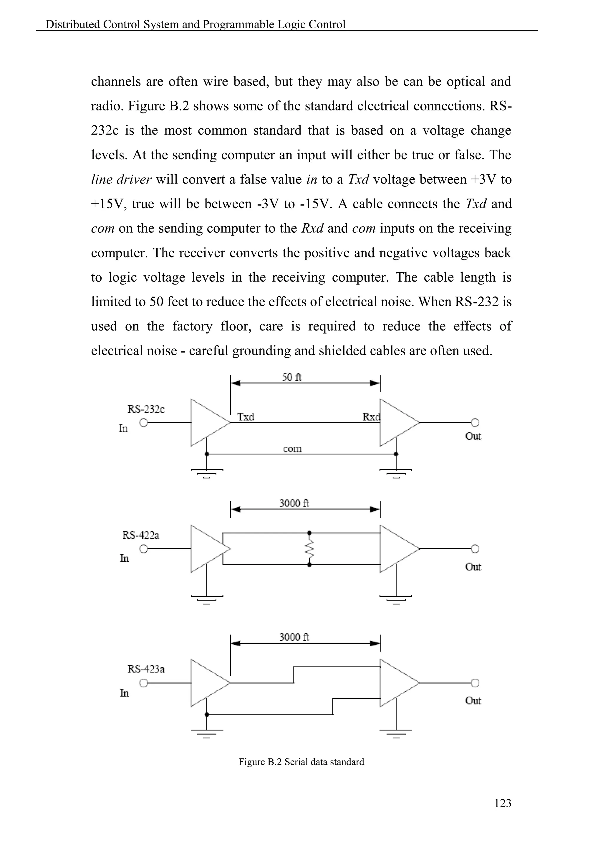
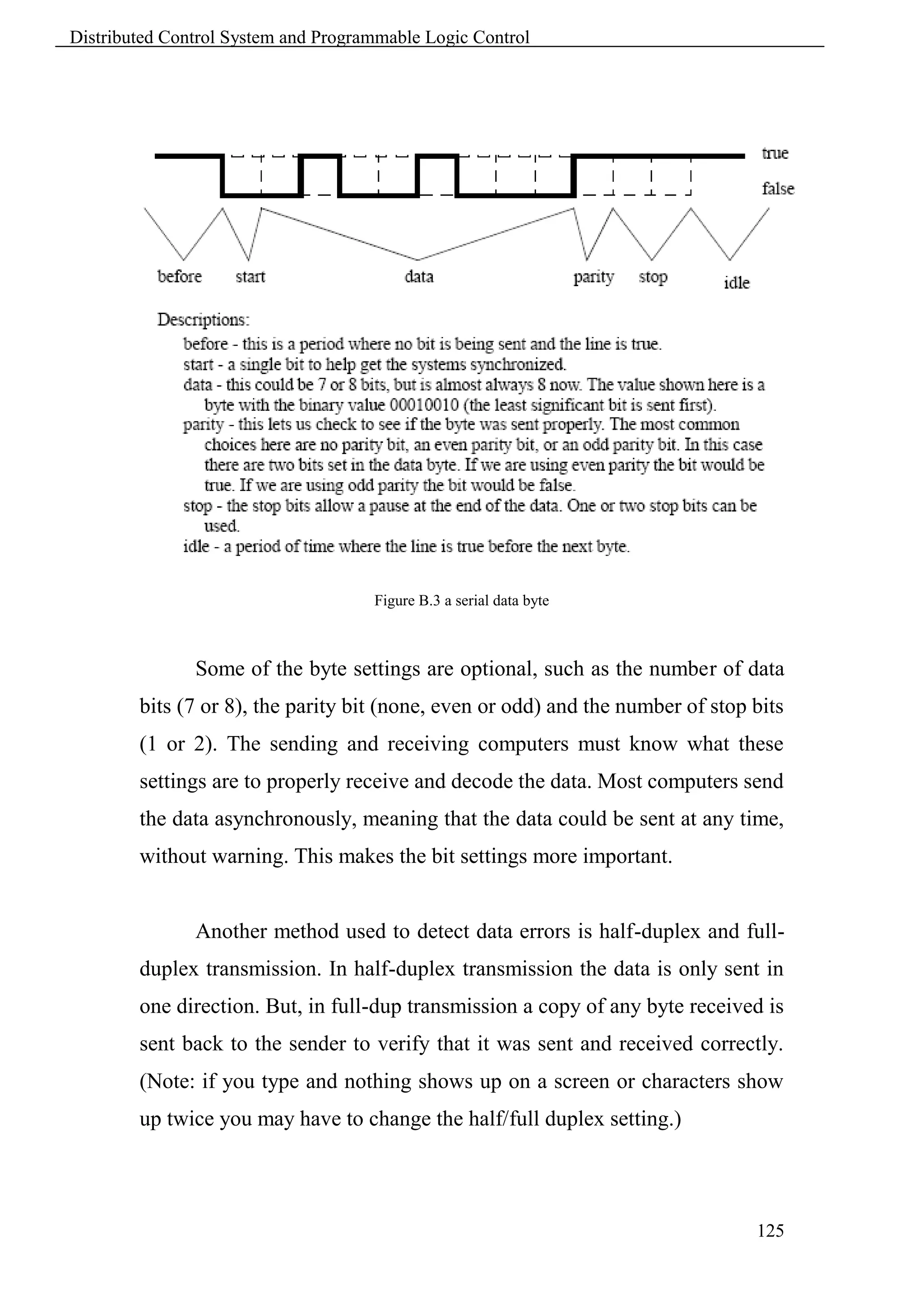
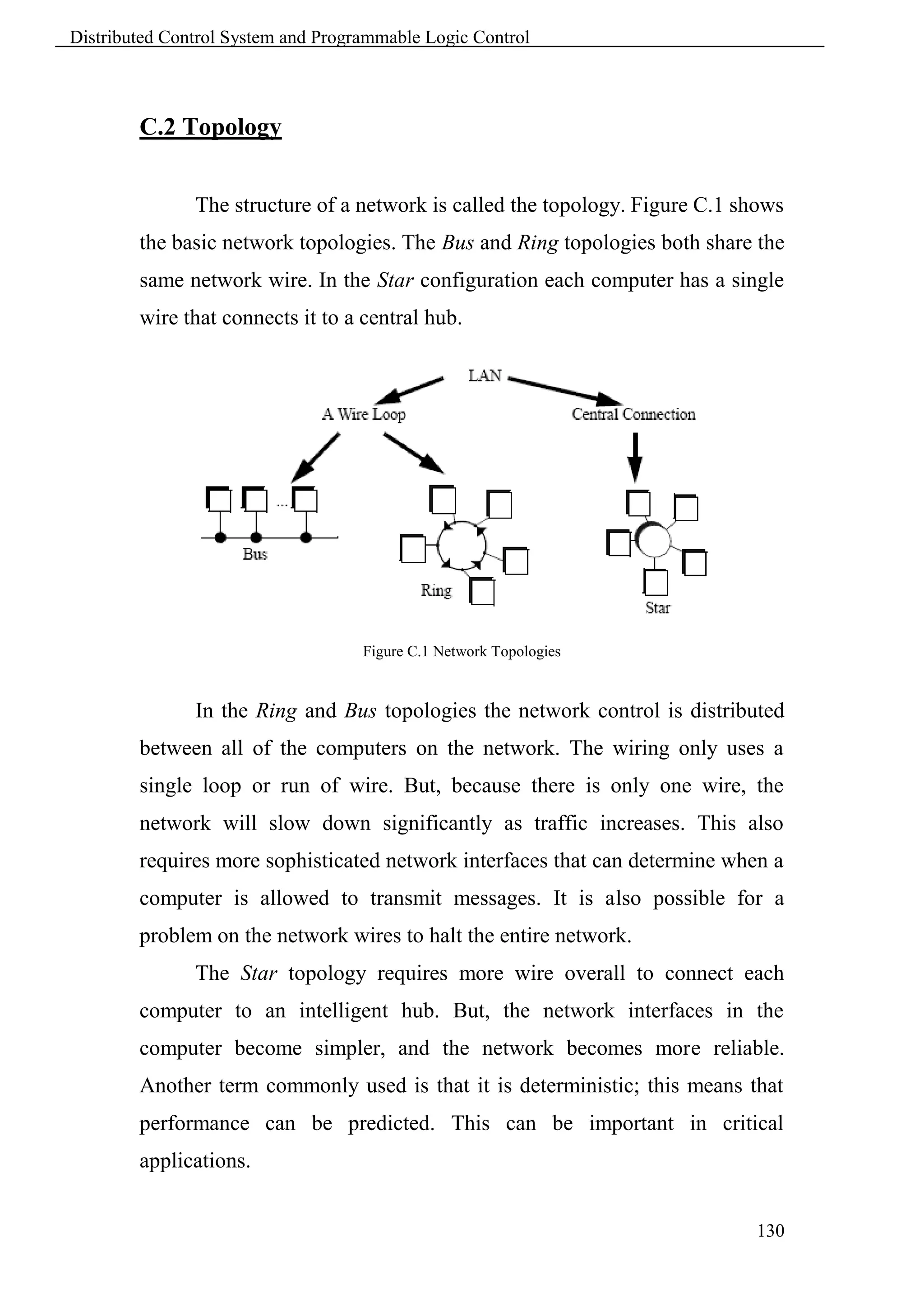
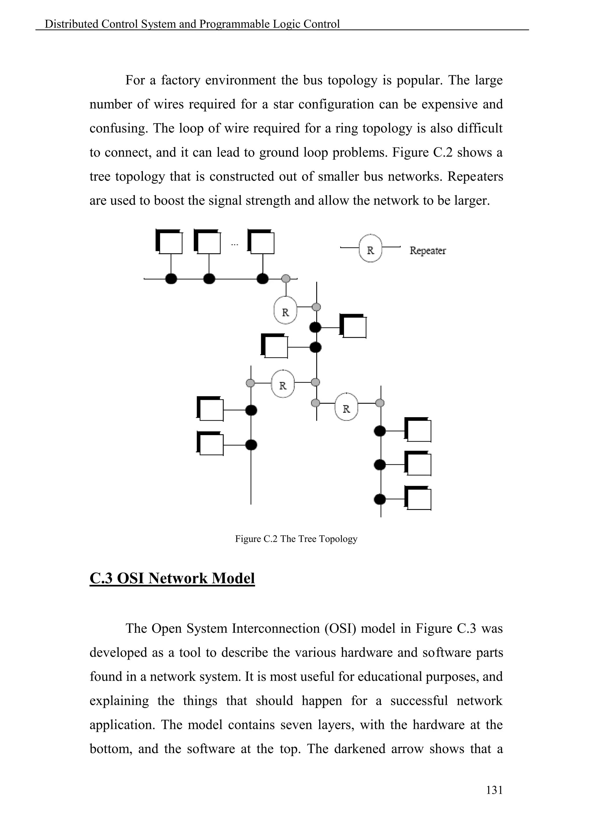
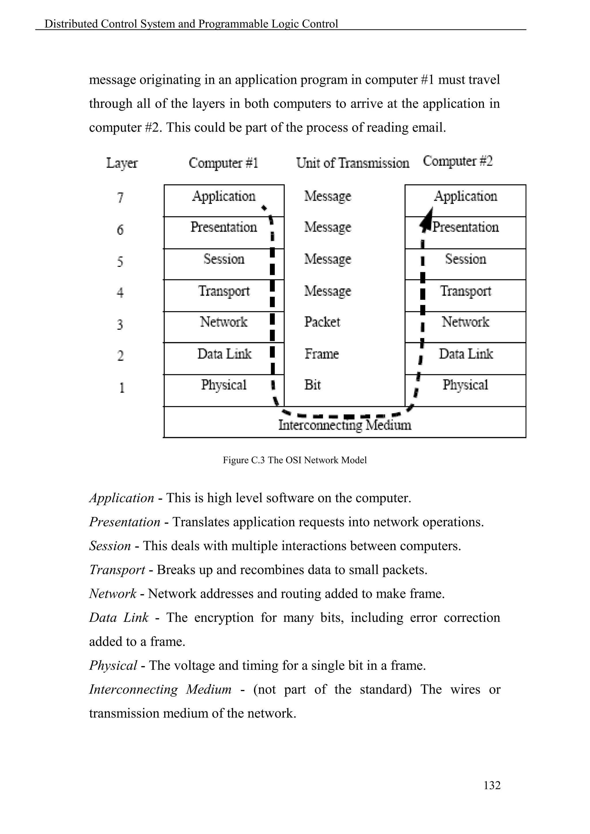

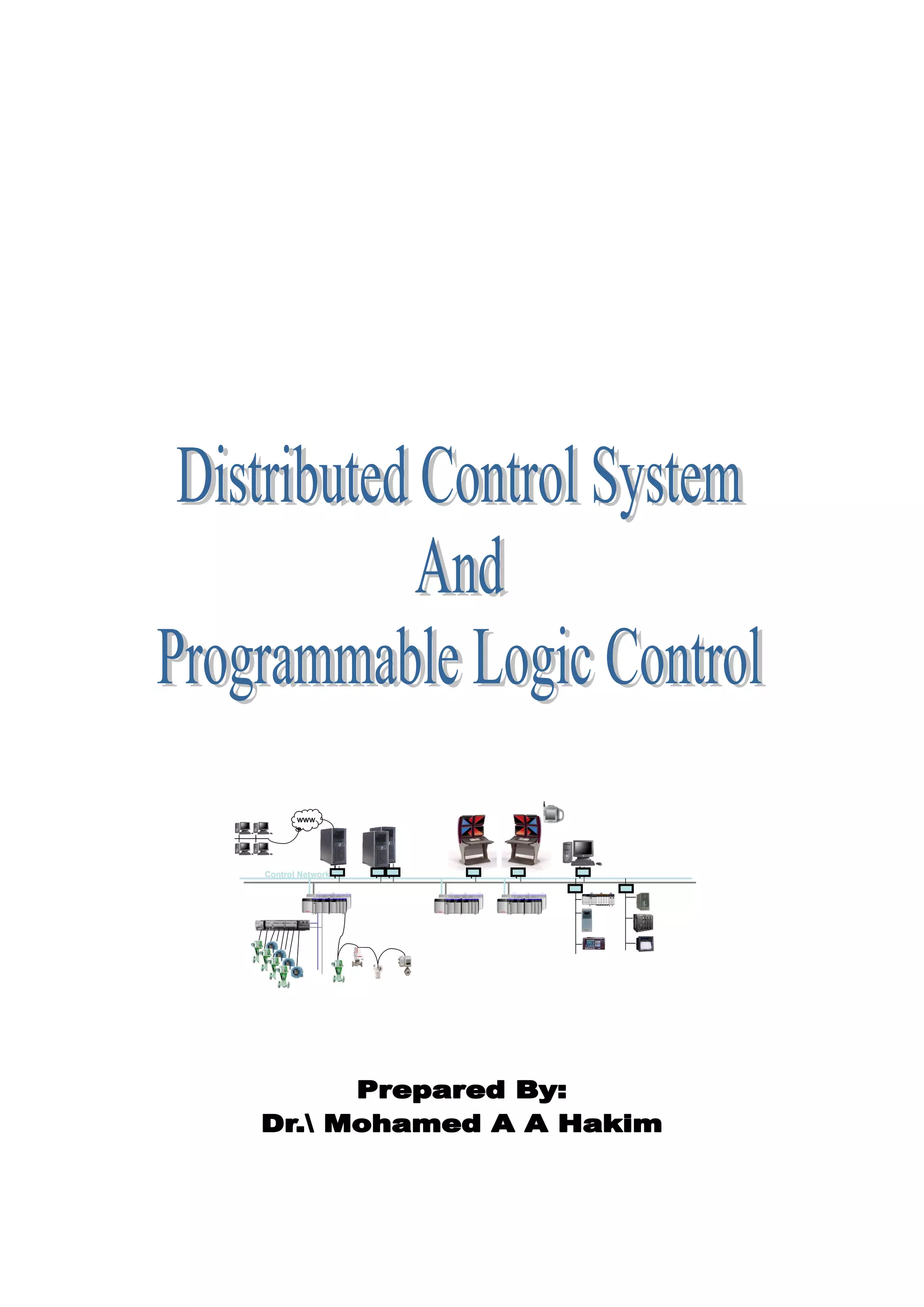
This document provides an overview of distributed control systems (DCS) and programmable logic controllers (PLC). It defines DCS and PLCs, compares them, and describes their basic components and functions. The key aspects covered are: 1) DCS are integrated control systems used for complex, large-scale processes, while PLCs are used for discrete and small-scale control. 2) Both have centralized processing units and input/output modules to interface with field devices. 3) DCS are designed for continuous long-term use, while PLCs are more modular project-based systems.