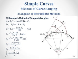
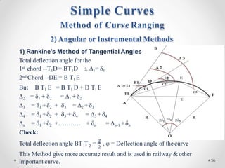
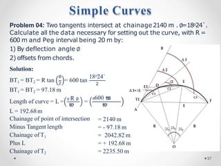
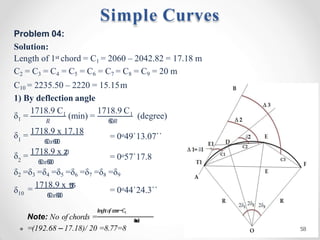
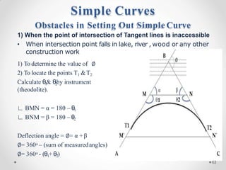
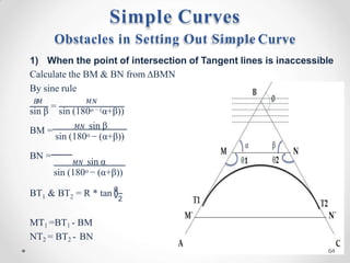
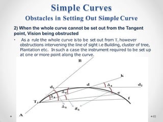
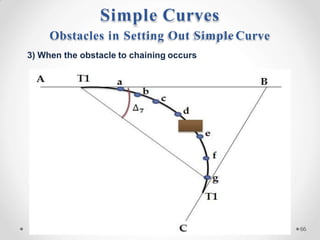
Download to read offline
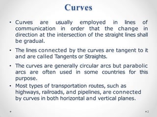
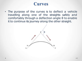
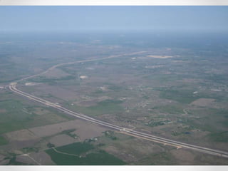


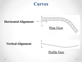
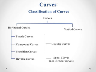
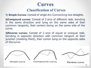
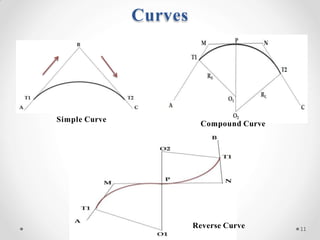
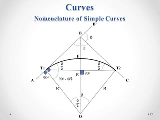
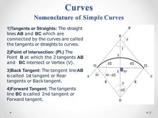
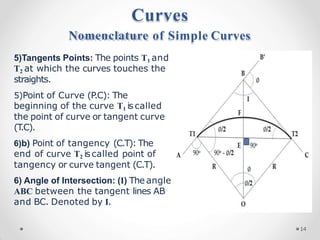
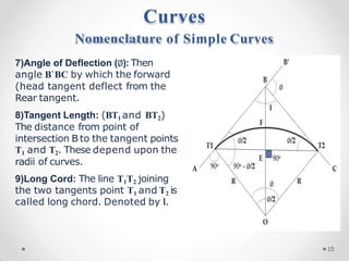
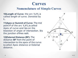
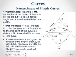
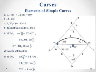
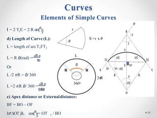
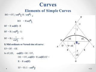
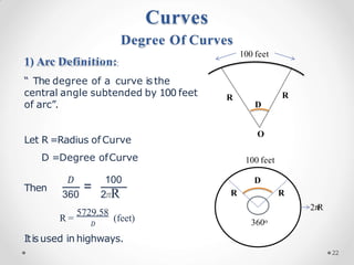
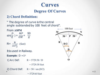
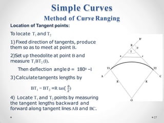
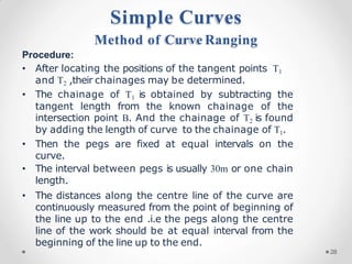
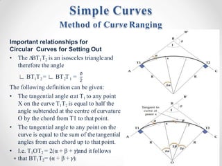
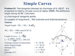
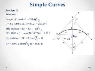
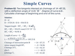
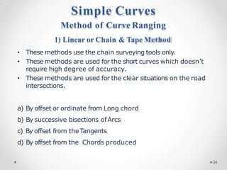
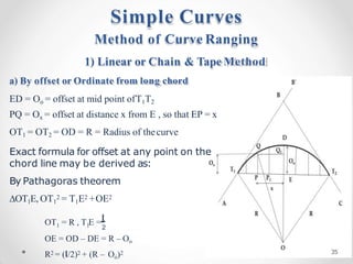
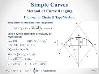
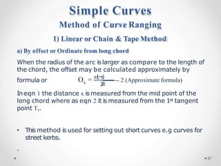
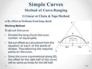
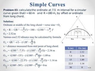
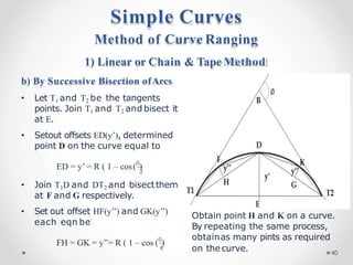
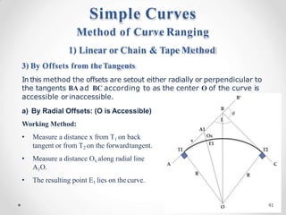
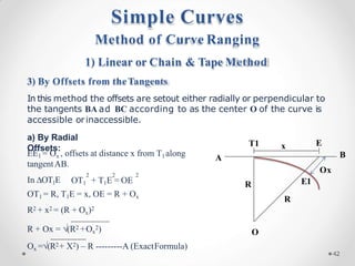
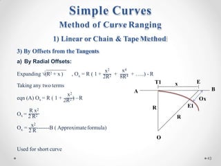
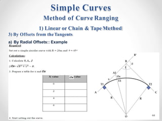
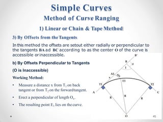
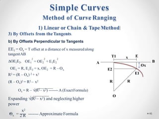
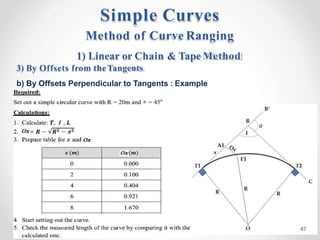
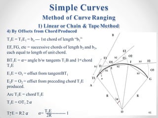
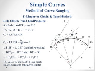
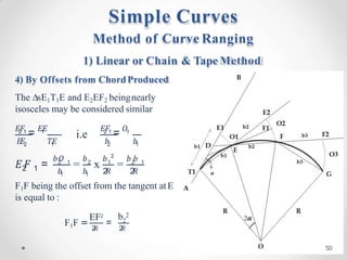
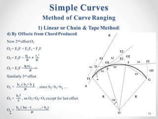
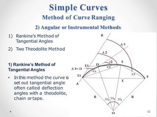
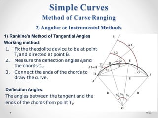
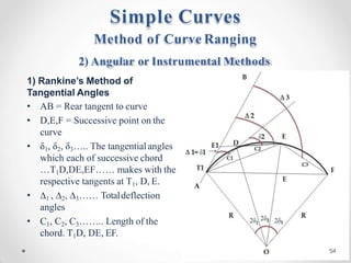
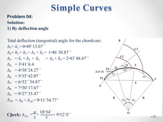
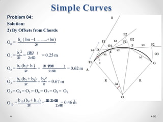
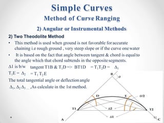
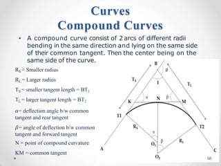
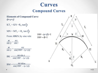
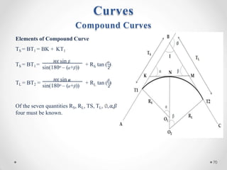
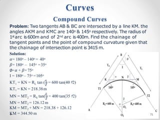
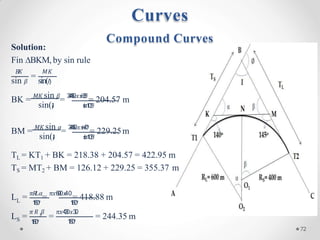
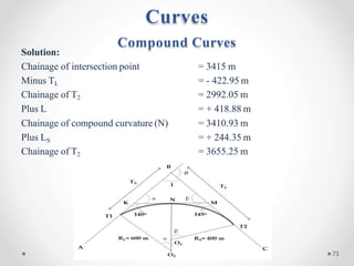

This document discusses curves used in transportation routes. It defines different types of curves including simple, compound, and reverse curves. It provides the nomenclature and key elements of simple circular curves, such as tangents, points of intersection and tangency, deflection angle, chord length, arc length, and mid-ordinate. The document also discusses the designation and degree of curves, and describes methods for setting out curves using linear measurements or angular measurements along the curve. Sample problems are provided to demonstrate how to calculate elements of a simple circular curve given radius, deflection angle, and chainage information.


