![Computing a Vertical Curve
Procedures for computing a vertical curve:
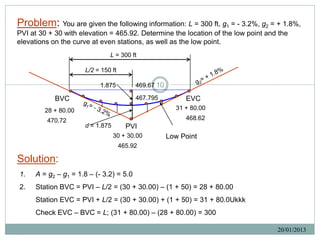
1. Compute the algebraic difference in grades A = g1 – g2.
2. Compute the stationing of BVC and EVC. Subtract/add L/2 to the PVI.
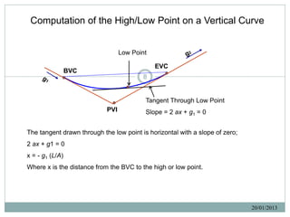
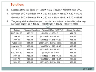
3. Compute the distance from the BVC to the high or low point; x = - g1(L/A). Determine
the station of the high or low point. 9
4. Compute the tangent gradeline elevation of the BVC and the EVC.
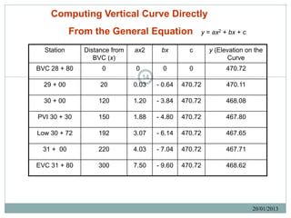
5. Compute the tangent gradeline elevation for each required station.
6. Compute the midpoint of the chord elevation: [(elevation of BVC + elevation of EVC)/2].
7. Compute the tangent offset d at PVI, Vm, d = (difference in elevation of PVI and C)/2).
8. Compute the tangent offset for each individual station (see line ax2),
tangent offset = d (x)2/(L/2)2 = (4d) x2/L2 where x is the distance from the BVC or EVC
(whichever is closer) to the required station.
9. Compute the elevation on the curve at each required station by combining the tangent
offsets with the appropriate tangent gradeline elevations. Add for sag curves and
subtract for crest curves.
20/01/2013](https://image.slidesharecdn.com/verticalcurves-130119170301-phpapp02/85/Vertical-Curves-Part-1-9-320.jpg)
![Solution:
6. Mid-chord elevation; [470.72 (BVC) + 468.62 (EVC)]/2 = 469.67 ft.
7. Tangent offset at PVI (d): d = (difference in elevation of PVI and mid-chord)/2
d = (469.67 – 465.92)/2 = 1.875 ft.
8. For other stations, tangent offsets are computed by multiplying the distance ratio
squared (x/L/2)2 by the maximum tangent offset (d). Refer to previous Table.
9. 12
The computed tangent offsets are added to the tangent elevation to determine the
curve elevation.
20/01/2013](https://image.slidesharecdn.com/verticalcurves-130119170301-phpapp02/85/Vertical-Curves-Part-1-12-320.jpg)
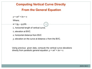

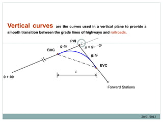
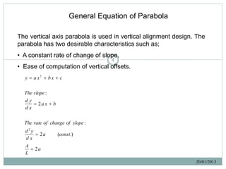
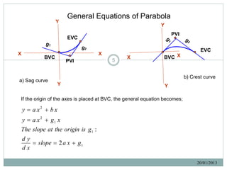
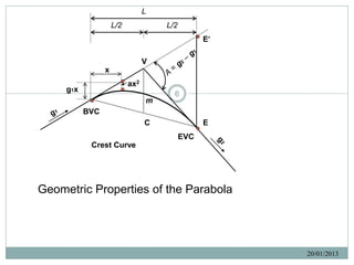
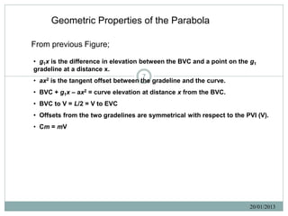
This document discusses vertical curves used in transportation design. Vertical curves provide a smooth transition between different road or rail grades. They are designed using parabolic equations to maintain a constant rate of change in slope. The key points are: - Vertical curves connect two different grades using a parabolic shape. - Their design ensures a constant rate of change in slope for driver comfort. - The general parabolic equation and methods for computing curve elements like high/low points and elevations at different points are presented.


![Geotechnical Engineering-I [Lec #21: Consolidation Problems]](https://cdn.slidesharecdn.com/ss_thumbnails/21-180924141121-thumbnail.jpg?width=640&height=640&fit=bounds)


