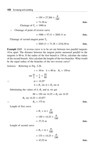
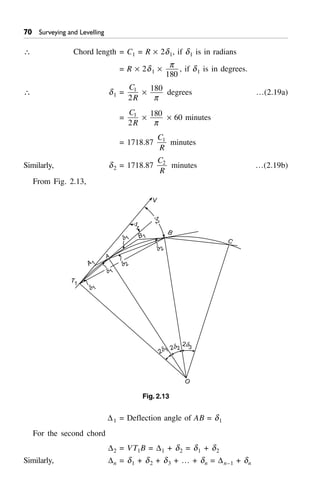
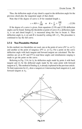
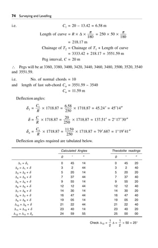
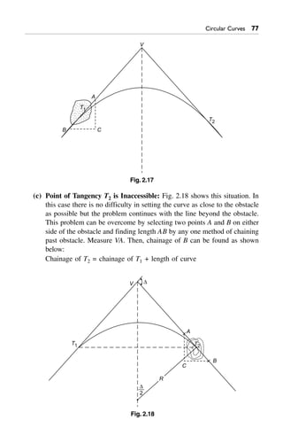
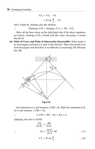
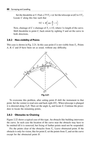
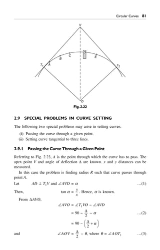
The document discusses circular curves as essential components in road and railway design, focusing on their types (horizontal and vertical) and characteristics such as radius, degree of curvature, and various elements like chord length and tangent distance. It provides methods for setting out these curves, including linear and angular methods, and details calculations using arc and chord definitions to determine curve parameters. Additionally, examples illustrate practical applications in engineering contexts.

1. Circular Curves #
Whenever the direction of a road or railway line is to be changed, curves are
provided between the intersecting straights. This is necessary for smooth and safe
movement of the vehicles and for the comfort of passengers. The curves required
may be in the horizontal planes or in the vertical planes. Accordingly the curves
are classified as horizontal curves and vertical curves.
Horizontal curves are further classified as circular curves and transition
curves.
Circular Curves
+ 0 ) 2 6 - 4
T1
T2
O
V
T2
T1
T
V
O1
O2
R R
R1
R2
(b)(a)
O2
T2
O1
T1 u
T
v
R1
R2
(c)
Fig. 2.1 Circular Curves

2. 54 Surveying and Levelling
11. Long Chord (L): The chord of the circular curve T1T2 is known as long
chord and is denoted by L.
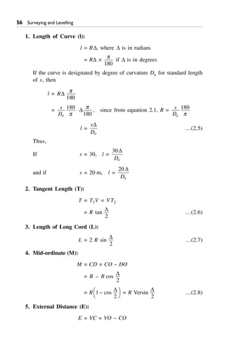
12. Length of Curve (l): The curved length T1CT2 is called the length of
curve.
13. Tangent Distance (T): The tangent distance is the distance of tangent
points T1 or T2 from vertex V. Thus,
T = T1V = VT2
14. Mid ordinate: It is the distance between the mid-point of the long chord
(D) and mid point of the curve (C). i.e.
Mid ordinate = DC
15. External Distance (E): It is the distance between the middle of the curve
to the vertex. Thus,
E = CV
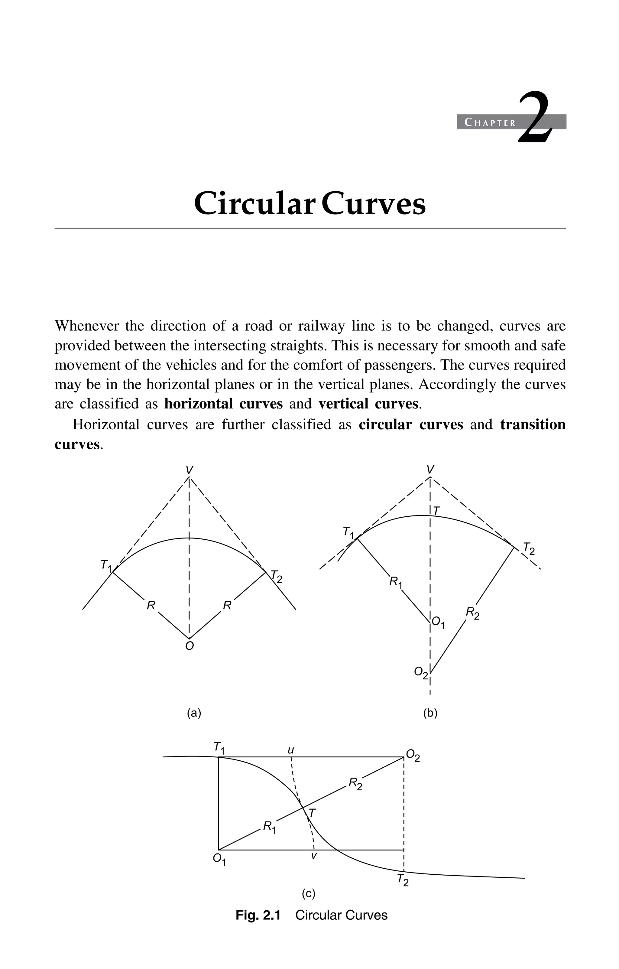
2.2 DESIGNATION OF A CURVE
In Great Britain the sharpness of the curve is designated by the radius of the curve
while in India and many countries it is designated by the degree of curvature.
There are two different definitions of degree of curvature:
(i) Arc Definition
(ii) Chord Definition.
According to arc definition degree of curvature is defined as angle in degrees
subtended by an arc of standard length [Fig. 2.4(a)]. This definition is generally
used in highway practice. The length of standard arc used in FPS was 100 ft. In
SI it is taken as 30 m. Some people take it as 20 m also.
Standard length
O
D°
O
D°
Standard length
(a) Arc Definition (b) Chord Definition
Fig. 2.4 Designation of a Curve
According to chord definition degree of curvature is defined as angle in degrees
subtended by a chord of standard length [Fig. 2.4(b)]. This definition is com-

3. Circular Curves 55
monly used in railways. Earlier standard chord length used was 100 ft. Now in
SI 30 m or 20 m is used as standard chord length.
2.3 RELATIONSHIP BETWEEN RADIUS AND
DEGREE OF CURVE
(a) Arc Definition:
Let – R be the radius
– s be standard length
– Da be degree of the curve
Referring to Fig. 2.4(a)
s = R ¥ Da ¥
p
180
or R = s
Da
¥
180
p
…(2.1)
If s = 20 m,
R = 20
Da
¥
180
p
= 1145 92.
Da
…(2.2a)
If s = 30 m,
R = 30
Da
¥
180
p
= 171887.
Da
…(2.2b)
(b) Chord Definition: Let Dc be degree of curve as per chord definition and
s be the standard length of chord. Then referring to Fig. 2.4(b).
R sin
Dc
2
=
s
2
…(2.3)
When Dc is small, sin
Dc
2
may be taken approximately equal to
Dc
2
radians.
Hence, for small degree curves (flat curves).
R
Dc
2
¥
p
180
=
s
2
or R = s
Dc
¥
180
p
…(2.4)
Comparing equations (2.1) and (2.4), we find for flat curves, arc defi-
nition and chord definitions give same degree of curve. As in railways flat
curves are used, chord definition is preferred.
2.4 ELEMENTS OF SIMPLE CURVES
Referring to Fig. 2.3, in which R is radius of the curve and D is deflection angle,
the formulae for finding various elements of curve can be derived as under:

4. #$ Surveying and Levelling
1. Length of Curve (l):
l = RD, where D is in radians
= RD ¥
p
180
if D is in degrees
If the curve is designated by degree of curvature Da for standard length
of s, then
l = RD
p
180
= s
Da
180
p
◊ D
p
180
, since from equation 2.1, R = s
Da
180
p
l =
s
Da
D
…(2.5)
Thus,
If s = 30, l =
30D
Da
and if s = 20 m, l =
20 D
Da
2. Tangent Length (T):
T = T1V = VT2
= R tan
D
2
…(2.6)
3. Length of Long Cord (L):
L = 2 R sin
D
2
…(2.7)
4. Mid-ordinate (M):
M = CD = CO – DO
= R – R cos
D
2
= R 1
2
-FH IKcos
D
= R Versin
D
2
…(2.8)
5. External Distance (E):
E = VC = VO – CO

5. Circular Curves #%
= R sec
D
2
– R
= R sec
D
2
1-FH IK = R exsec
D
2
…(2.9)
Example 2.1 A circular curve has 300 m radius and 60° deflection angle. What
is its degree by (a) arc definition and (b) chord definition of standard length 30 m.
Also calculate (i) length of curve, (ii) tangent length, (iii) length of long chord, (iv)
mid-ordinate and (v) apex distance.
Solution:
R = 300 m D = 60°
(a) Arc definition:
s = 30 m,
R = s
Da
¥
180
p
300 =
30 180¥
Da p
or Da = 5.730 Ans.
(b) Chord definition:
R sin
Dc
2
=
s
2
300 sin
Dc
2
=
30
2
DC = 5.732 Ans.
(i) Length of the curve:
l = RD
p
180
= 300 ¥ 60 ¥
p
180
= 314.16 m Ans.
(ii) Tangent length:
T = R tan
D
2
= 300 tan
60
2
= 173.21 m Ans.
(iii) Length of long chord:
L = 2 R sin
D
2
= 2 ¥ 300 ¥ sin
60
2
= 300 m Ans.
(iv) Mid-ordinate:
M = R 1
2
-FH IKcos
D = 300 1
60
2
-FH IKcos = 40.19 m Ans.

6. 58 Surveying and Levelling
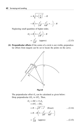
(v) Apex distance:
E = R sec
D
2
1-FH IK = 300 sec
60
2
1-FH IK = 46.41 m Ans.
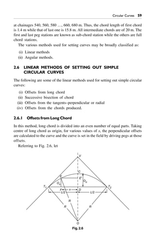
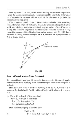
2.5 SETTING OUT A SIMPLE CIRCULAR CURVE
After aligning the road/railway along AA¢, when curve is to be inserted, alignment
of B¢B is laid on the field by carefully going through the alignment map and field
notes [Fig. 2.5].
T1 T21
2
3
4 5 6
7
8
9
A
A¢
A
B¢
B
D
2
D
2
O
Fig. 2.5
By ranging from AA¢ and BB¢, the vertex point V is determined. Setting a
theodolite at V, the deflection angle is measured carefully. The tangent distance T1
is calculated. Subtracting this value from chainage of V, chainage of point of curve
T1 is found. Adding length of curve to this chainage of T2 can be easily found.
Now pegs are to be fixed along the required curve at suitable intervals. It is
impossible to measure along the curve. Hence, for fixing curve, chord lengths are
taken as curved length. Chord length for peg interval is kept
1
10
th to
1
20
th of
radius of curve. When it is
1
10
th of R, the error is 1 in 2500 and if it is
1
20
th R,
the error is 1 in 10,000. In practice the radius of the curve varies from 200 m to
1000 m. Hence, the chord length of 20 m is reasonably sufficient. For greater
accuracy it may be taken as 10 m.
In practice, pegs are fixed at full chain distances. For example, if 20 m chain
is used, chainage of T1 is 521.4 m and that of T2 is 695.8 m, the pegs are fixed

7. Circular Curves 59
at chainages 540, 560, 580 …, 660, 680 m. Thus, the chord length of first chord
is 1.4 m while that of last one is 15.8 m. All intermediate chords are of 20 m. The
first and last peg stations are known as sub-chord station while the others are full
chord stations.
The various methods used for setting curves may be broadly classified as:
(i) Linear methods
(ii) Angular methods.
2.6 LINEAR METHODS OF SETTING OUT SIMPLE
CIRCULAR CURVES
The following are some of the linear methods used for setting out simple circular
curves:
(i) Offsets from long chord
(ii) Successive bisection of chord
(iii) Offsets from the tangents–perpendicular or radial
(iv) Offsets from the chords produced.
2.6.1 Offsets from Long Chord
In this method, long chord is divided into an even number of equal parts. Taking
centre of long chord as origin, for various values of x, the perpendicular offsets
are calculated to the curve and the curve is set in the field by driving pegs at those
offsets.
Referring to Fig. 2.6, let
D
E
F
C
V
T1
Ox
Oo
E¢
T2
L/2 L/2
x
R R
R
O
Fig. 2.6

8. 60 Surveying and Levelling
R – radius of the curve
L – length of long chord
O0 – mid-ordinate
Ox – ordinate at distance x from the mid-point of long chord
Ordinate at distance x = Ox = E¢O – DO
= R x R L2 2 2 2
2- - - ( / ) …(2.10)
The above expression holds good for x-values on either side of D, since CD
is symmetric axis.
2.6.2 Successive Bisection of Chords
In this method, points on a curve are located by bisecting the chords and erecting
the perpendiculars at the mid-point.
Referring to Fig. 2.7
T1 T2
C2
C1
C2
C2
C1
C2
D 1 D1
D
O
C
R R
D 2
D 2 D2
D2
Fig. 2.7
Perpendicular offset at middle of long chord (D) is
CD = R – R cos
D
2
= R 1
2
-FH IKcos
D
…(2.11a)

9. Circular Curves 61
Let D1 be the middle of T1C. Then Perpendicular offset
C1D1 = R 1
4
-FH IKcos
D
…(2.11b)
Similarly, C2D2 = R 1
8
-FH IKcos D …(2.11c)
Using symmetry points on either side may be set.
2.6.3 Offsets from the Tangents
The offsets from tangents may be calculated and set to get the required curve.
The offsets can be either radial or perpendicular to tangents.
(i) Radial offsets: Referring to Fig. 2.8, if the centre of curve O is accessible
from the points on tangent, this method of curve setting is possible.
O
C
E
T1
Ox
D
x
R
R
Fig. 2.8
Let D be a point at distance x from T1. Now it is required to find radial
ordinate Ox = DE, so that the point C on the curve is located.
From D OT1D, we get
OD2
= OT1
2
+ T1D2
(R + Ox)2
= R2
+ x2
i.e. Ox + R = R x2 2
+
or Ox = R x2 2
+ – R …(2.12)
An approximate expression Ox may be obtained as explained below:
Ox = R x2 2
+ – R

10. $ Surveying and Levelling
= R
x
R
1
2
+ FH IK – R
ª R 1
2 8
2
2
2
4
+ - + º
F
HG I
KJx
R
x
R
– R
Neglecting small quantities of higher order,
Ox = R 1
2
2
2
+
F
HG I
KJx
R
– R
= x
R
2
2
2
(approx) …(2.13)
(ii) Perpendicular offsets: If the centre of a circle is not visible, perpendicu-
lar offsets from tangent can be set to locate the points on the curve.
E1
E
C
D
x
Ox
V
O
T1
Fig. 2.9
The perpendicular offset Ox can be calculated as given below:
Drop perpendicular EE1 to OT1. Then,
Ox = DE = T1 E1
= OT1 – OE1
= R – R x2 2
- (Exact) …(2.14)
= R – R 1
2 8
2
2
4
4
- - º
F
HG I
KJx
R
x
R
=
x
R
2
2 (approx) …(2.15)

11. Circular Curves 63
From equations (2.13) and (2.15) it is clear that they are equations for parabola.
Hence, the approximation is circular curve is replaced by a parabola. If the versed
sin of the curve is less than 1/8th of its chord, the difference in parabola and
circular curve is negligible.
If the exact equations (2.12) and (2.14) are used, the circular curve is correctly
found. However, when offsets become longer, the errors in setting offsets creep
in. Hence, it is better to find the additional tangents and set offsets, if the curve
is long. The additional tangent at C can be easily set, because it is parallel to long
chord. One can even think of finding intermediate tangents also. Fig. 2.10 shows
a scheme of finding additional tangent NK at K, in which NL is perpendicular to
T1K at its mid-point L.
M
N
L
T1
K
Additional Tangent
Ox¢
Fig. 2.10
2.6.4 Offsets from the Chord Produced
This method is very much useful for setting long curves. In this method, a point
on the curve is fixed by taking offset from the tangent taken at the rear point of
a chord.
Thus, point A of chord T1A is fixed by taking offset O1 = AA1 where T1A1 is
tangent at T1. Similarly B is fixed by taking offset O2 = BB1 where AB1 is tangent
at A.
Let T1A = C1 be length of first sub-chord
AB = C2 be length of full chord
d1 = deflection angle A1T1A
d2 = deflection angle B1AB
Then from the property of circular curve
T1OA = 2d1
C1 = chord T1A ª Arc T1A = R 2d1

12. $ Surveying and Levelling
i.e. d1 =
C
R
1
2
…(i)
Now, offset O1 = arc AA1
= C1d1 …(ii)
Substituting the value of d1 from equation (i) into equation (ii), we get
O1 = C1 ¥
C
R
1
2
=
C
R
1
2
2
…(2.16)
From Fig. 2.11,
B C
C= 2
3
B1
V
T1
C1
A2
A1
C2
d
1
d
1
d
2
d
2
d1
2d
1
2d 2
2d2
O
O2
B
2
O1
A
Fig. 2.11
O2 = C2 (d1 + d2)
= C2
C
R
C
R
1 2
2 2
+
F
HG I
KJ
=
C
R
2
2
(C1 + C2) …(2.17)
Similarly, O3 =
C
R
3
2
(C2 + C3)
But, C3 = C2 O3 =
C
R
2
2

13. Circular Curves 65
Thus, upto last full chord i.e. n – 1 the chord,
On–1 =
C
R
2
2
2
If last sub-chord has length Cn, then,
On =
C
R
n
2
(Cn–1 + Cn) …(2.18)
Note that Cn–1 is full chord.
Procedure for Setting the Curve
1. Locate the tangent points T1 and T2 and find the length of first (C1) and
last (Cn) sub-chord, after selecting length (C2 = C3…) of normal chord
[Ref Art 2.5].
2. Stretch the chain or tape along T1V direction, holding its zero end at T1.
3. Swing the arc of length C1 from A1 such that A1A =
C
R
1
2
2
. Locate A.
4. Now stretch the chain along T1AB1. With zero end of tape at A, swing the
arc of length C2 from B1 till B1B = O2 =
C C C
R
2 1 2
2
( )+
. Locate B.
5. Spread the chain along AB and the third point C such that C2 O3 =
C
R
2
2
at
a distance C3 = C2 from B. Continue till last but one point is fixed.
6. Fix the last point such that offset On =
C C C
R
n2 2
2
( )+
.
7. Check whether the last point coincides with T2. If the closing error is large
check all the measurements again. If small, the closing error is distributed
proportional to the square of their distances from T1.
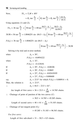
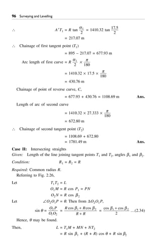
Example 2.2 Two roads having a deviation angle of 45° at apex point V are to
be joined by a 200 m radius circular curve. If the chainage of apex point is
1839.2 m, calculate necessary data to set the curve by:
(a) ordinates from long chord at 10 m interval
(b) method of bisection to get every eighth point on curve
(c) radial and perpendicular offsets from every full station of 30 m along
tangent.
(d) offsets from chord produced.
Solution:
R = 200 m D = 45°

14. $$ Surveying and Levelling
Length of tangent = 200 tan
45
2
= 82.84 m.
Chainage of T1 = 1839.2 – 82.84 = 1756.36 m.
Length of curve = R ¥ 45 ¥
p
180
= 157.08 m
Chainage of forward tangent T2
= 1756.36 + 157.08 = 1913.44 m.
(a) By offsets from long chord:
45°V
C
T1
T2
6 5 4 3 2 1 1 2 3 4 5 6
D
45
2
45
2
O
Fig. 2.12
Distance of DT = L/2 = R sin
D
2
= 200 sin
45
2
= 76.54
Measuring ‘x’ from D,
y = R x R L2 2 2 2
2- - - ( / )
At x = 0
O0 = 200 – 200 76 542 2
- . = 200 – 184.78
= 15.22 m
O1 = 200 102 2
- – 184.78 = 14.97 m
O2 = 200 202 2
- – 184.78 = 14.22 m

15. Circular Curves $%
O3 = 200 302 2
- – 184.78 = 12.96 m
O4 = 200 402 2
- – 184.78 = 11.18 m
O5 = 200 502 2
- – 184.78 = 8.87 m
O6 = 200 602 2
- – 184.78 = 6.01 m
O7 = 200 702 2
- – 184.28 = 2.57 m
At T1, O = 0.00
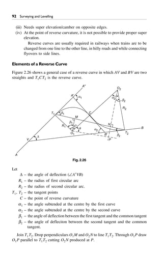
(b) Method of bisection: Referring Fig. 2.7,
Central ordinate at D = R 1
2
-FH IKcos
D
= 200 1
45
2
-FH IKcos
= 15.22
Ordinate at D1 = R 1
4
-FH IKcos
D = 200 1
45
4
-FH IKcos
= 3.84 m
Ordinate at D2 = R 1
8
-FH IKcos D = 200 1 45
8
-FH IKcos
= 0.96 m
(c) Offsets from tangents:
Radial offsets: [Fig. 2.8]
Ox = R x2 2
+ – R
Chainage of T1 = 1756.36 m
For 30 m chain, it is at
= 58 chains + 16.36 m.
x1 = 30 – 16.36 = 13.64
x2 = 43.64 m
x3 = 73.64 m
and the last is at x4 = tangent length = 82.84 m
O1 = 200 13 642 2
+ . – 200 = 0.46 m
O2 = 200 43 642 2
+ . – 200 = 4.71 m
O3 = 200 73642 2
+ . – 200 = 13.13 m
O4 = 200 82 842 2
+ . – 200 = 16.48 m

16. $ Surveying and Levelling
(d) Offsets from chord produced:
Length of first sub-chord = 13.64 m = C1
Length of normal chord = 30 m = C2
Since length of chain is 157.08 m, C3 = C4 = C5 = 30 m
Chainage of forward tangent = 1913.44 m
= 63 chains + 23.44 m
Length of last chord = 23.44 m = Cn = C6
O1 =
C
R
1
2
2
=
13 64
2 200
2
.
¥
= 0.47 m
O2 =
C C C
R
2 1 2
2
( )+
=
30 30 13 64
2 200
( . )+
¥
= 3.27 m
O3 =
C
R
2
2
=
30
2 200
2
¥
= 4.5 m = O4 = O5
O6 =
C C C
R
n n n( )- +1
2
=
23 44 23 44 30
2 200
. ( . )+
¥
= 3.13 m
Example 2.3 Two tangents intersect at the chainage 1190 m, the deflection
angle being 36°. Calculate all the data necessary for setting out a circular curve
with radius of 300 m by deflection angle method. The peg interval is 30 m.
Solution:
Chainage of apex V = 1190 m
Deflection angle D = 36°
Radius R = 300 m
Peg interval = 30 m.
Length of tangent = R tan
D
2
= 300 tan
36
2
= 97.48 m
Chainage of T1 = 1190 – 97.48 = 1092.52 m
= 36 chains + 12.52 m
C1 = 30 – 12.52 = 17.48 m
C2 = 30
Length of curve = R ¥ D ¥
p
180
= 300 ¥ 36 ¥
p
180
= 188.50 m
C3 = C4 = C5 = C6 = 30 m
Cn = C7 = 188.5 – 17.48 – 30 ¥ 5 = 21.02 m
Chainage of T2 = 1092.52 + 188.50 = 1281.02 m

17. Circular Curves 69
Ordinates are
O1 =
C
R
1
2
2
=
17 48
2 300
2
.
¥
= 0.51 m
O2 =
C C C
R
2 2 1
2
( )+
¥
=
30 30 17 48
2 300
( . )+
¥
= 2.37 m
O3 = O4 = O5 = O6 = 30
300
2
= 3.0 m
O7 =
2102 2102 30
2 300
. ( . )+
¥
= 1.79 m
2.7 ANGULAR METHOD (INSTRUMENTAL METHOD)
The following are the angular methods which can be used for setting circular
curves:
(i) Rankine method of tangential (deflection) angles.
(ii) Two-theodolite method
(iii) Tacheometric method
In these methods linear as well as angular measurements are used. Hence, the
surveyor needs chain/tape and instruments to measure angles. Theodolite is the
commonly used instrument. These methods are briefly explained in this chapter.
2.7.1 Rankine’s Method of Tangential (or Deflection) Angles
A deflection angle to any point on the curve is the angle between the tangent at
point of curve (PC) and the line joining that point to PC (D). Thus, referring to
Fig. 2.13, d1 is the deflection angle of A and d1 + d2 is the deflection angle of B.
In this method points on the curve are located by deflection angles and the
chord lengths. The formula for calculating deflection angles of various chords can
be derived as shown below:
Let A, B, C … be points on the curve. The chord lengths T1A, AB, BC… be
C1, C2, C3… and d1, d2, d3… tangential angles, which of the successive chords
make with respective tangents. D1, D2, D3… be deflection angles.
–VA1A = –A1T1A + –A1AT1 = d1 + d1
= 2d1
From the property of circular curve,
–T1OA = –VA1A = 2d1

18. % Surveying and Levelling
Chord length = C1 = R ¥ 2d1, if d1 is in radians
= R ¥ 2d1 ¥
p
180
, if d1 is in degrees.
d1 =
C
R
1
2
¥
180
p
degrees …(2.19a)
=
C
R
1
2
¥
180
p
¥ 60 minutes
= 1718.87
C
R
1
minutes
Similarly, d2 = 1718.87
C
R
2
minutes …(2.19b)
From Fig. 2.13,
B
A
T1
A 1
d 1
d 2
d 1
2d 1
O
B 1
2d2
2d3
C
D
1
d 1
d 2
D2
V
Fig. 2.13
D1 = Deflection angle of AB = d1
For the second chord
D2 = VT1B = D1 + d2 = d1 + d2
Similarly, Dn = d1 + d2 + d3 + … + dn = Dn–1 + dn

19. Circular Curves 71
Thus, the deflection angle of any chord is equal to the deflection angle for the
previous chord plus the tangential angle of that chord.
Note that if the degree of curve is D for standard length s,
s = RD ¥
p
180
or R =
s
D
¥
180
p
…(2.20)
If the degree of a curve is given, from equations (2.19) and (2.20) deflection
angles can be found. Setting the theodolite at point of curve (T1), deflection angle
D1 is set and chord length C1 is measured along this line to locate A. Then
deflection angle D2 is set and B is located by setting AB = C2. The procedure is
continued to lay the full curve.
2.7.2 Two-Theodolite Method
In this method, two theodolites are used, one at the point of curve (PC i.e. at T1)
and another at the point of tangency (PT i.e. at T2). For a point on the curve
deflection angle with back tangent and forward tangent are calculated. The the-
odolites are set at PC and PT to read these angles and simultaneous ranging is
made to get the point on the curve.
Referring to Fig. 2.14, let D1 be deflection angle made by point A with back
tangent and D¢1 be the deflected angle made by the same point with forward
tangent at T2. The method of finding D1 is already explained in the previous article.
To find expression for D¢1, draw a tangent at A intersecting back tangent at A1 and
forward tangent at A2.
T1 T2
A2
A1
D1
D1
A
D¢1
D¢1
D/2 D/2
V D
V¢
Fig. 2.14

20. 72 Surveying and Levelling
In triangle A1T1A, since A1T1 and A1A both are tangents,
–A1T1A = –A1AT1 = D1
Exterior angle VA1A2 = 2D1
Similarly, referring to triangle A2 AT2, we get
Exterior angle VA2A1 = 2D¢1
Now, considering the triangle VA1A2, the exterior angle
V¢ VA2 = –VA1A2 + –VA2A1
i.e. D = 2D1 + 2D¢1
D¢1 =
D
2
– D1 …(2.20)
Hence, after finding the deflection angle with back tangent (D1), the deflection
angle D¢1 with forward tangent can be determined.
Procedure to Set Out Curve
The following procedure is to be followed:
1. Set the instrument at point of curve T1, clamp horizontal plates at zero
reading and sight V. Clamp the lower plate.
2. Set another instrument at point of forward tangent T2, clamp the horizontal
plates at zero reading and sight V. Clamp the lower plate.
3. Set horizontal angles D1 and D¢1 in the theodolites at T1 and T2 and locate
intersecting point by ranging. Mark the point.
4. Similarly fix other points.
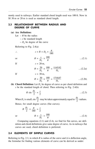
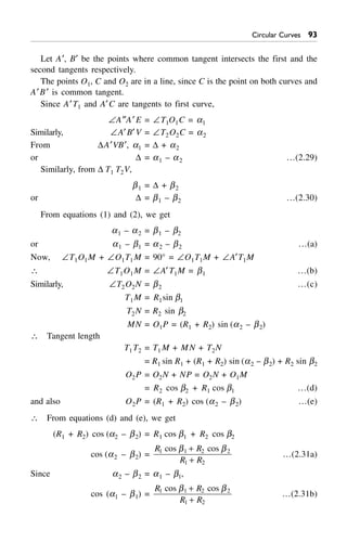
2.7.3 Tacheometric Method [Fig. 2.15]
If the terrain is rough, linear measurements may be replaced by the tacheometric
measurements. The lengths of chord T1A, T1 B … may be calculated from the
formula 2R sin D1, 2R sin D2 … etc. Then the respective staff intercepts s1, s2,
… may be calculated from the formula.
D =
f
i
s cos2
q + (f + d) cos q
= ks cos2
q + C cos q
Procedure to set the curve
1. Set the theodolite at T1.
2. With vernier reading zero sight the signal at V and clamp the lower plate.

21. % Surveying and Levelling
i.e. C1 = 20 – 13.42 = 6.58 m
Length of curve = R ¥ D ¥
p
180
= 250 ¥ 50 ¥
p
180
= 218.17 m
Chainage of T2 = Chainage of T1 + Length of curve
= 3333.42 + 218.17 = 3551.59 m
Peg interval, C = 20 m
Pegs will be at 3360, 3380, 3400, 3420, 3440, 3460, 3480, 3500, 3520, 3540
and 3551.59.
i.e. No. of normal chords = 10
and length of last sub-chord Cn = 3551.59 – 3540
Cn = 11.59 m
Deflection angles:
d1 =
C
R
1
¥ 1718.87 =
6 58
250
.
¥ 1718.87 = 45.24¢ = 45¢14≤
d =
C
R
¥ 1718.87 =
20
250
¥ 1718.87 = 137.51¢ = 2°17¢30≤
dn =
C
R
n
¥ 1718.87 =
1159
250
.
¥ 1718.87 = 79¢.687 = 1°19¢41≤
Deflection angles required are tabulated below.
Calculated Angles Theodolite readings
0 ¢ ≤ 0 ¢ ≤
D1 = d1 0 45 14 0 45 20
D2 = D1 + d 3 2 44 3 2 40
D3 = D2 + d 5 20 14 5 20 20
D4 = D3 + d 7 37 44 7 37 40
D5 = D4 + d 9 55 14 9 55 20
D6 = D5 + d 12 12 44 12 12 40
D7 = D6 + d 14 30 14 14 30 20
D8 = D7 + d 16 47 44 16 47 40
D9 = D8 + d 19 05 14 19 05 20
D10 = D9 + d 21 22 44 21 22 40
D11 = D10 + d 23 40 14 23 40 20
D12 = D11 + dn 24 59 55 25 00 00
Check D12 =
1
2
D =
1
2
¥ 50 = 25°

22. Circular Curves 75
2.8 OBSTACLES IN SETTING OUT SIMPLE
CIRCULAR CURVES
Obstacles in setting out of curves may be classified as due to inaccessibility, due
to non-visibility and/or obstacles to chaining of some of the points.
2.8.1 Inaccessibility of Points
This type of obstacles can be further classified as inaccessibility of:
(a) Point of Intersection (PI)
(b) Point of Curve (PC)
(c) Point of Tangency (PT)
(d) Point of Curve and Point of Intersection (PC and PI).
(e) Point of Curve and Point of Tangency (PC and PT).
The method of overcoming these problems are presented below:
(a) Point of Intersection is Inaccessible: When the intersection point V falls
in a lake, river, wood or behind a building, there is no access to the point
V. Referring to Fig. 2.16, T1 and T2 be the tangent points and V the point
of intersection. It is required to determine the value of the deflection angle
D between the tangents and locate the tangent points T1 and T2.
A
B
T2T1
q1 q2
M N
D
2
D
2
O
R R
V D
Fig. 2.16
Procedure:
1. Select points M and N suitably on the tangents so that they are
intervisible and there is no problem for measuring MN.

23. Circular Curves %%
T1
V
A
T2
CB
Fig. 2.17
(c) Point of Tangency T2 is Inaccessible: Fig. 2.18 shows this situation. In
this case there is no difficulty in setting the curve as close to the obstacle
as possible but the problem continues with the line beyond the obstacle.
This problem can be overcome by selecting two points A and B on either
side of the obstacle and finding length AB by any one method of chaining
past obstacle. Measure VA. Then, chainage of B can be found as shown
below:
Chainage of T2 = chainage of T1 + length of curve
T1
A
B
C
D
2
V D
R
T2
Fig. 2.18

24. % Surveying and Levelling
AT2 = VT2 – VA
= R tan
D
2
– VA
AB is found by chaining past the obstacle.
Chainage of B = chainage of T2 + AB – AT2.
Since all the three terms on the right-hand side of the above equations
are known, chainage of B is found with this value surveying is carried
beyond B.
(d) Point of Curve and Point of Intersection Inaccessible: Select point A
on rear tangent such that it is clear of the obstacle. Then select point B on
forward tangent such that there is no difficulty in measuring AB. Measure
line AB.
A
A¢
T¢
C
a
a
q1
T1
q2 B
V u
O
Fig. 2.19
Set instrument at A and measure –VAB = q1. Shift the instrument to B,
set it and measure –VBA = q2.
–AVB = 180 – (q1 + q2) = D
Applying sine rule to DVAB,
VA
sin q 2
= AB
sin D
VA =
sin
sin
q 2
D
AB …(1)
V T1 = R sin
D
2
…(2)

25. 80 Surveying and Levelling
Set the theodolite at V. Find –TVT2 = f. Set the telescope at f/2 to VT1.
Locate C along this line such that
VC = R sec
D
2
1-FH IK
Now, chainage of C = chainage of T1 + l/2, where l is length of the curve.
Shift theodolite to point C, back orient by sighting V and set the curve in
both directions.
2.8.2 Non-visibility of Points
This case is shown in Fig. 2.21. In this case point E is not visible from T1. Points
A, B, C and D have been set as usual, without any difficulty.
T1
D4
A
B
C
D
D4
D5
E F
O
V
T2
Fig. 2.21
To overcome this problem, after setting point D shift the instrument to that
point. Set the vernier to read zero and back sight DT1. When telescope is plunged
it is directed along T1D. Then set the angle D5 and locate E. Continue the proce-
dure to locate the remaining points.
2.8.3 Obstacles to Chaining
Figure 2.22 shows a typical case of this type. An obstacle like building intervenes
the curve. In such case the location of the curve near the obstacle may have to
be omitted till it is removed, but fixing of further points need not be suspended.
Fix the points clear of the obstacles from T1. Leave obstructed point. If the
obstacle is only for vision, like for point E, set the points from T1 and set the curve
except for the obstructed point D.

26. Circular Curves 81
V
A
B
C E
T1 T2
D
O
Fig. 2.22
2.9 SPECIAL PROBLEMS IN CURVE SETTING
The following two special problems may arise in setting curves:
(i) Passing the curve through a given point.
(ii) Setting curve tangential to three lines.
2.9.1 Passing the Curve Through a Given Point
Referring to Fig. 2.23, A is the point through which the curve has to pass. The
apex point V and angle of deflection D are known. x and y distances can be
measured.
In this case the problem is finding radius R such that curve passes through
point A.
Let AD ^ T1V and –AVD = a …(1)
Then, tan a =
y
x
. Hence, a is known.
From DAVO,
–AVO = –T1VO – –AVD
= 90 –
D
2
– a …(2)
= 90 – D
2
+FH IKa
and –AOV =
D
2
– q, where q = –AOT1 …(3)

27. Surveying and Levelling
–OAV = 180 – –AVO – –AOV
= 180 – 90
2
- -FH IKD
a – D
2
-FH IKq
= 90 + a + q …(4)
Applying sine rule to D AVO, we get
sin
sin
–
–
OAV
AVO
=
VO
OA
sin ( )
sin
90
90
2
+ +
- +FH IKL
NM O
QP
a q
aD
=
R
R
sec D
2 = sec D
2
cos (a + q) =
cos
cos
D
D
2
2
+FH IKa
…(2.23)
In equation (4) a and D are known. Hence, from it ‘q’ can be found.
Draw AB || DT1. Then,
T1B = T1O – BO
= R – R cos q = R(1 – cos q) …(5)
V
A
T1 T2
q
D/2
O
C
x
D
y
f
D
aB
Fig. 2.23

28. Circular Curves 83
But from figure,
T1B = AD = y
From equation (6),
y = R(1 – cos q)
or R =
y
1 - cos q
…(2.24)
Since q is already found from equation (2.23), R can be found from equation
(2.24). Hence, the problem is solved.
2.9.2 Setting Curve Tangential to Three Lines
In this case the problem is apart from the curve being tangential at T1 and T2, it
has to be tangential at a given point A as shown in Fig. 2.24. Let –T1OA = a and
–T2OA = b.
T2
T1
B
A
D
D
V
b
2
a
2a
2
b
2
O
Fig. 2.24
Let tangential line at A intersect, the tangents T1V and T2V at points B and D
respectively. Then from the property of circular curve,
–T1OB = –BOA = a/2
–AOD = –BOT2 = b/2
BA = R tan a/2
and AD = R tan b/2

29. Surveying and Levelling
BA + AD = R (tan a/2 + tan b/2)
Let BD = BA + AD = d
Then, d = R (tan a/2 + tan b/2)
i.e. R = d
tan / tan /a b2 2+
…(2.25)
Since a, b and d are known, the required radius R of the curve can be found.
Knowing radius R and angle of deflection D, the required calculations for setting
curve can be made.
Example 2.5 Two straights AV and BV meet on the far end of a river. A simple
circular curve of radius 600 m is to be set out entirely on the near side of the river,
connecting the two straights. To overcome this obstruction, a point M was
selected on AI and another point N on the BI, both the points being on the near
bank of the river. The distance MN was found to be 100 m. –AMN = 165°36¢,
–BNM = 168°44¢. Calculate the distances along the straights from M and N to
the respective tangents points and also the length of the curve.
Solution: Referring to Fig. 2.16,
R = 600 m, q1 = 165°36¢ q2 = 168°44¢
MN = 100 m
In DVMN,
–VMN = 180 – q1 = 180° – 165°36¢ = 14°24¢
–VNM = 180 – q2 = 180° – 168°44¢ = 11°16¢
– MVN = 180 – –VMN – –VNM
= 180 – 14°24¢ – 11°16¢
= 154°20°
Applying sine rule to this triangle, we get
VM
sin 11 16∞ ¢
= VN
sin 14 24∞ ¢
= MN
sin 154 20∞ ¢
VM =
sin
sin
11 16
154 20
∞ ¢
∞ ¢
¥ 100 = 45.11 m
VN =
sin
sin
14 24
154 20
∞ ¢
∞ ¢
¥ 100 = 57.42 m
Tangent lengths T1V = T2V = R tan
D
2
D = 180° – 154°20¢ = 25°40¢
T1V = T2V = 600 tan 25°40¢
= 288.33 m

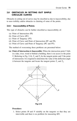
30. Circular Curves 87
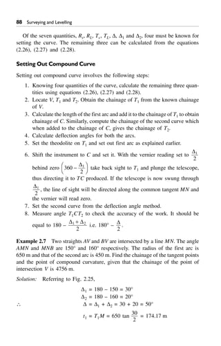
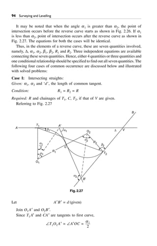
TL1 – the first tangent length (T1V)
TL2 – the second tangent length (T2V)
t1 = T1M
t2 = T2N
D = the deflection angle between the end tangents A1V and B1V
D1 = the deflection angle between the rear tangent and common tangent
D2 = the deflection angle between common tangent and the forward tangent.
Elements of the Compound Curve
From the property of circular curves.
–T1O1M = –MO1C =
D1
2
–CO2N = –NO2T2 =
D2
2
–VMC = D1 and –VNC = D2
D = D1 + D2 …(2.26)
t1 = R1 tan
D1
2
t2 = R2 tan
D2
2
Length of common tangent = MC + CN
= t1 + t2
i.e. MN = R1 tan
D1
2
+ R2 tan
D2
2
From DVMN,
VM
sin D2
= VN
sin D1
= MN
sin [ ( )]180 1 2- +D D
VM =
sin
sin ( )
D
D D
2
1 2+
MN
and VN =
sin
sin ( )
D
D D
1
1 2+
MN
Now, TL1 = t1 + VM = t1 +
sin
sin ( )
tan tan
D
D D
D D2
1 2
1
1
2
2
2 2+
+F
H
I
KR R …(2.27)
and TL2 = t2 + VN = t2 +
sin
sin ( )
tan tan
D
D D
D D1
1 2
1
1
2
2
2 2+
+F
H
I
KR R …(2.28)

31. 88 Surveying and Levelling
Of the seven quantities, Rs, RL, Ts, TL, D, D1 and D2, four must be known for
setting the curve. The remaining three can be calculated from the equations
(2.26), (2.27) and (2.28).
Setting Out Compound Curve
Setting out compound curve involves the following steps:
1. Knowing four quantities of the curve, calculate the remaining three quan-
tities using equations (2.26), (2.27) and (2.28).
2. Locate V, T1 and T2. Obtain the chainage of T1 from the known chainage
of V.
3. Calculate the length of the first arc and add it to the chainage of T1 to obtain
chainage of C. Similarly, compute the chainage of the second curve which
when added to the chainage of C, gives the chainage of T2.
4. Calculate deflection angles for both the arcs.
5. Set the theodolite on T1 and set out first arc as explained earlier.
6. Shift the instrument to C and set it. With the vernier reading set to
D1
2
behind zero 360
2
1
-F
H
I
K
D
take back sight to T1 and plunge the telescope,
thus directing it to TC produced. If the telescope is now swung through
D1
2
, the line of sight will be directed along the common tangent MN and
the vernier will read zero.
7. Set the second curve from the deflection angle method.
8. Measure angle T1CT2 to check the accuracy of the work. It should be
equal to 180 –
D D1 2
2
+
i.e. 180° –
D
2
.
Example 2.7 Two straights AV and BV are intersected by a line MN. The angle
AMN and MNB are 150° and 160° respectively. The radius of the first arc is
650 m and that of the second arc is 450 m. Find the chainage of the tangent points
and the point of compound curvature, given that the chainage of the point of
intersection V is 4756 m.
Solution: Referring to Fig. 2.25,
D1 = 180 – 150 = 30°
D2 = 180 – 160 = 20°
D = D1 + D2 = 30 + 20 = 50°
t1 = T1M = 650 tan
30
2
= 174.17 m

32. ' Surveying and Levelling
Now, TL1 = T1M + MV
= R1 tan
D1
2
+ R R1
1
2
2
2 2
tan tan
D D
+F
H
I
K
sin
sin
D
D
2
Using equations (1) and (2),
TL1 = 36 tan
D1
2
+ 36
2
48
84 5
2
1 1
tan tan
.D D
+
-F
H
I
K sin
84 5
84 5
1.
sin .
- D
38.98 = 36 tan
D1
2
+ 1.0046251 sin (84.5 – D1) 36
2
48
84 5
2
1 1
tan tan
.D D
+
-F
H
I
K
F(D1) = 36 tan
D1
2
+ 1.0046251 sin (84.5 – D1)
36
2
48
84 5
2
1 1
tan tan
.D D
+
-F
H
I
K – 38.98
Solving it by trial and a error method,
when D1 = 30°,
F(D1) = –0.0954222
when D1 = 32°,
F(D1) = –0.123610.
If D1 = 29°, F(D1) = –0.08106
If D1 = 28°, F(D1) = –0.0665
If D1 = 25°, F(D1) = –0.02419195
D1 = 23°, F(D1) = 0.008600
say D1 = 23.5° for which F(D1) = 0.000914 ª 0.
Thus, the solution is D1 = 23.5°.
D2 = 84.5 – 23.5 = 61°.
Arc length of first curve = 36 ¥ 23.5 ¥
p
180
= 14.765 chains.
Chainage of point of junction of the two curves (C)
= 30.5 + 14.765 = 45.265 chains.
Length of second curve = 48 ¥ 61 ¥
p
180
= 51.103 chains.
Chainage of last tangent point (T2)
= 45.265 + 51.103 = 96.363 chains.
For first curve:
Length of first sub-chord = 31 – 30.5 = 0.5 chains.

33. 92 Surveying and Levelling
(iii) Needs super elevation/camber on opposite edges.
(iv) At the point of reverse curvature, it is not possible to provide proper super
elevation.
Reverse curves are usually required in railways when trains are to be
changed from one line to the other line, in hilly roads and while connecting
flyovers to side lines.
Elements of a Reverse Curve
Figure 2.26 shows a general case of a reverse curve in which AV and BV are two
straights and T1CT2 is the reverse curve.
b2
a2
R2
O2
T2
P
b2
b1
a2
q
M
C
N
b1
a1
D
V
T1
R1
O1
a
1
B¢
A¢
A≤
A
B
Fig. 2.26
Let
D – the angle of deflection (–A¢VB)
R1 – the radius of first circular arc
R2 – the radius of second circular arc.
T1, T2 – the tangent points
C – the point of reverse curvature
a1 – the angle subtended at the centre by the first curve
a2 – the angle subtended at the centre by the second curve
b1 – the angle of deflection between the first tangent and the common tangent
b2 – the angle of defleciton between the second tangent and the common
tangent.
Join T1T2. Drop perpendiculars O1M and O2N to line T1T2. Through O1P draw
O1P parallel to T1T2 cutting O2N produced at P.

34. Circular Curves '!
Let A¢, B¢ be the points where common tangent intersects the first and the
second tangents respectively.
The points O1, C and O2 are in a line, since C is the point on both curves and
A¢B¢ is common tangent.
Since A¢T1 and A¢C are tangents to first curve,
–A≤A¢E = –T1O1C = a1
Similarly, –A¢B¢V = –T2O2C = a2
From DA¢VB¢, a1 = D + a2
or D = a1 – a2 …(2.29)
Similarly, from D T1 T2V,
b1 = D + b2
or D = b1 – b2 …(2.30)
From equations (1) and (2), we get
a1 – a2 = b1 – b2
or a1 – b1 = a2 – b2 …(a)
Now, –T1O1M + –O1T1M = 90° = –O1T1M + –A¢T1M
–T1O1M = –A¢T1M = b1 …(b)
Similarly, –T2O2N = b2 …(c)
T1M = R1sin b1
T2N = R2 sin b2
MN = O1P = (R1 + R2) sin (a2 – b2)
Tangent length
T1T2 = T1 M + MN + T2N
= R1 sin R1 + (R1 + R2) sin (a2 – b2) + R2 sin b2
O2P = O2N + NP = O2N + O1M
= R2 cos b2 + R1 cos b1 …(d)
and also O2P = (R1 + R2) cos (a2 – b2) …(e)
From equations (d) and (e), we get
(R1 + R2) cos (a2 – b2) = R1 cos b1 + R2 cos b2
cos (a2 – b2) =
R R
R R
1 1 2 2
1 2
cos cosb b+
+
…(2.31a)
Since a2 – b2 = a1 – b1,
cos (a1 – b1) =
R R
R R
1 1 2 2
1 2
cos cosb b+
+
…(2.31b)

35. ' Surveying and Levelling
It may be noted that when the angle a1 is greater than a2, the point of
intersection occurs before the reverse curve starts as shown in Fig. 2.26. If a1
is less than a2, point of intersection occurs after the reverse curve as shown in
Fig. 2.27. The equations for both the cases will be identical.
Thus, in the elements of a reverse curve, these are seven quantities involved,
namely, D, a1, a2, b1, b2, R1 and R2. Three independent equations are available
connecting these seven quantities. Hence, either 4 quantities or three quantities and
one conditional relationship should be specified to find out all seven quantities. The
following four cases of common occurrence are discussed below and illustrated
with solved problems:
Case I: Intersecting straights:
Given: a1, a2 and ‘d’, the length of common tangent.
Condition: R1 = R2 = R
Required: R and chainages of T1, C, T2, if that of V are given.
Referring to Fig. 2.27
C
a1
b2
T2
O2
A¢
D V
B
a1
2
T1
A
B¢
a2
O1
R1a1
b1
R2
a2
Fig. 2.27
Let A¢B¢ = d (given)
Join O1A¢ and O2B¢.
Since T1 A¢ and CA¢ are tangents to first curve,
–T1O1A¢ = –A¢OC =
a1
2

36. '$ Surveying and Levelling
A¢T1 = R tan
a1
2
= 1410.32 tan
17 5
2
.
= 217.07 m
Chainage of first tangent point (T1)
= 895 – 217.07 = 677.93 m
Arc length of first curve = R
a1
2
¥
p
180
= 1410.32 ¥ 17.5 ¥
p
180
= 430.76 m
Chainage of point of reverse curve, C,
= 677.93 + 430.76 = 1108.69 m Ans.
Length of arc of second curve
= 1410.32 ¥ 27.333 ¥
p
180
= 672.80 m
Chainage of second tangent point (T2)
= 1108.69 + 672.80
= 1781.49 m Ans.
Case II: Intersecting straights
Given: Length of the line joining tangent points T1 and T2, angles b1 and b2.
Condition: R1 = R2 = R
Required: Common radius R.
Referring to Fig. 2.26,
Let T1T2 = L
O1M = R cos P1 = PN
O2 N = R cos b2
Let –O2O1P = q. Then from DO2O1P,
sin q =
O P
O O
2
1 2
=
R R
R R
cos cosb b1 2+
+
=
cos cosb b1 2
2
+
…(2.34)
Hence, q may be found.
Then, L = T1M + MN + NT2
= R sin b1 + (R + R) cos q + R sin b2

37. Circular Curves '%
R = L
sin cos sinb q b1 22+ +
…(2.35)
Hence, R can be found.
Example 2.10 Two straights AT1 and BT2 meet at vertex V. A reverse curve of
common radius R having T1 and T2 as tangent points is to be introduced. The
angles VT1T2 and VT2T1 measured at T1 and T2 are 45°30¢ and 25°30¢, respec-
tively. The distance T1T2 is equal to 800 m. Determine the common radius and the
central angles for the two arcs.
Solution: Referring to Fig. 2.26,
L = 800 m
b1 = 45°30¢ = 45.5° b2 = 25°30¢ = 25.5°
D = b1 – b2 = 45.5° – 25.5° = 20°
sin q =
cos cosb b1 2
2
+
=
cos . cos .45 5 25 5
2
+
= 0.8017
q = 53.2972°
R = L
sin cos sinb q b1 22+ +
= 800
45 5 2 53 2972 25 5sin . cos . sin .+ +
= 342.14 m Ans.
a1 = b1 + (90 – q) = 45.5 + 90 – 53.2972 = 82.2028°
= 82°12 ¢10≤ Ans.
a2 = b1 – D = 82°12¢10≤ – 20°0¢0≤
= 62°12¢10≤ Ans.
Case III: Intersecting straights.
Given: T1 T2 = L, b1, b2 and R1 or R2.
Required: To find the other radius.
Referring to Fig. 2.26,
MN = O1P = O O O P1 2
2
2 2+
O1O2 = R1 + R2
O2P = O2N + NP
= O2N + O1M
= R2 cos b2 + R1 cos b1

38. Circular Curves ''
7.7448 R2 = 47.9388
R2 = 6.190 chains Ans.
[Note: R2
2
term gets cancelled because right hand side term is R2
2
sin2
b2 and left-
hand side term is R2
2
– R2
2
cos2
b2 which is also R2 sin2
b2]
Now, sin q =
O P
O O
2
1 2
=
R R
R R
1 1 2 2
1 2
cos cosb b+
+
=
8 32 14 619 16 48
8 619
cos . cos
.
∞ ¢ + ∞ ¢
+
= 0.8945
q = 63.443° = 63°27¢
a1 = b1 + 90 – q = 32°14¢ + 90 – 63°27¢
= 58°47¢ = 58.783°
a2 = 90 – q + b2 = 90 – 63°27¢ + 16°48¢
= 43°21¢ = 43.35°
The length of the first curve
= R1 ¥ a1 ¥
p
180
= 8 ¥ 58.783 ¥
p
180
= 8.208 chains. Ans.
The length of the second curve
= R2 ¥ a2 ¥
p
180
= 6.19 ¥ 43.35 ¥
p
180
= 4.683 chains. Ans.
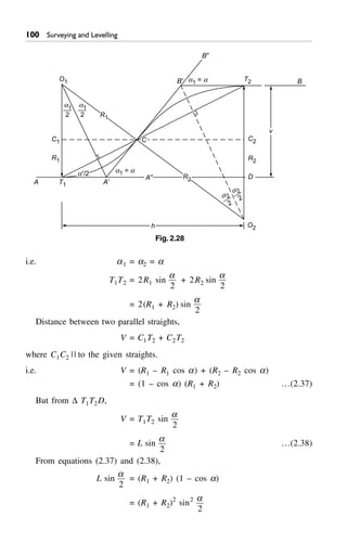
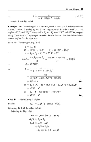
Case IV: Parallel straights
Given: R1, R2 and the central angles.
Required: Elements of reverse curve. Referring to Fig. 2.28
Let C be the point of reverse curve.
a1 – central angle T1O1C
a2 – central angle T2O2C
From the property of circular curve, the angle between first tangent and
common tangent,
–A≤A¢C = –T1OC = a1 and
–B≤B¢ T1 = –T2OC = a2
since BB¢ || AA¢,
–A≤A¢ C = –B≤B¢ T1

39. Surveying and Levelling
i.e. a1 = a2 = a
T1T2 = 2R1 sin
a
2
+ 2R2 sin
a
2
= 2(R1 + R2) sin
a
2
Distance between two parallel straights,
V = C1T2 + C2T2
where C1C2 || to the given straights.
i.e. V = (R1 – R1 cos a) + (R2 – R2 cos a)
= (1 – cos a) (R1 + R2) …(2.37)
But from D T1T2D,
V = T1T2 sin
a
2
= L sin
a
2
…(2.38)
From equations (2.37) and (2.38),
L sin
a
2
= (R1 + R2) (1 – cos a)
= (R1 + R2)2
sin2 a
2
T1
R1
C1
R2
a1 = a
A¢
O1
C2
BT2B¢ a1 = a
B≤
a1
2
a1
2
a 2
2
a 2
2
A
v
a¢/2
R1
R2 D
C
A≤
h O2
Fig. 2.28

40. Surveying and Levelling
= 150 ¥ 27.266 ¥
p
180
= 71.38 m Ans.
Chainage of T1 = 1988 m
Chainage of point of reverse curve
= 1988 + 57.11 = 2045.11 m Ans.
Chainage of second tangent point T2
= 2045.11 + 71.38 = 2116.49 m Ans.
Example 2.13 A reverse curve is to be set out between two parallel tangents
10 m apart. The distance between the tangent points measured parallel to the
tangents is 80 m. If the radius of the first branch is 150 m, calculate the radius
of the second branch. Also calculate the lengths of the two branches. What would
be the equal radius of the branches of the two reverse curve?
Solution: Referring to Fig. 2.28,
v = 10 m h = 80 m R1 = 150 m
tan
a
2
=
v
h
=
10
80
a = 14.25°
h = R1 sin a + R2 sin a
Substituting the values of h, R1 and a, we get
80 = 150 sin 14.25 + R2 sin 14.25
R2 sin 14.25 = 43.077
R2 = 175 m Ans.
Length of first curve
= R1 ¥ a ¥
p
180
= 150 ¥ 14.25 ¥
p
180
= 37.31 m Ans.
Length of second curve
= R2 ¥ a ¥
p
180
= 175 ¥ 14.25 ¥
p
180
= 43.52 m Ans.