Downloaded 106 times


![DISTANCE MEASUREMENT 25
out to correct level as well as to correct line. Levels are carried down from a known datum, may
be at the side of the excavated shaft at top, using a very long tape hanging vertically and free of
restrictions to carry out operation in a single stage. In the case when a very long tape is not
available, the operation is carried out by marking the separate tape lengths in descending order.
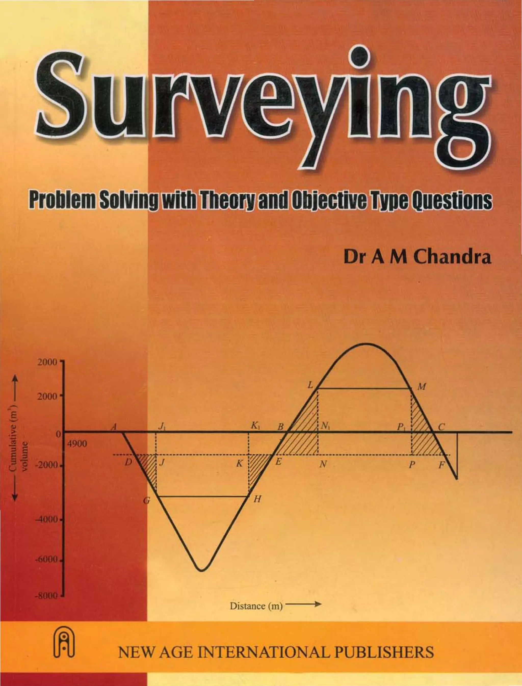
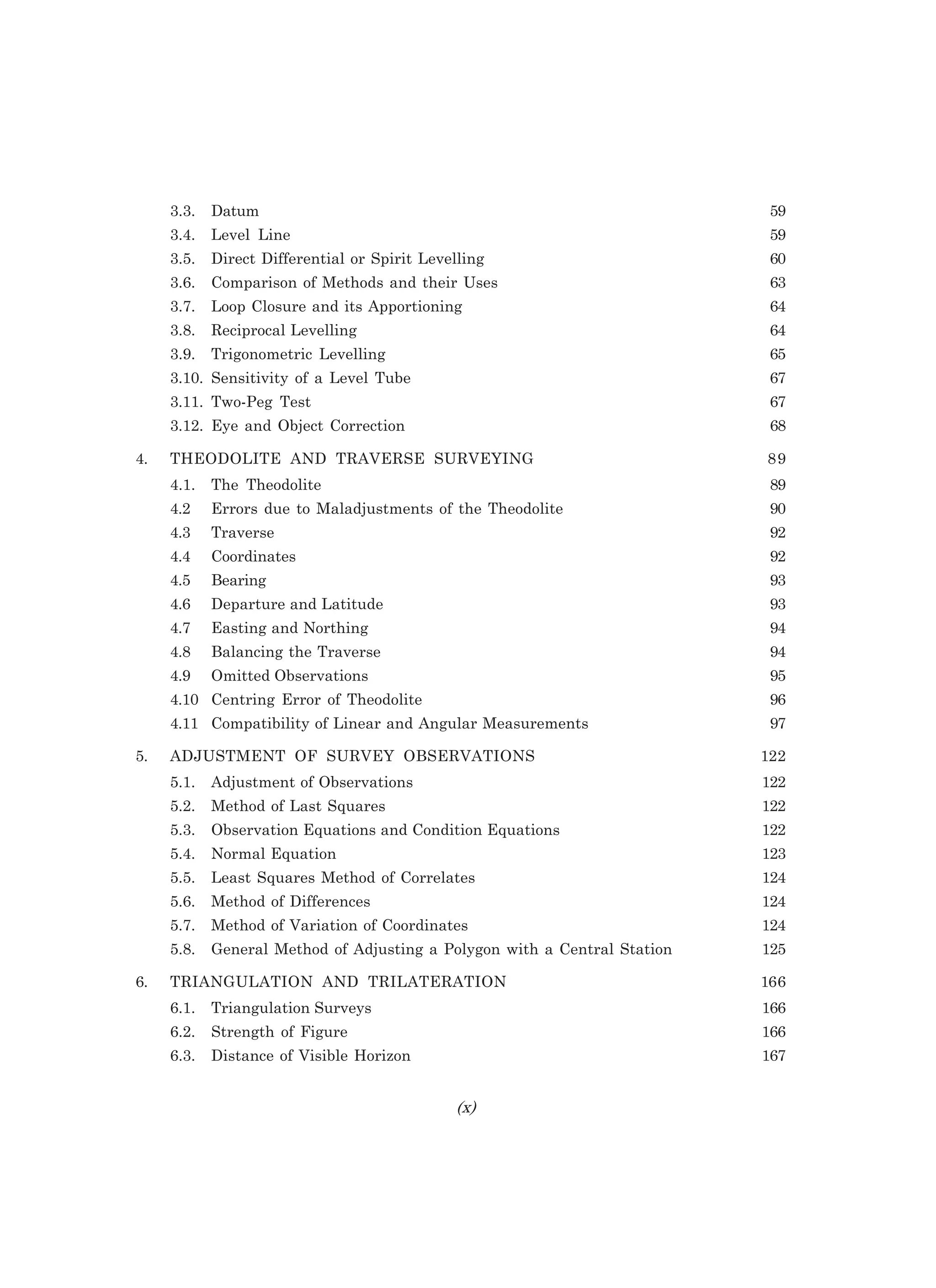
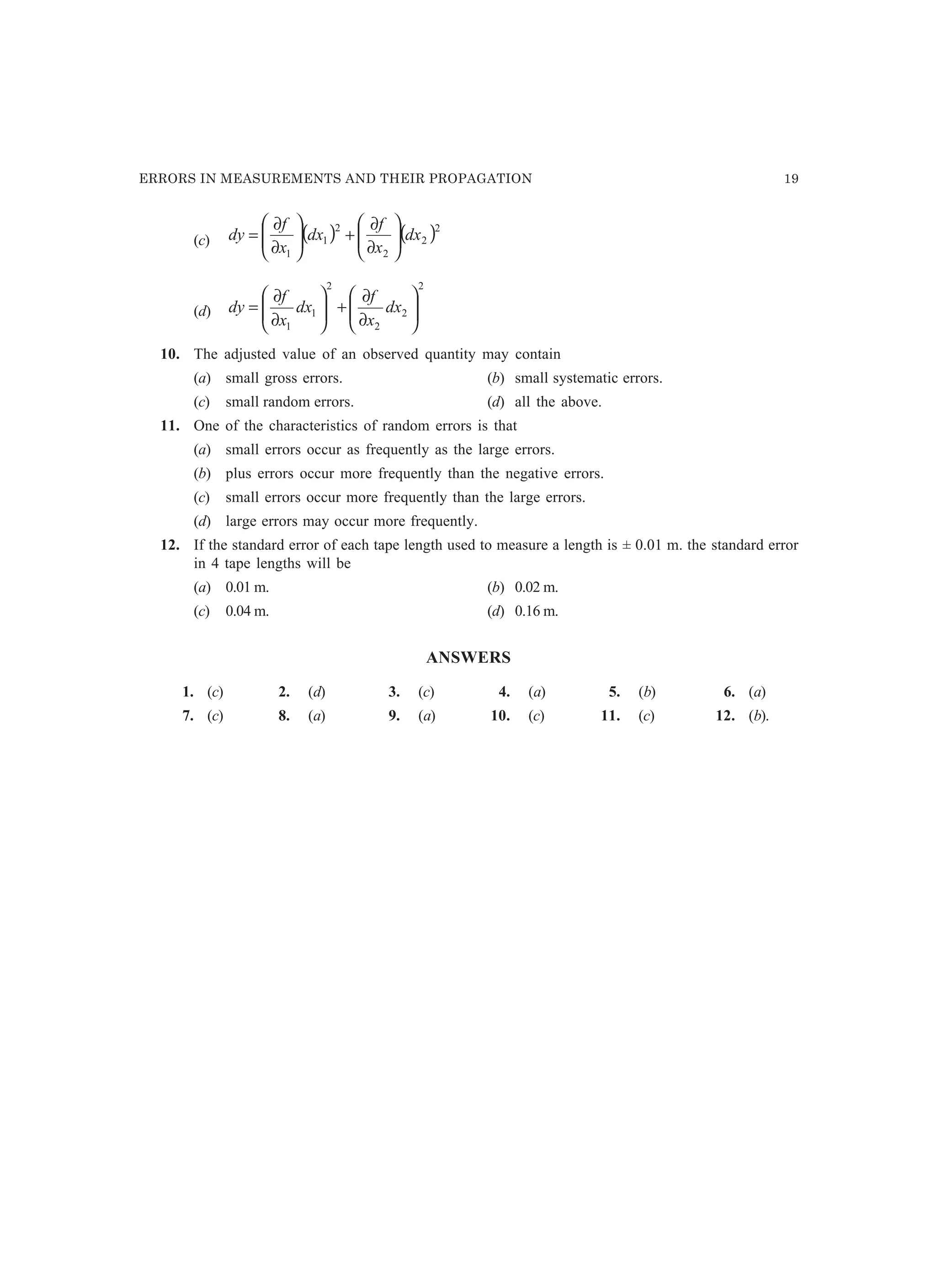
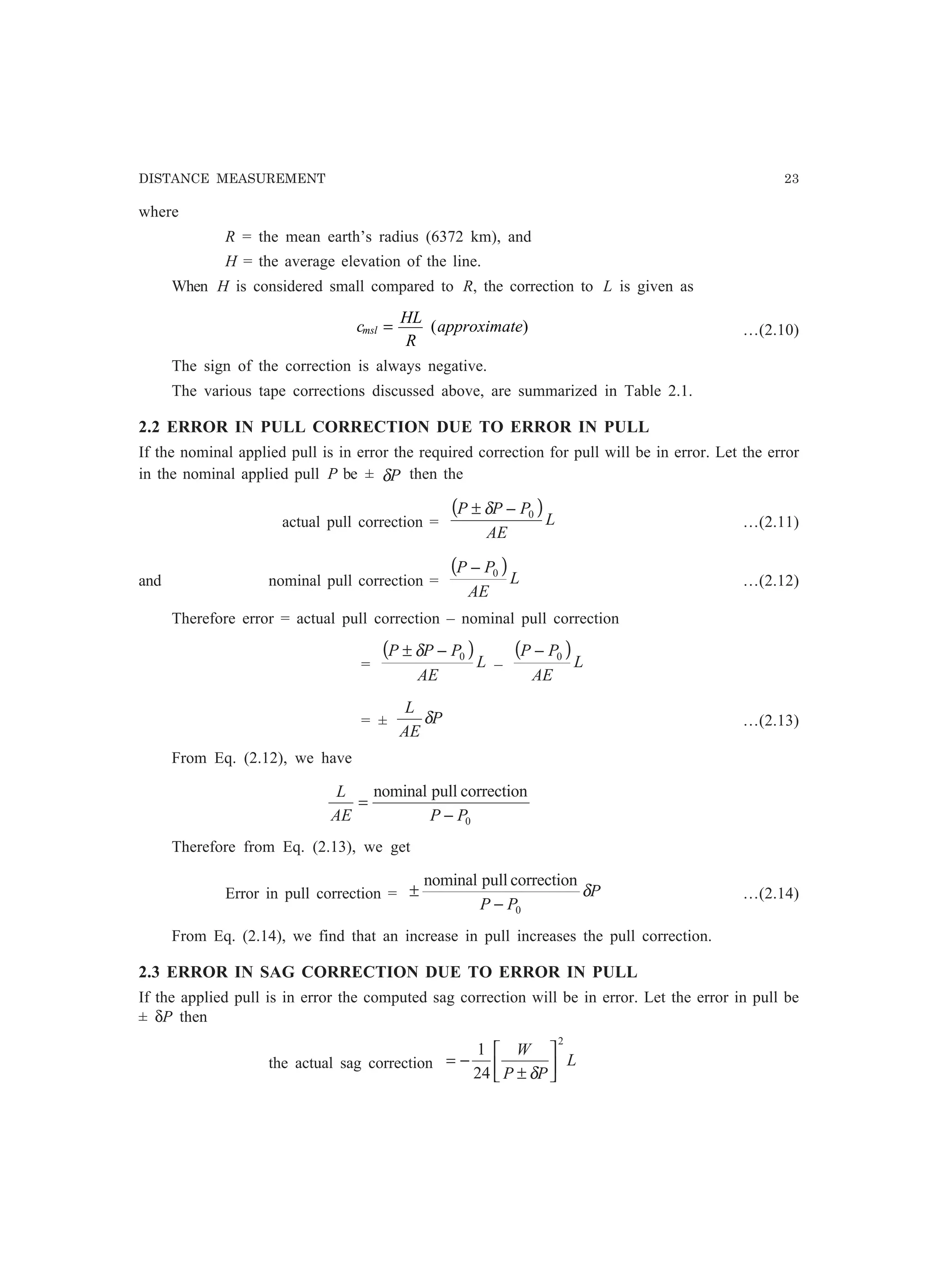
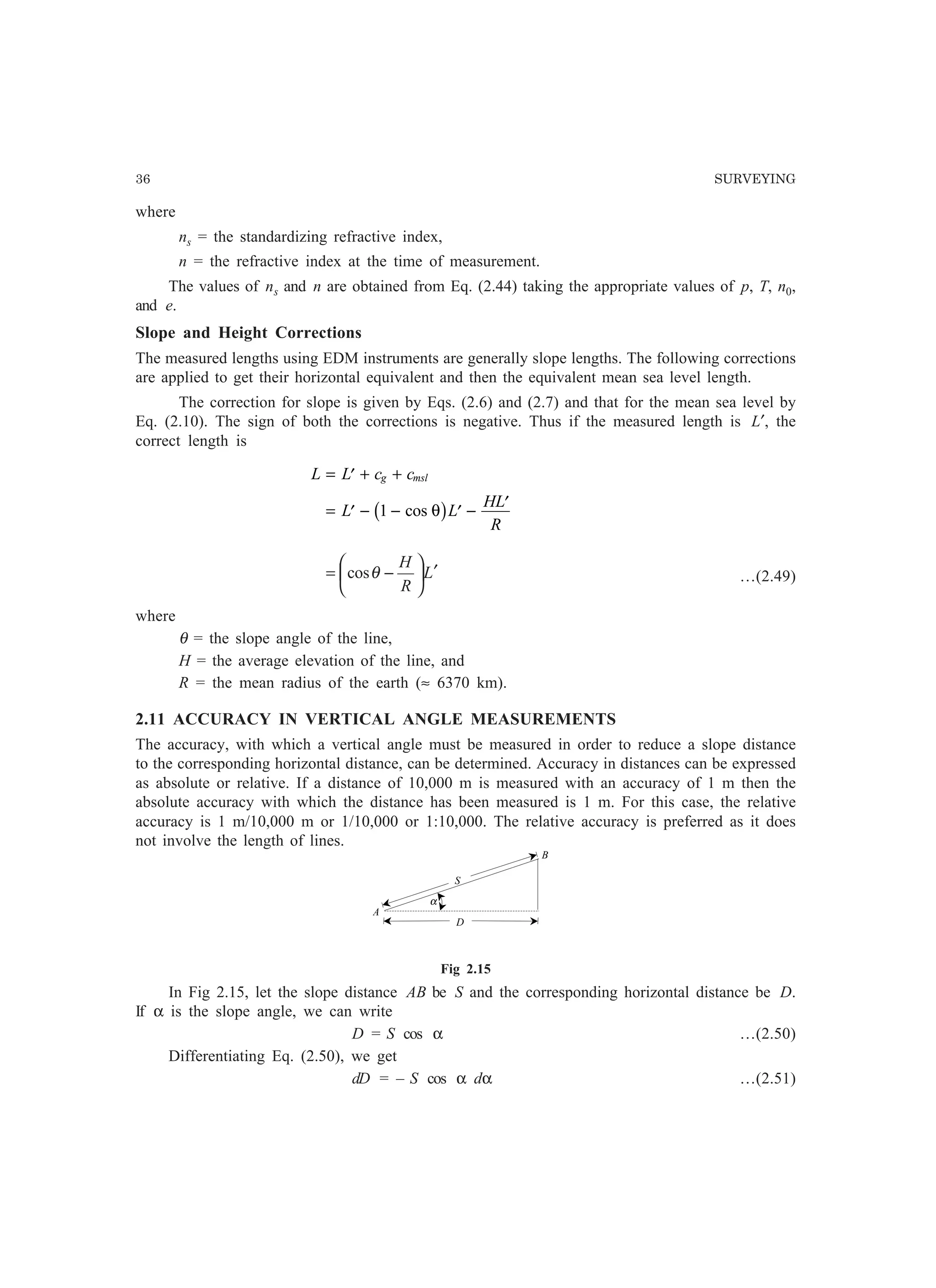
The elongation in the length of the tape AC hanging vertically from a fixed point A due to
its own weight as shown in Fig. 2.5, can be determined as below.
Let s = the elongation of the tape,
g = the acceleration due to gravity,
x = the length of the suspended tape used
for the measurement,
(l – x) = the additional length of the tape not required
in the measurements,
A = the area of cross-section of the tape,
E = the modulus of elasticity of the tape material,
m = the mass of the tape per unit length,
M = the attached mass,
l = the total length of the tape, and
P0 = the standard pull.
The tension sustained by the vertical tape due to self-loading is maximum at A. The tension
varies with y considered from free-end of the tape, i.e., it is maximum when y is maximum and,
therefore, the elongations induced in the small element of length dy, are greater in magnitude in the
upper regions of the tape than in the lower regions.
Considering an element dy at y,
loading on the element dy = mgy
and extension over the length dy
AE
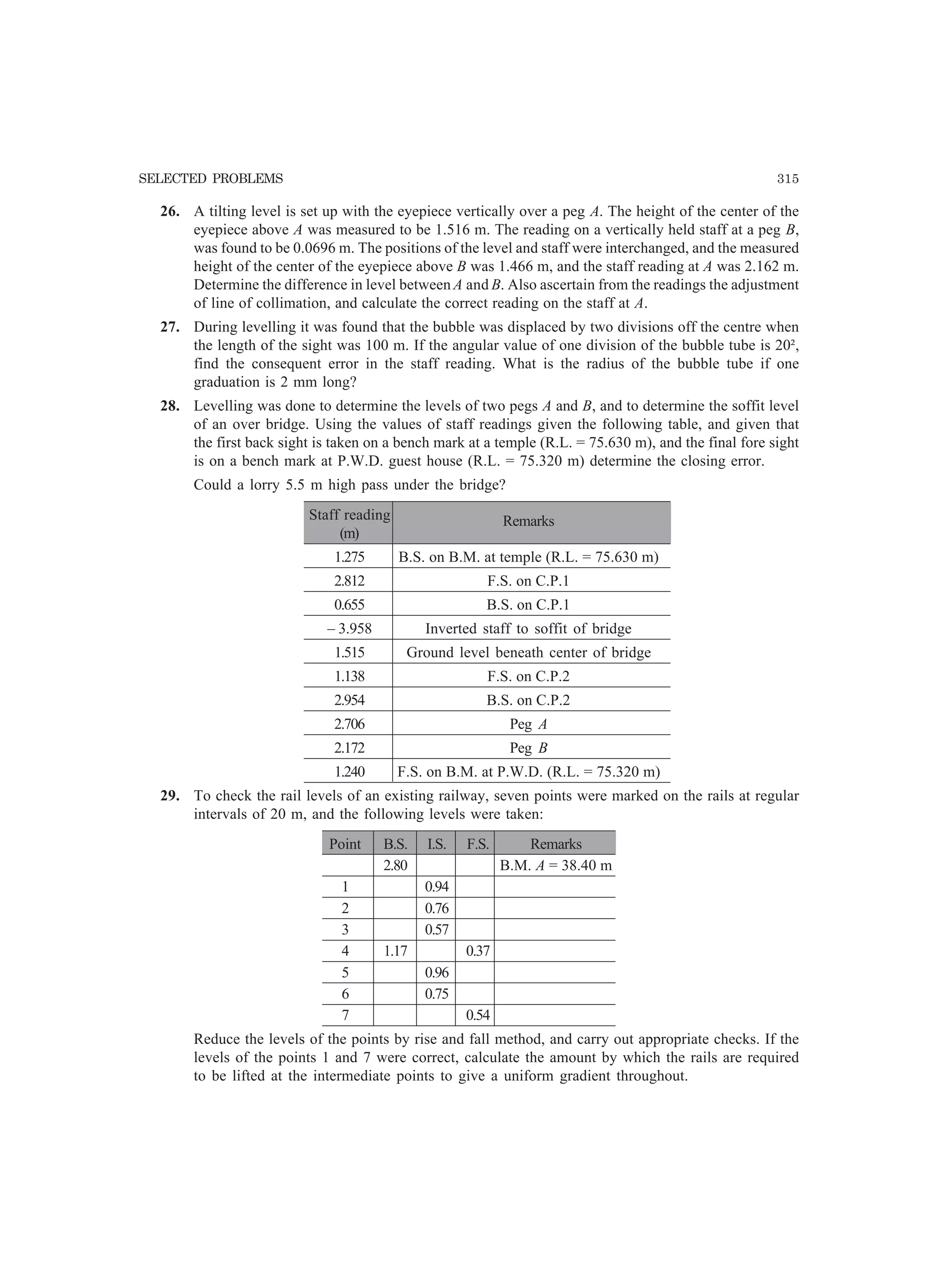
dy
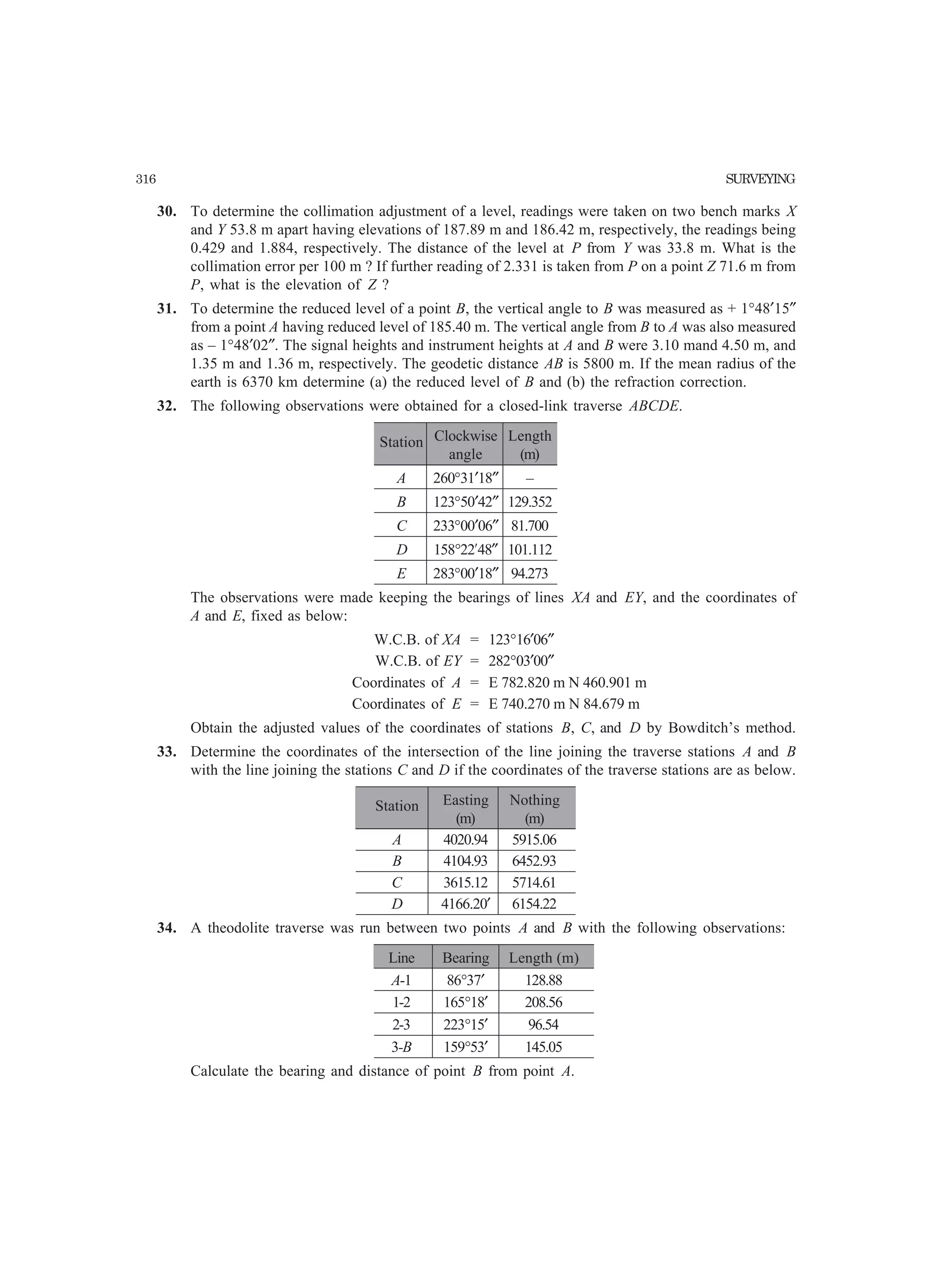
mgy=
Therefore, extension over length AB, Ex ( )∫ −
=
l
xl AE
dy
mgy
( )
constant
2
2
+
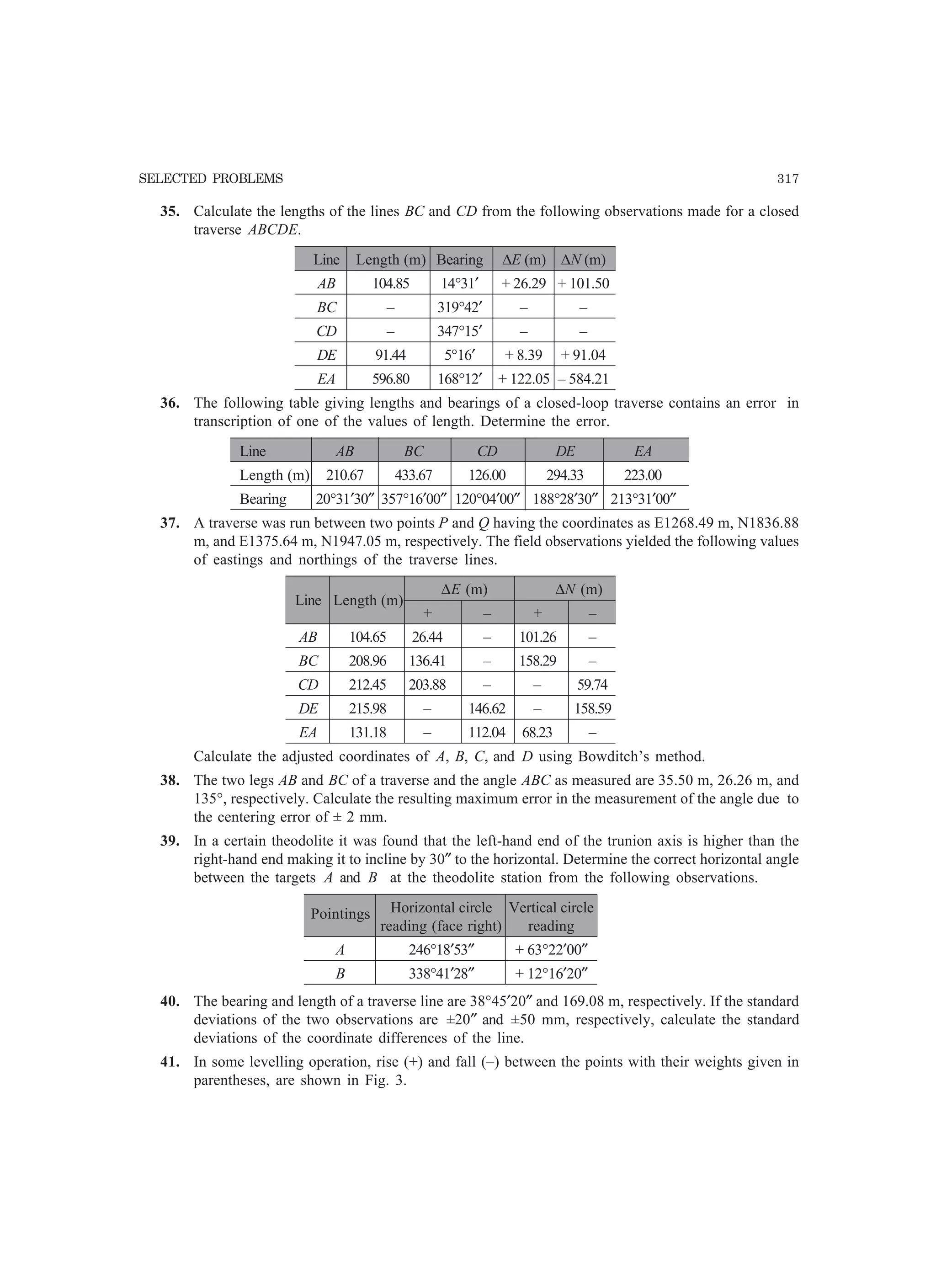
=
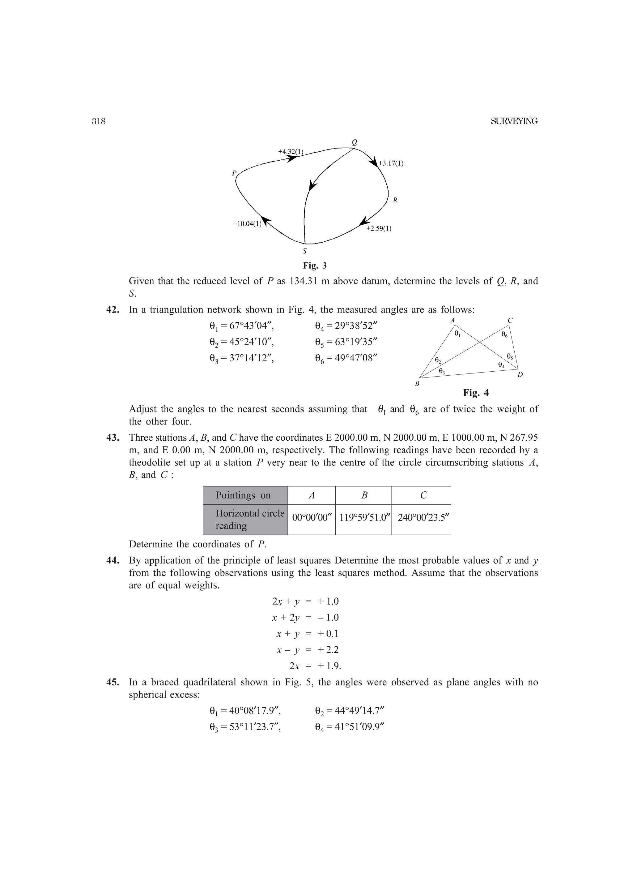
−
l
xl
y
AE
mg
We have Ex = 0 when y = 0, therefore the constant = 0. Thus
( )[ ]22
2
xll
AE
mg
Ex −−=
−
=
2
2 xl
AE
mgx
…(2.16)
To ensure verticality of the tape and to minimize the oscillation, a mass M may be attached
to the lower end A. It will have a uniform effect over the tape in the elongation of the tape.
x
l
dy
y
(l−x)
A
B
Support
Fixed end of tape
Measured length
Free end of tape
C
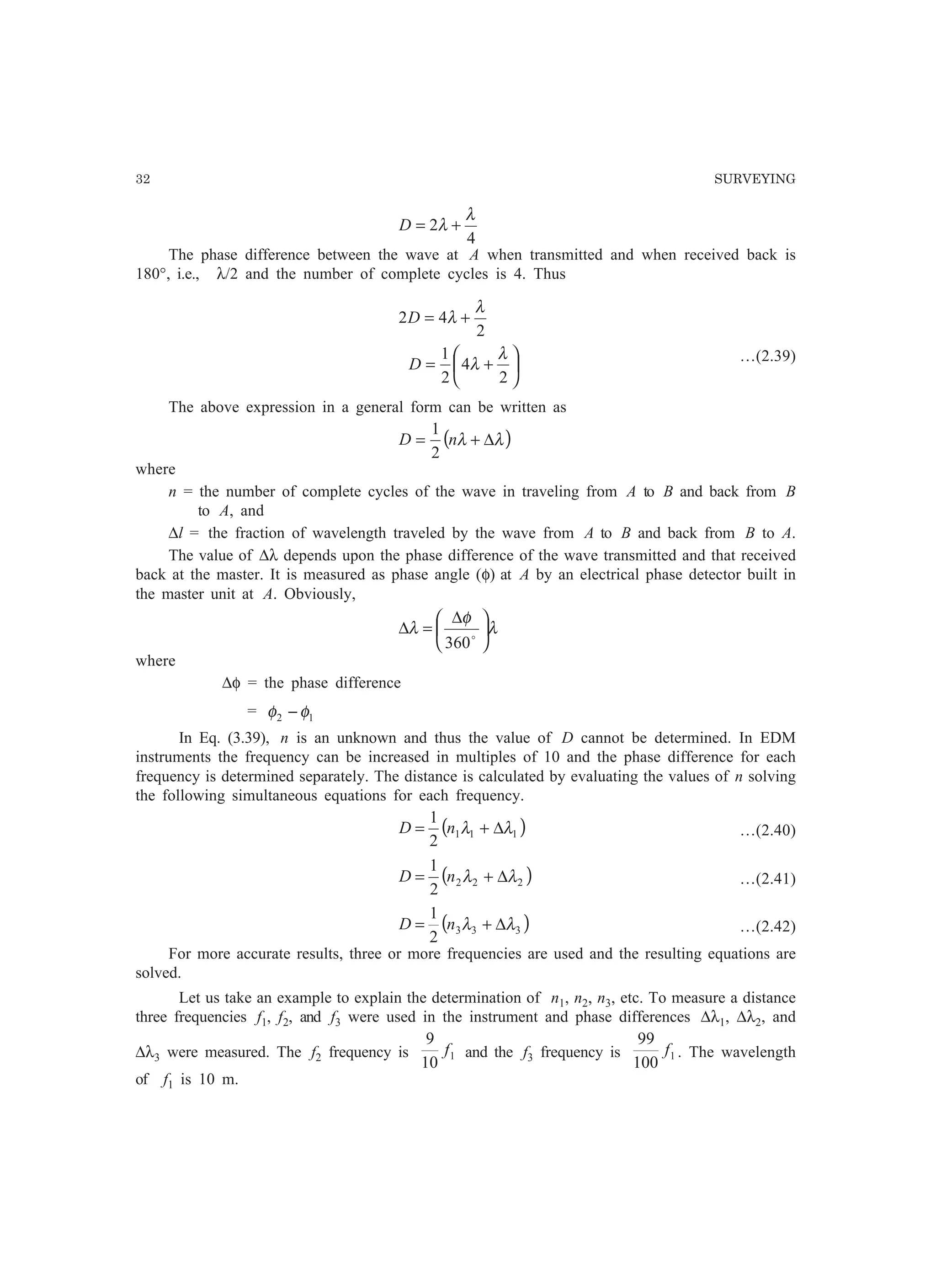
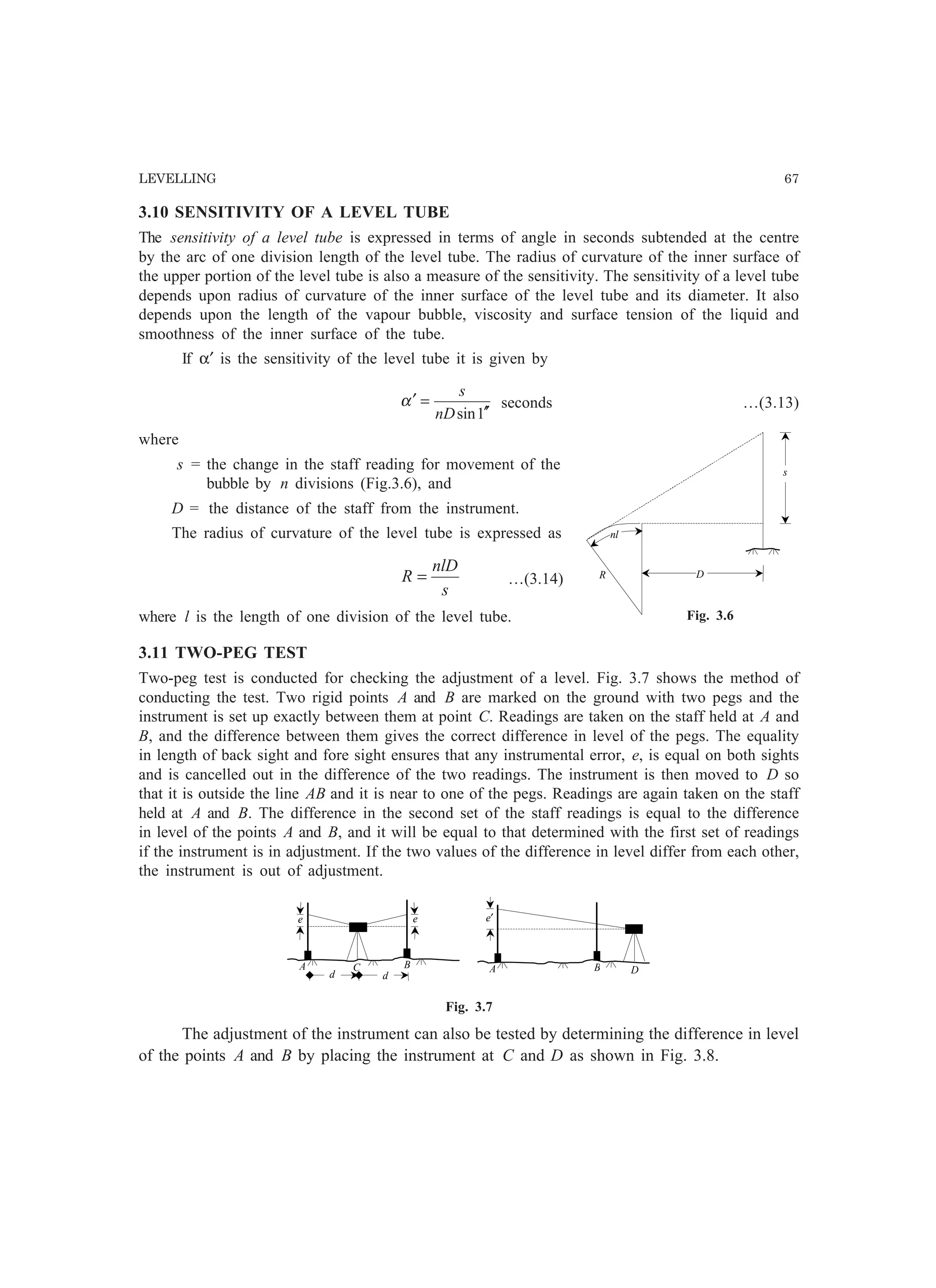
Fig. 2.5](https://image.slidesharecdn.com/surveyingproblemsolving-150308103254-conversion-gate01/75/Surveying-problem-solving-38-2048.jpg)
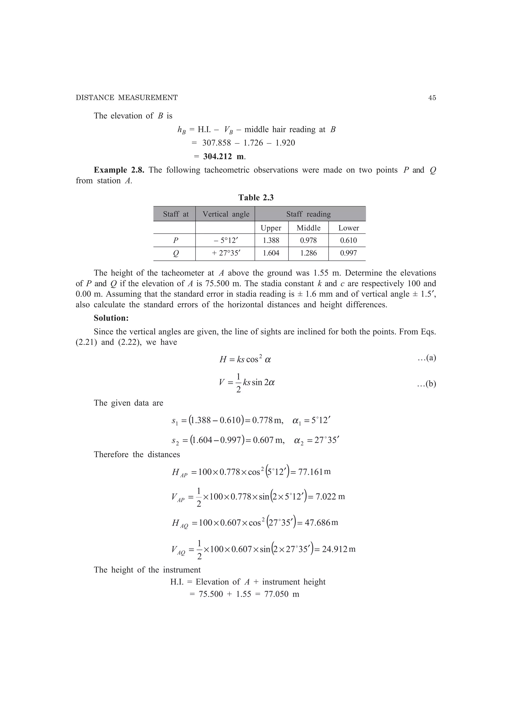
![38 SURVEYING
D AB=
= ° ′ ′′
cos
. × cos ( )
α
347 41 2 17 26 = 347.13 m.
Alternatively, for small angles,
25
1
=α radians = 13712 ′′′o , which gives the same value of
D as above.
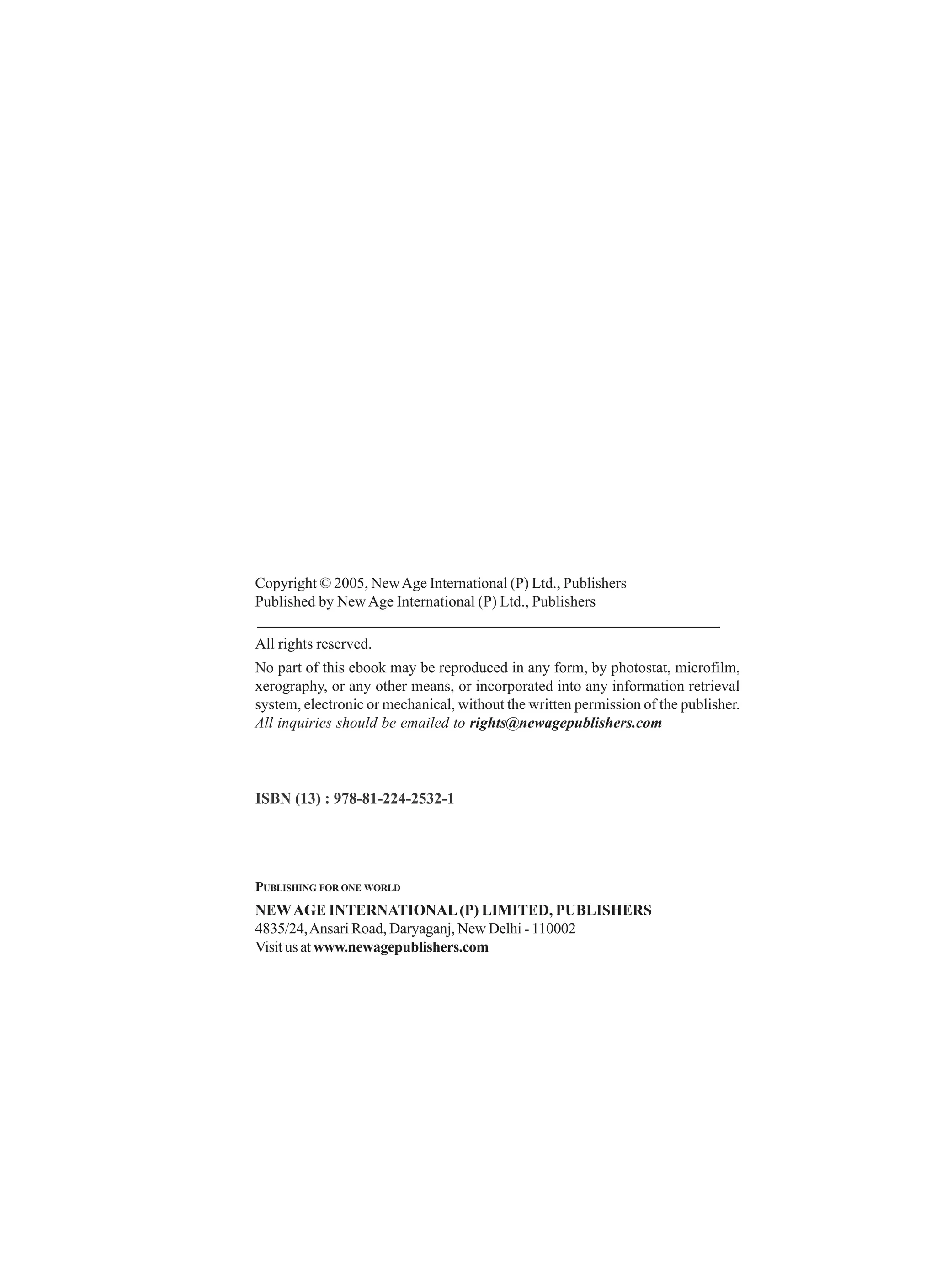
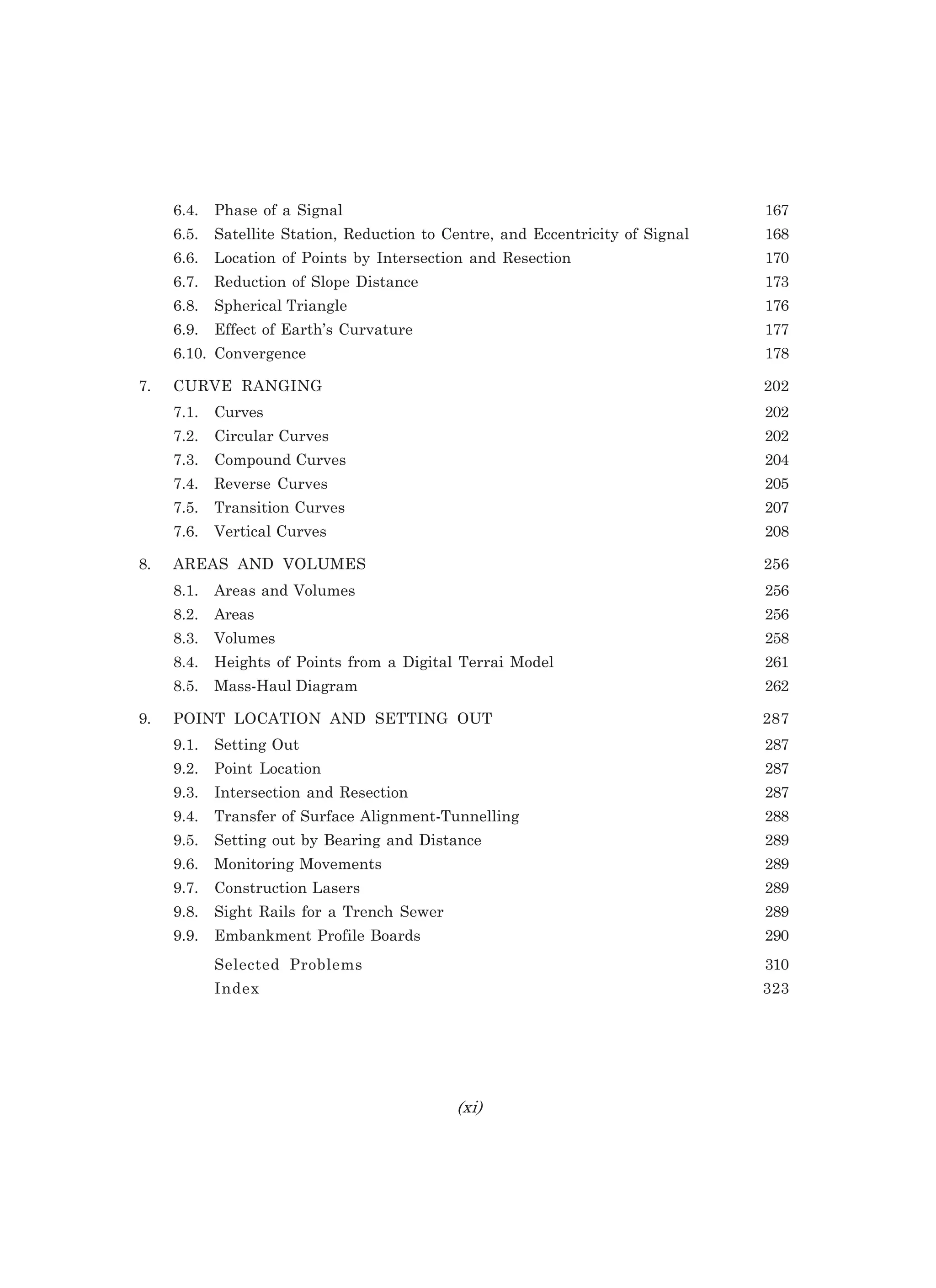
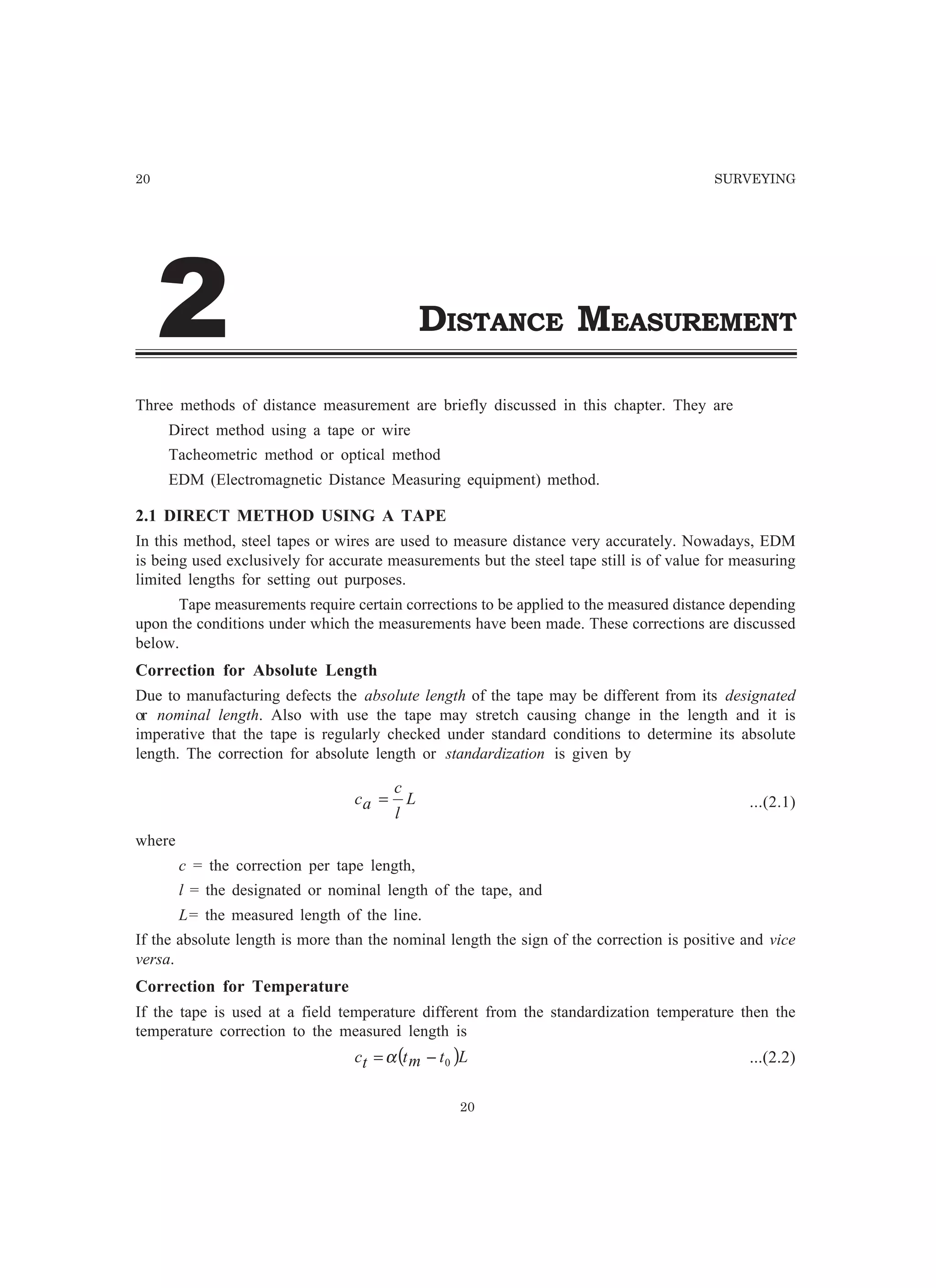
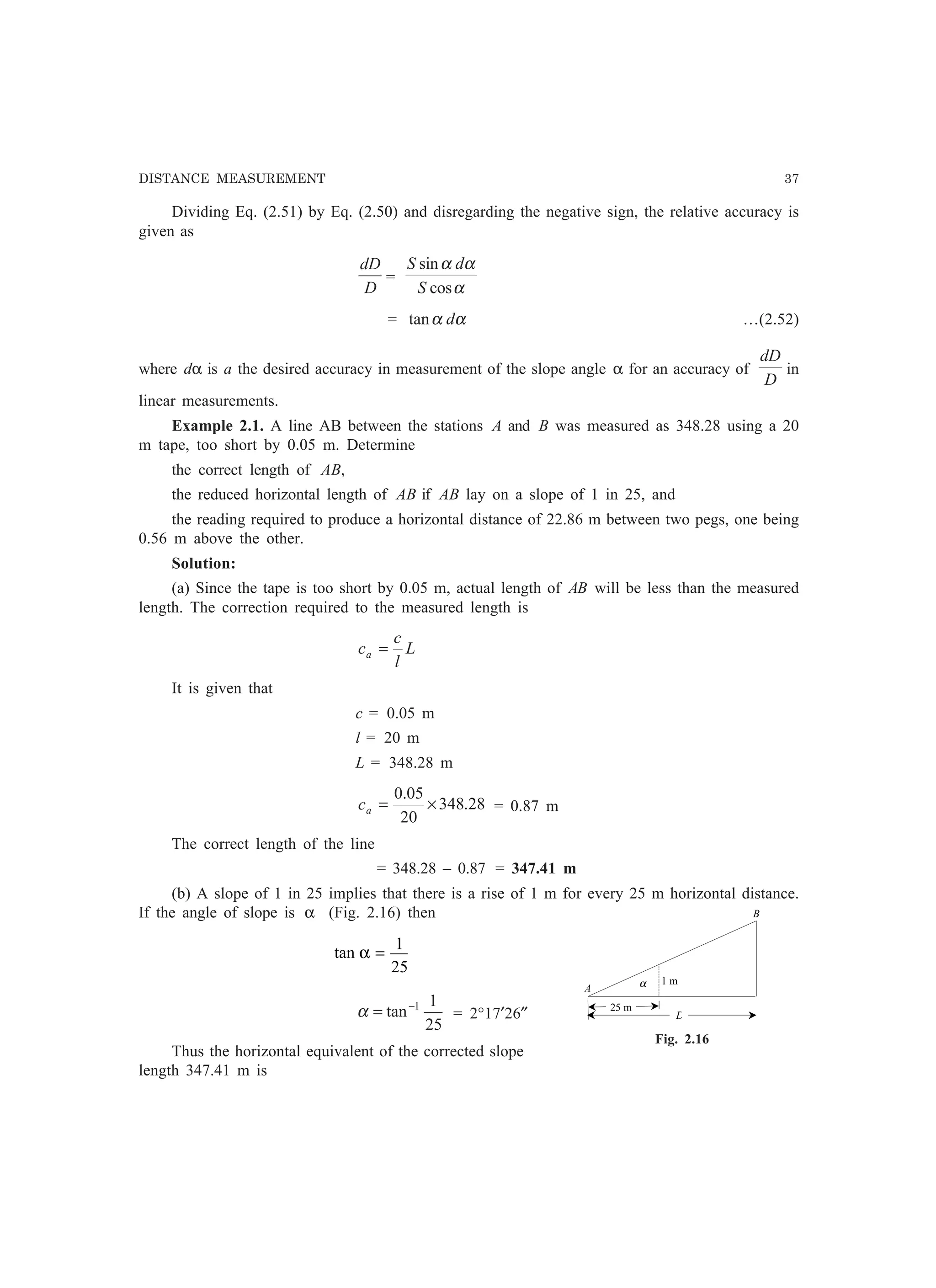
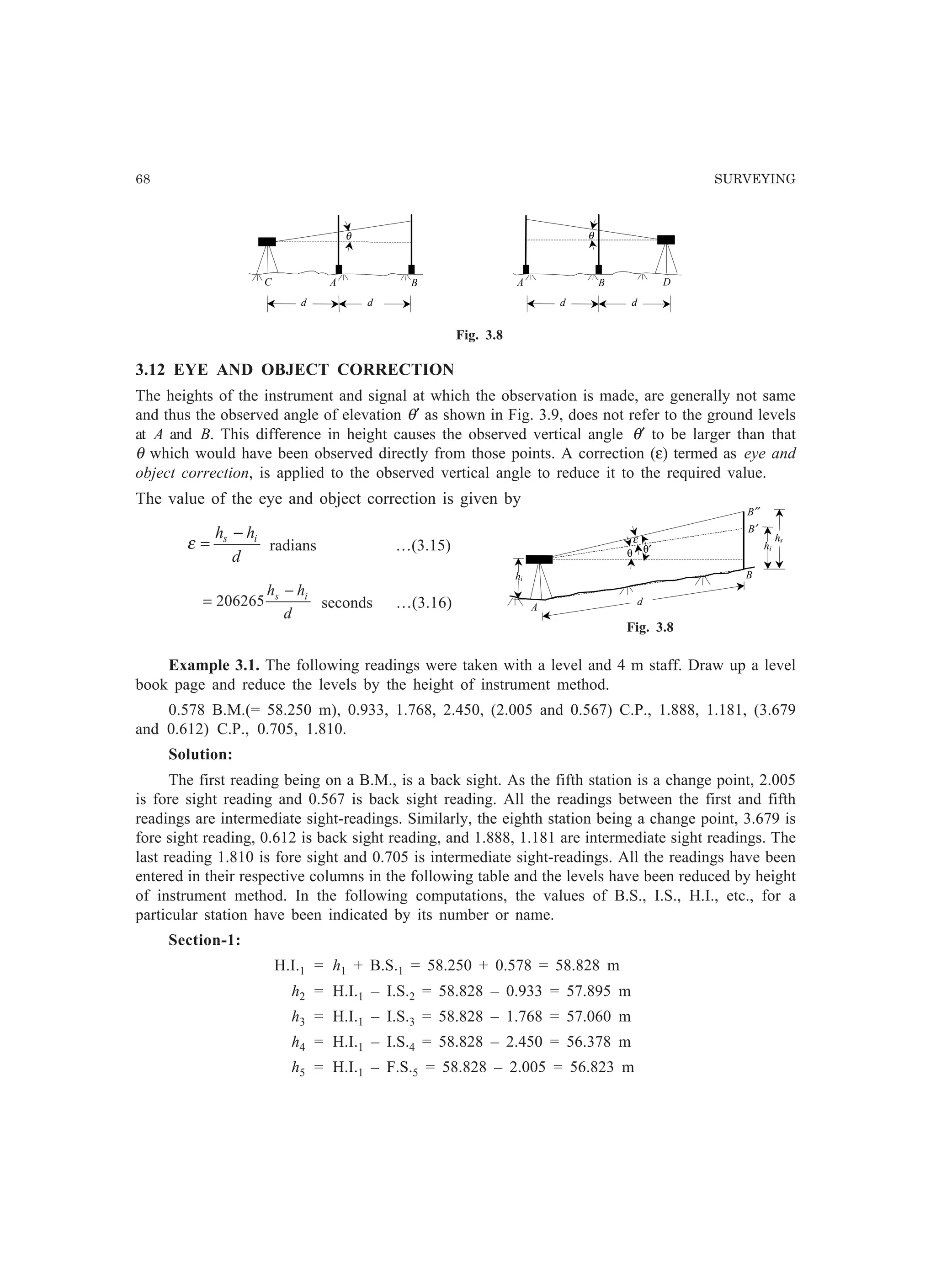
From Fig. 2.17, we have
22
22
56.086.22 +=
+= CBACAB
= 22.87 m
Therefore the reading required
= 22.87 + 87.22
0.20
05.0
× = 22.93 m
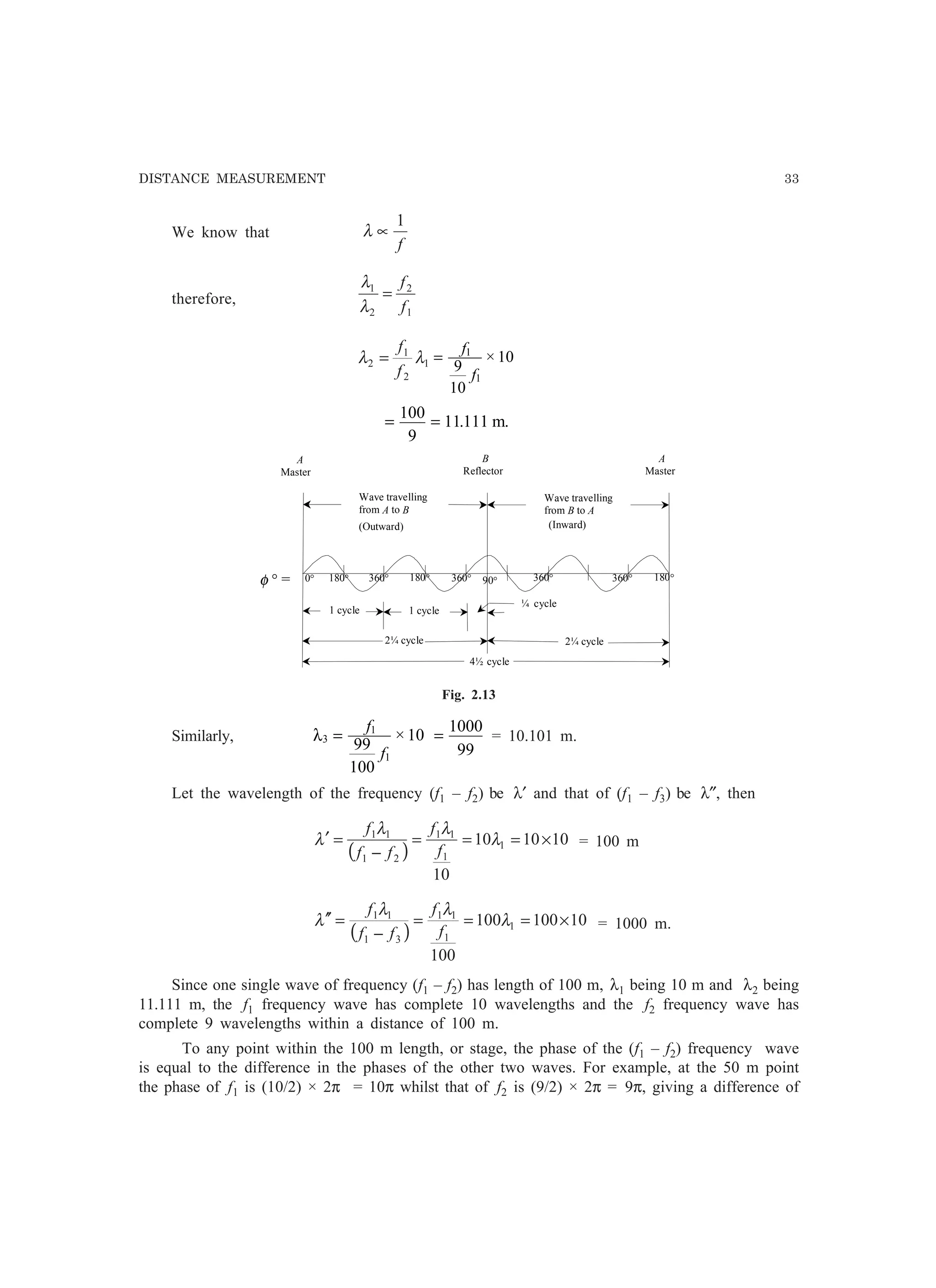
Example 2.2. A tape of standard length 20 m at 85°F was used to measure a base line. The
measured distance was 882.50 m. The following being the slopes for the various segments of the
line:
Segment length (m) Slope
100 2°20′
150 4°12′
50 1°06′
200 7°48′
300 3°00′
82.5 5°10′
Calculate the true length of the line if the mean temperature during measurement was 63°F and
the coefficient of thermal expansion of the tape material is 6.5 × 10⁻⁶
per °F.
Solution:
Correction for temperature
( )Lttc mt 0−=α
( ) 50.8828563105.6 6
×−××= −
= – 0.126 m
Correction for slope
( )[ ]Lcs αcos1−Σ=
( ) ( ) ( )
( ) ( ) ( ) 5.82015cos1300003cos1200847cos1
50601cos1150214cos1100022cos1
×′−+×′−+×′−
+×′−+×′−+×′−=
ooo
ooo
= –3.092 m
0.56 mA
B
C22.86 m
Fig. 2.17](https://image.slidesharecdn.com/surveyingproblemsolving-150308103254-conversion-gate01/75/Surveying-problem-solving-51-2048.jpg)

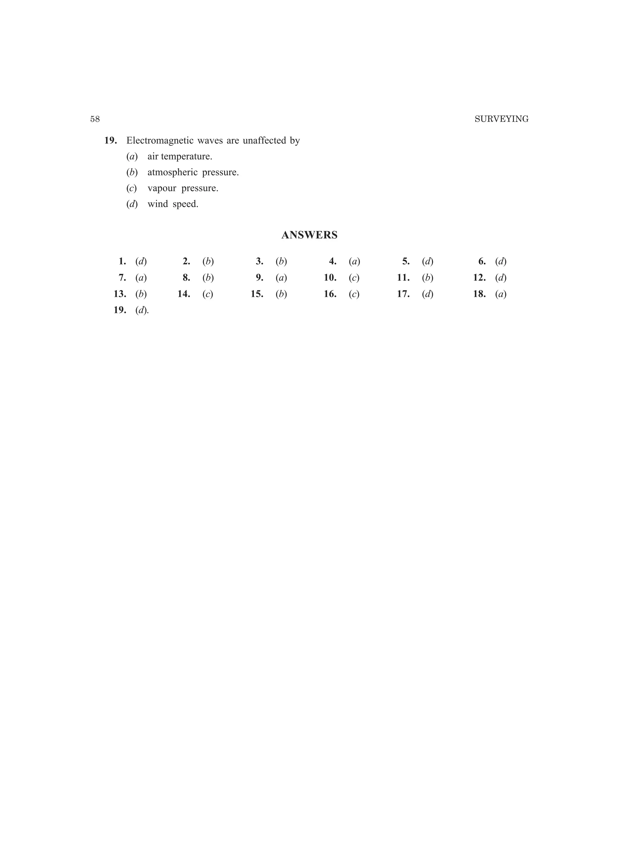
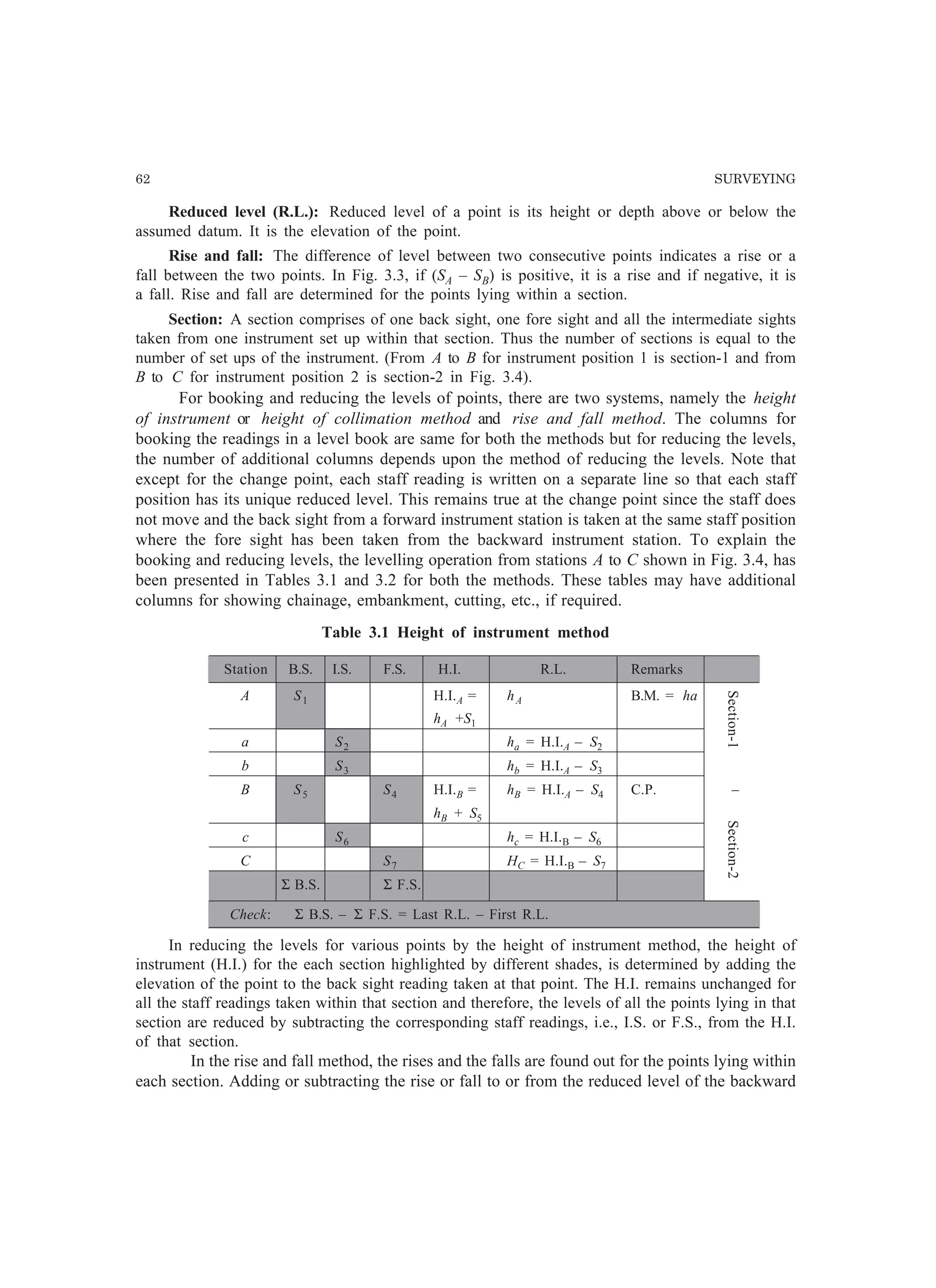
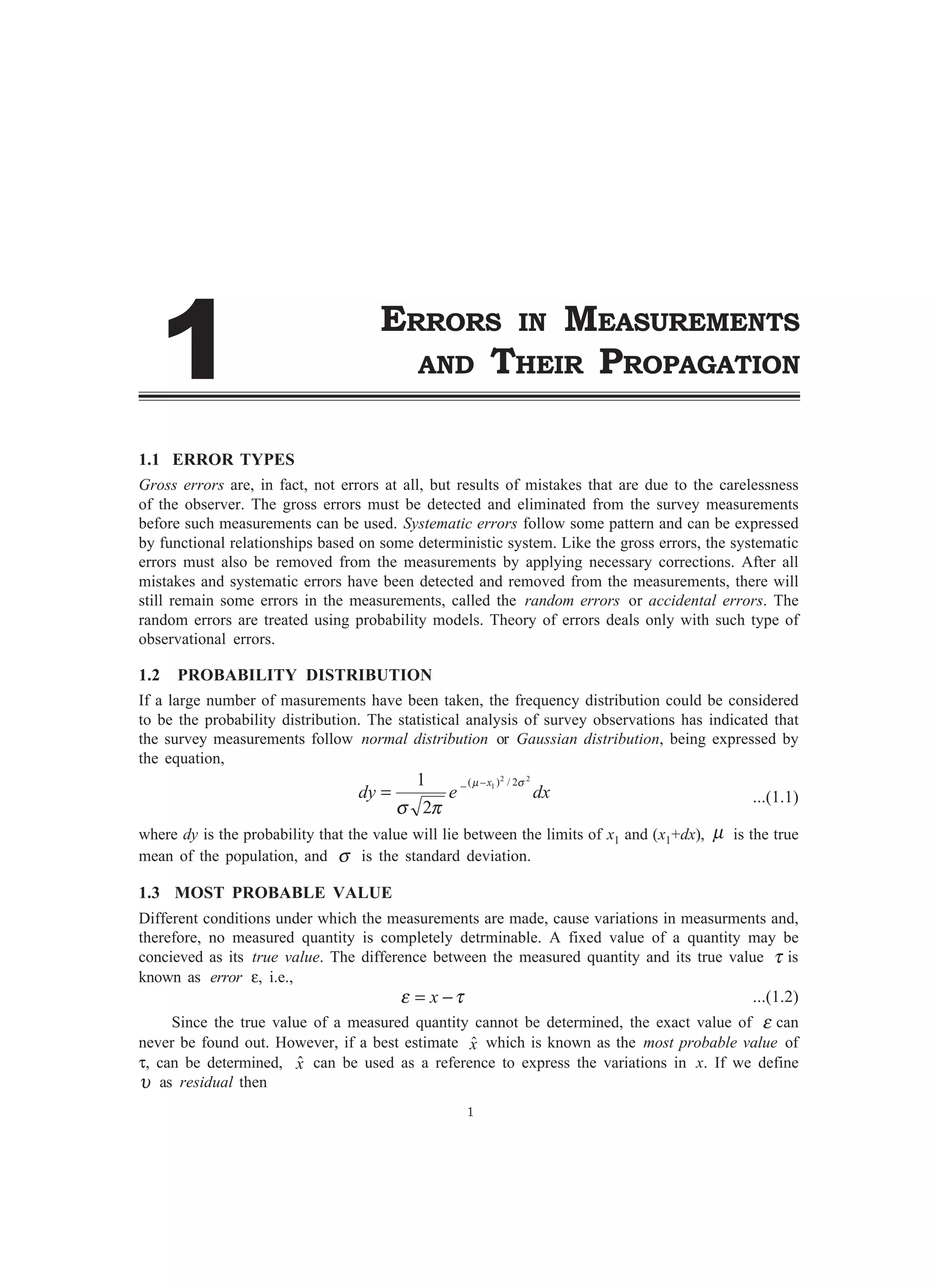
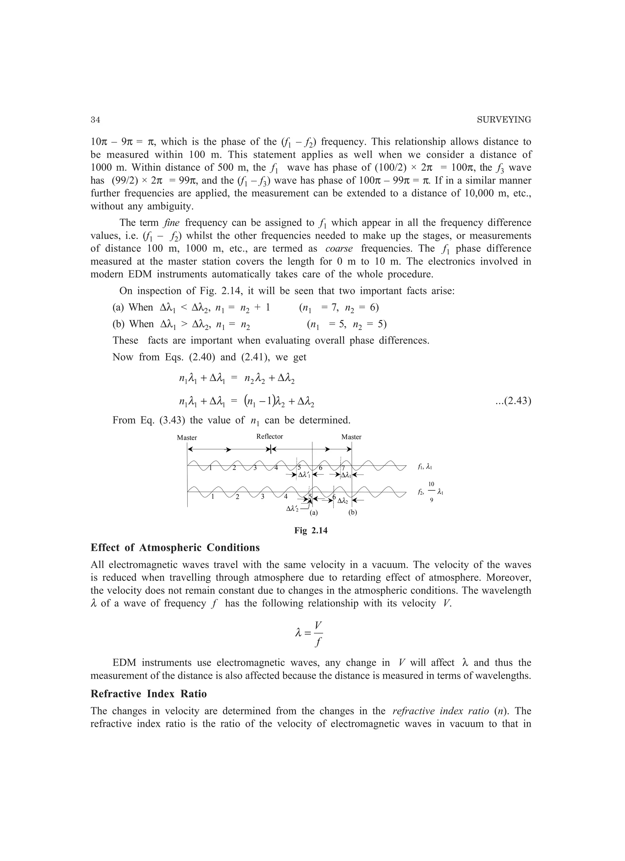
![LEVELLING 63
Section-1Section-2
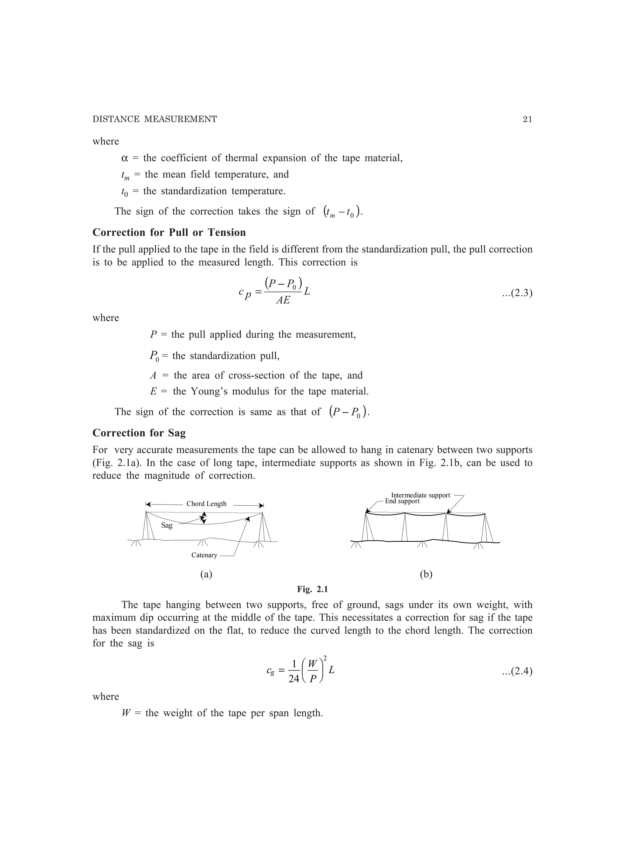
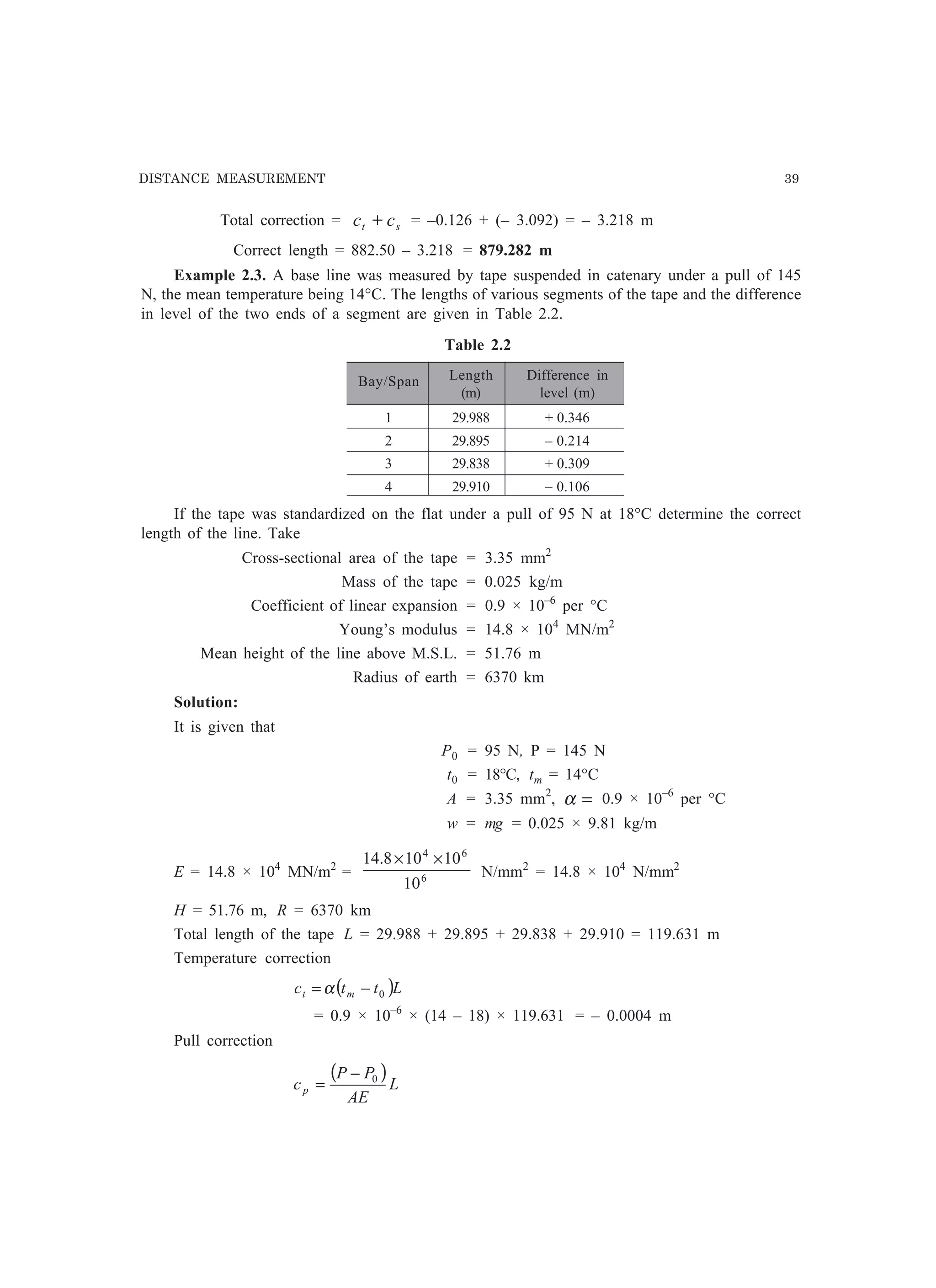
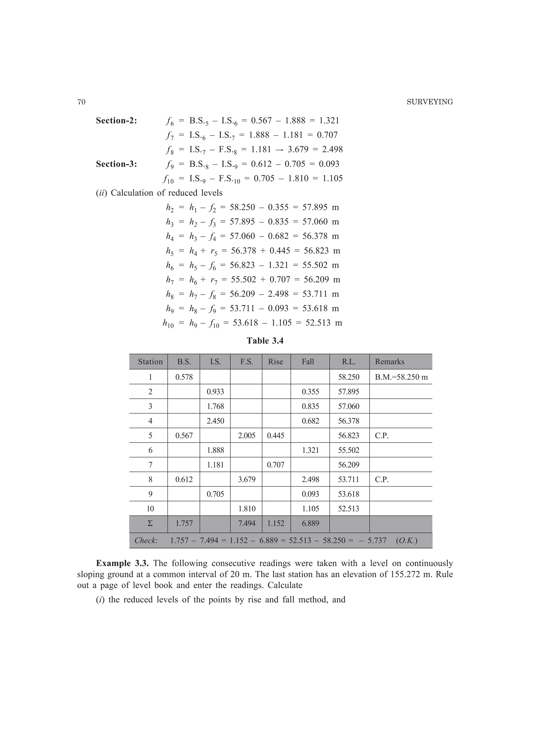
station obtains the level for a forward station. In Table 3.2, r and f indicate the rise and the fall,
respectively, assumed between the consecutive points.
Table 3.2 Rise and fall method
Station B.S. I.S. F.S. Rise Fall R.L. Remarks
A S1 hA B.M. = ha
a S2 r1 = ha = hA + r1
S1 – S2
b S3 f1 = S2 – S3 hb = ha – f1
B S5 S4 f2 = S3 – S4 hB = hb – f2 C.P.
c S6 f3 = S5 – S6 hc = hB – f3
C S7 r2 = HC = hc + r2
S6 – S7
Σ B.S. Σ F.S. Σ Rise Σ Fall
Check: Σ B.S. − Σ F.S. = Σ Rise − Σ Fall = Last R.L. − First R.L.
The arithmetic involved in reduction of the levels is used as check on the computations. The
following rules are used in the two methods of reduction of levels.
(a) For the height of instrument method
(i) Σ B.S. – Σ F.S. = Last R.L. – First R.L.
(ii) Σ [H.I. × (No. of I.S.’s + 1)] – Σ I.S. – Σ F.S. = Σ R.L. – First R.L.
(b) For the rise and fall method
Σ B.S. – Σ F.S. = Σ Rise – Σ Fall = Last R.L. – First R.L.
3.6 COMPARISON OF METHODS AND THEIR USES
Less arithmetic is involved in the reduction of levels with the height of instrument method than with
the rise and fall method, in particular when large numbers of intermediate sights is involved.
Moreover, the rise and fall method gives an arithmetic check on all the levels reduced, i.e., including
the points where the intermediate sights have been taken, whereas in the height of instrument
method, the check is on the levels reduced at the change points only. In the height of instrument
method the check on all the sights is available only using the second formula that is not as simple
as the first one.
The height of instrument method involves less computation in reducing the levels when there
are large numbers of intermediate sights and thus it is faster than the rise and fall method. The rise
and fall method, therefore, should be employed only when a very few or no intermediate sights are
taken in the whole levelling operation. In such case, frequent change of instrument position requires
determination of the height of instrument for the each setting of the instrument and, therefore,
computations involved in the height of instrument method may be more or less equal to that required
in the rise and fall method. On the other hand, it has a disadvantage of not having check on the
intermediate sights, if any, unless the second check is applied.](https://image.slidesharecdn.com/surveyingproblemsolving-150308103254-conversion-gate01/75/Surveying-problem-solving-76-2048.jpg)
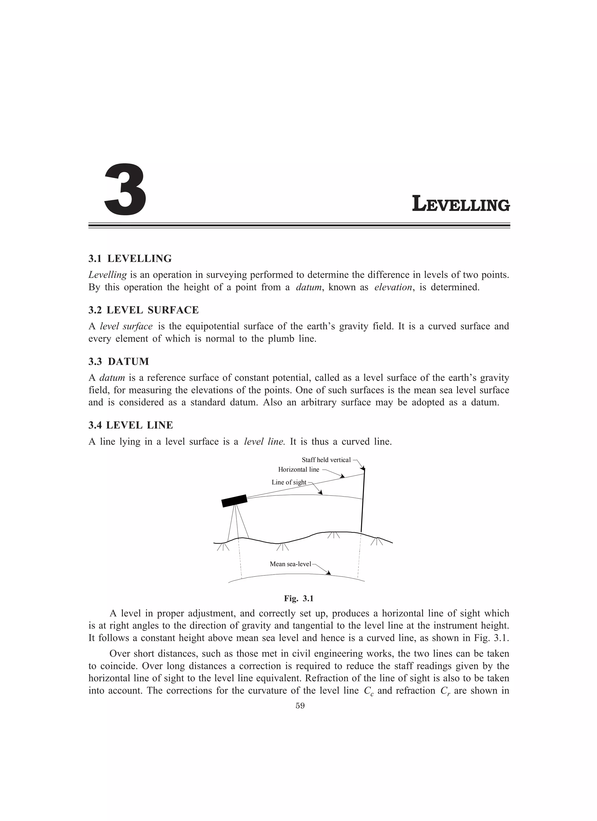
![LEVELLING 69
Section-2:
H.I.5 = h5 + B.S.5 = 56.823 + 0.567 = 57.390 m
h6 = H.I.2 – I.S.6 = 57.390 – 1.888 = 55.502 m
h7 = H.I.2 – I.S.7 = 57.390 – 1.181 = 56.209 m
h8 = H.I.2 – F.S.8 = 57.390 – 3.679 = 53.711 m
Section-3:
H.I.8 = h8 + B.S.8 = 53.711 + 0.612 = 54.323 m
h9 = H.I.8 – I.S.9 = 54.323 – 0.705 = 53.618 m
h10 = H.I.8 – F.S.10 = 54.323 – 1.810 = 52.513 m
Additional check for H.I. method: Σ [H.I. × (No. of I.S.s + 1)] – Σ I.S. – Σ F.S. = Σ R.L.
– First R.L.
[58.828 × 4 + 57.390 ´ 3 + 54.323 × 2] – 8.925 – 7.494 = 557.959 – 58.250 = 499.709 (O.K.)
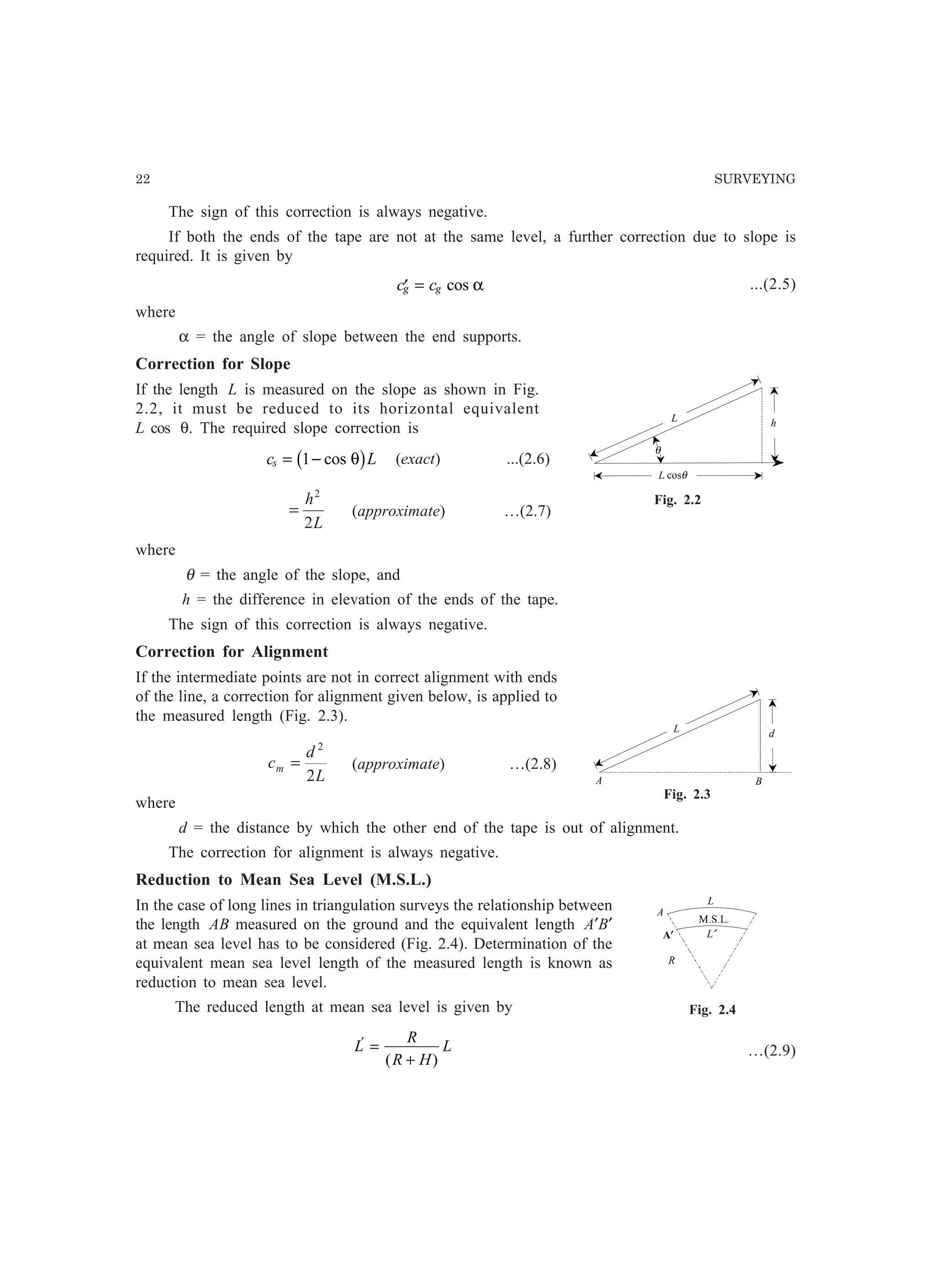
Table 3.3
Station B.S. I.S. F.S. H.I. R.L. Remarks
1 0.578 58.828 58.250 B.M.=58.250 m
2 0.933 57.895
3 1.768 57.060
4 2.450 56.378
5 0.567 2.005 57.390 56.823 C.P.
6 1.888 55.502
7 1.181 56.209
8 0.612 3.679 54.323 53.711 C.P.
9 0.705 53.618
10 1.810 52.513
Σ 1.757 8.925 7.494 557.956
Check: 1.757 – 7.494 = 52.513 – 58.250 = – 5.737 (O.K.)
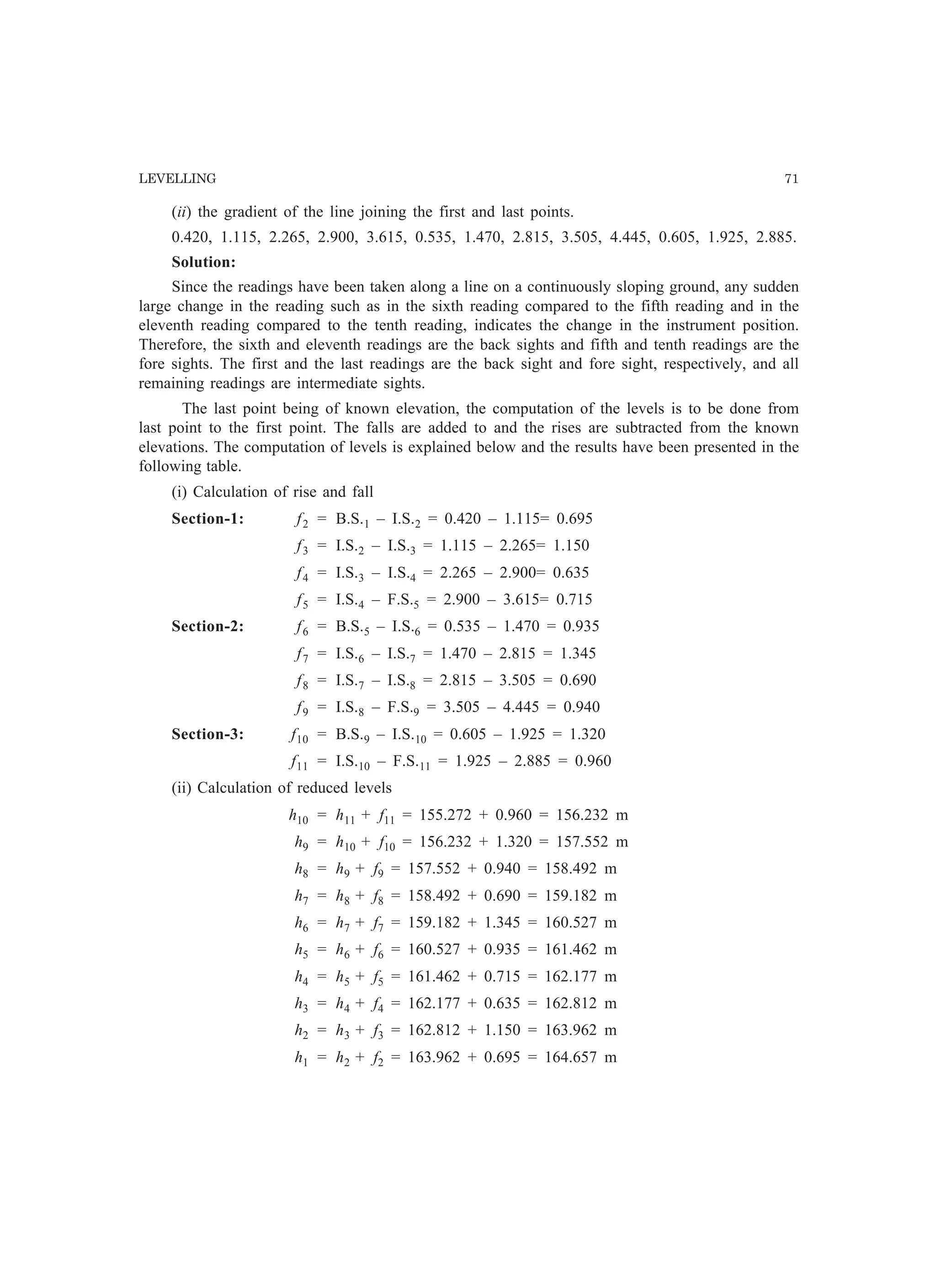
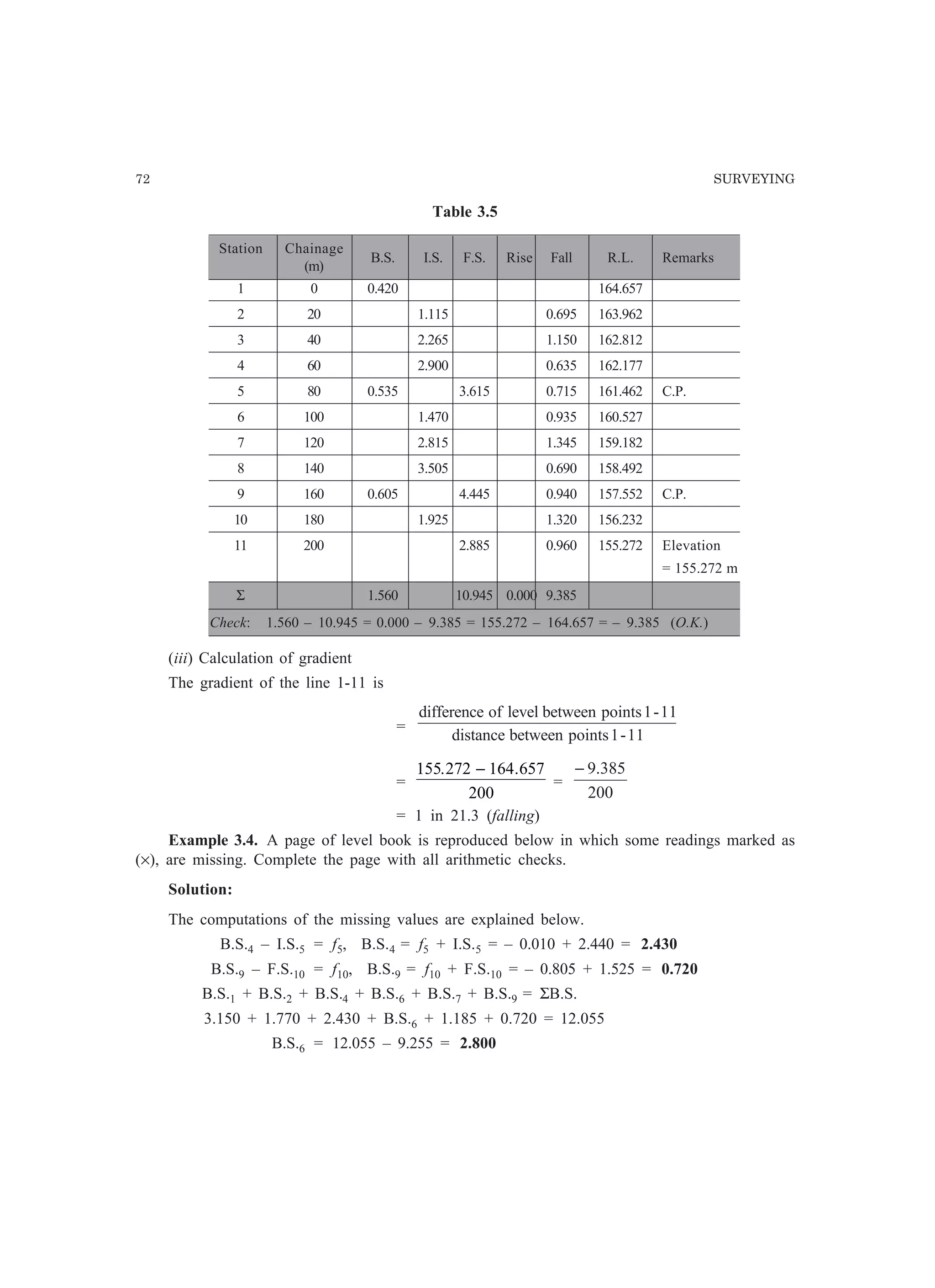
Example 3.2. Reduce the levels of the stations from the readings given in the Example 3.1 by
the rise and fall method.
Solution:
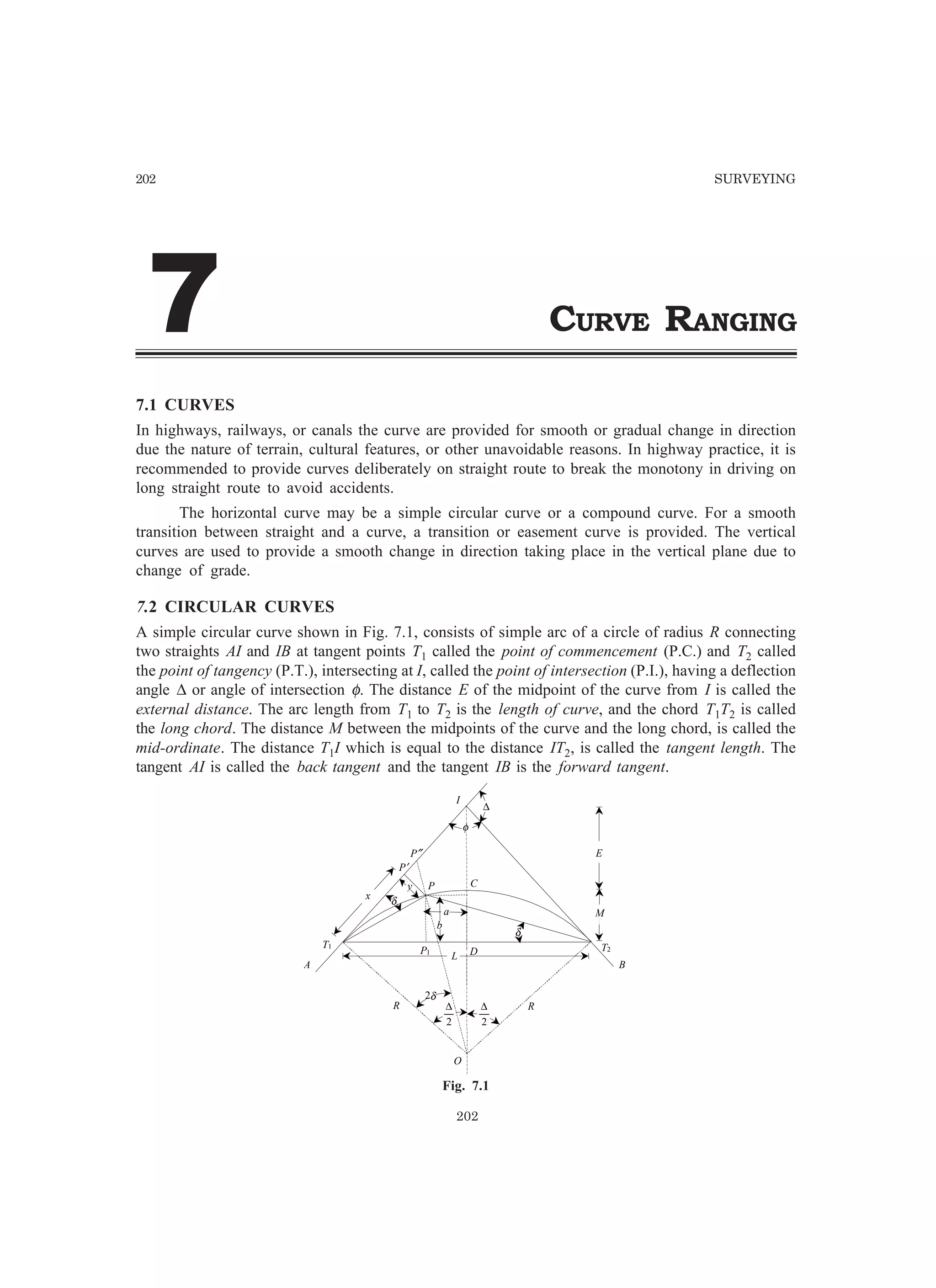
Booking of the readings for reducing the levels by rise and fall method is same as explained
in Example 3.1. The computations of the reduced levels by rise and fall method is given below and
the results are tabulated in the table. In the following computations, the values of B.S., I.S., Rise
(r), Fall (f ), etc., for a particular station have been indicated by its number or name.
(i) Calculation of rise and fall
Section-1: f2 = B.S.1 – I.S.2 = 0.578 – 0.933 = 0.355
f3 = I.S.2 – I.S.3 = 0.933 – 1.768 = 0.835
f4 = I.S.3 – I.S.4 = 1.768 – 2.450 = 0.682
r5 = I.S.4 – F.S.5 = 2.450 – 2.005 = 0.445](https://image.slidesharecdn.com/surveyingproblemsolving-150308103254-conversion-gate01/75/Surveying-problem-solving-82-2048.jpg)
![124 SURVEYING
5.5 LEAST SQUARES METHOD OF CORRELATES
Correlates are the unknown multipliers used to determine the most probable values of unknown
parameters which are the errors (or the corrections) considered directly. The number of correlates
is equal to the number of condition equations, excluding the one imposed by the least squares
principle. The method of determining the most probable values has been explained in Example 5.6.
5.6 METHOD OF DIFFERENCES
If the normal equations involve large numbers, the solution of simultaneous equations becomes very
laborious. The method of differences simplifies the computations. In this method, the observation
equations are written in terms of the quantity whose most probable values is to be determined by
least squares method. The solution of Example 5.8 is based on this method.
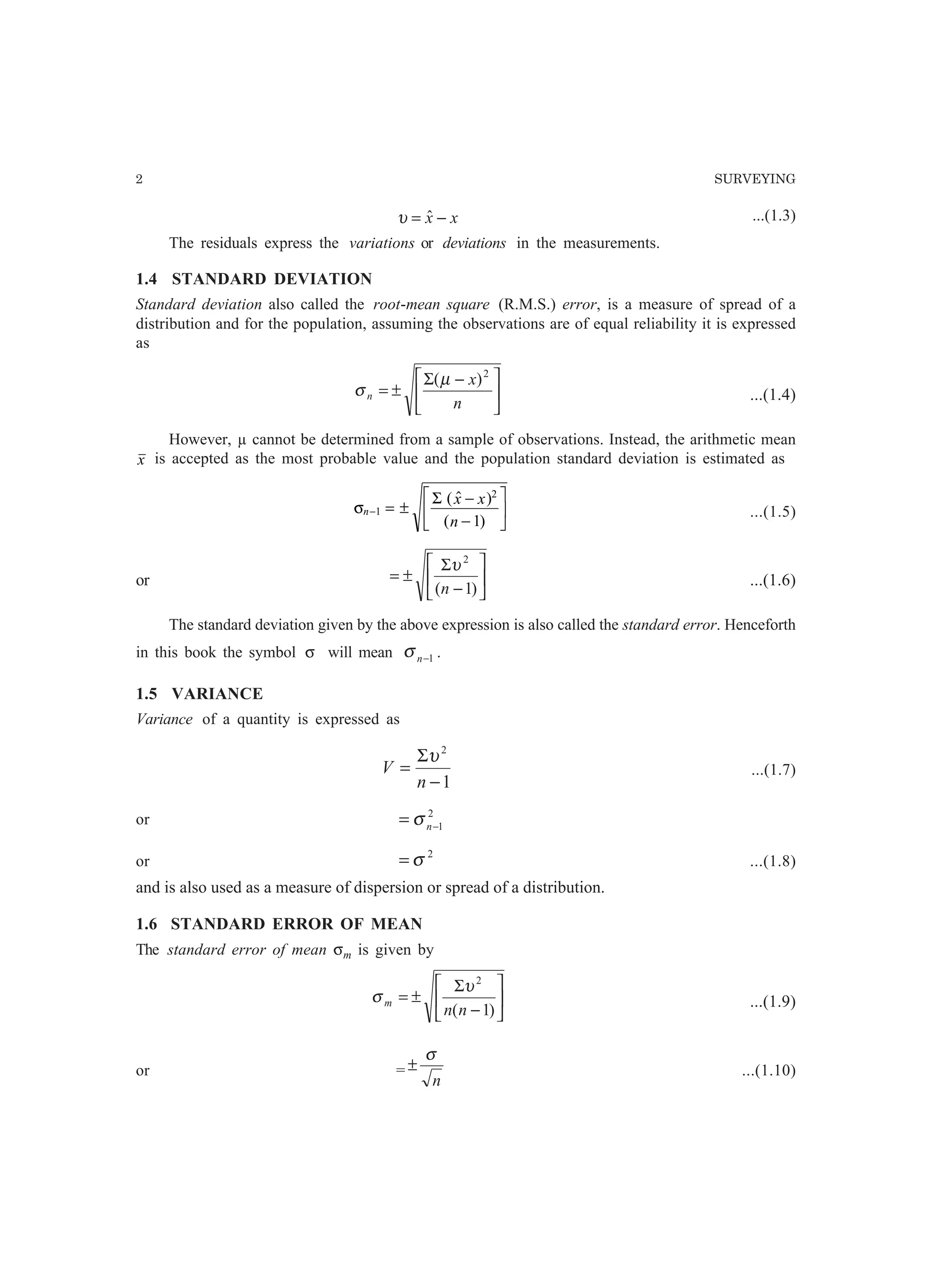
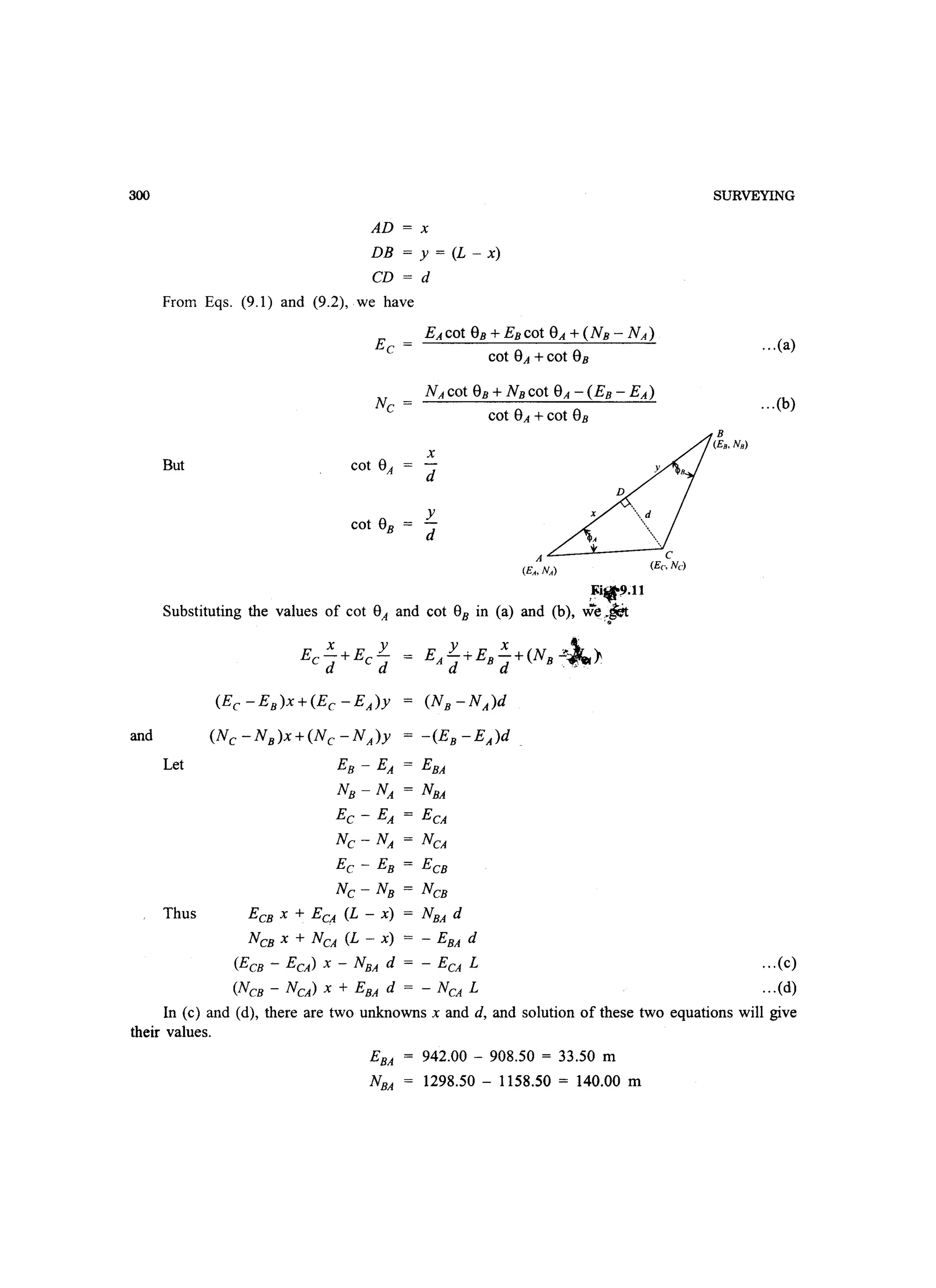
5.7 METHOD OF VARIATION OF COORDINATES
In the method of variation of coordinates, provisional coordinates are allocated to points requiring
adjustment. The amount of displacement for the adjustment is determined by the method of least
squares.
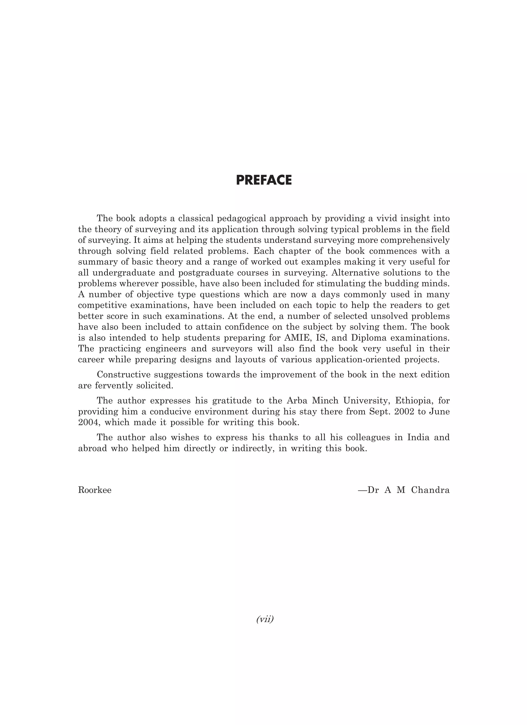
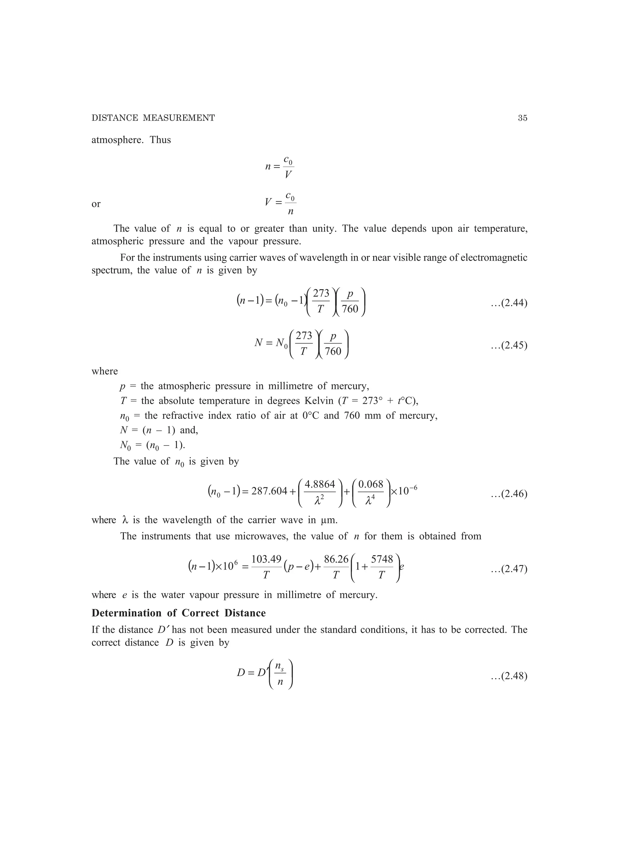
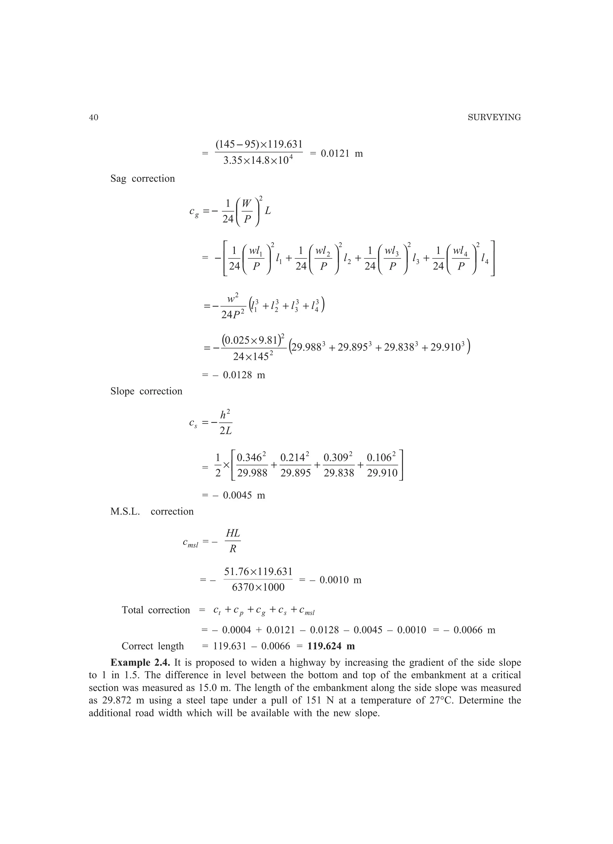
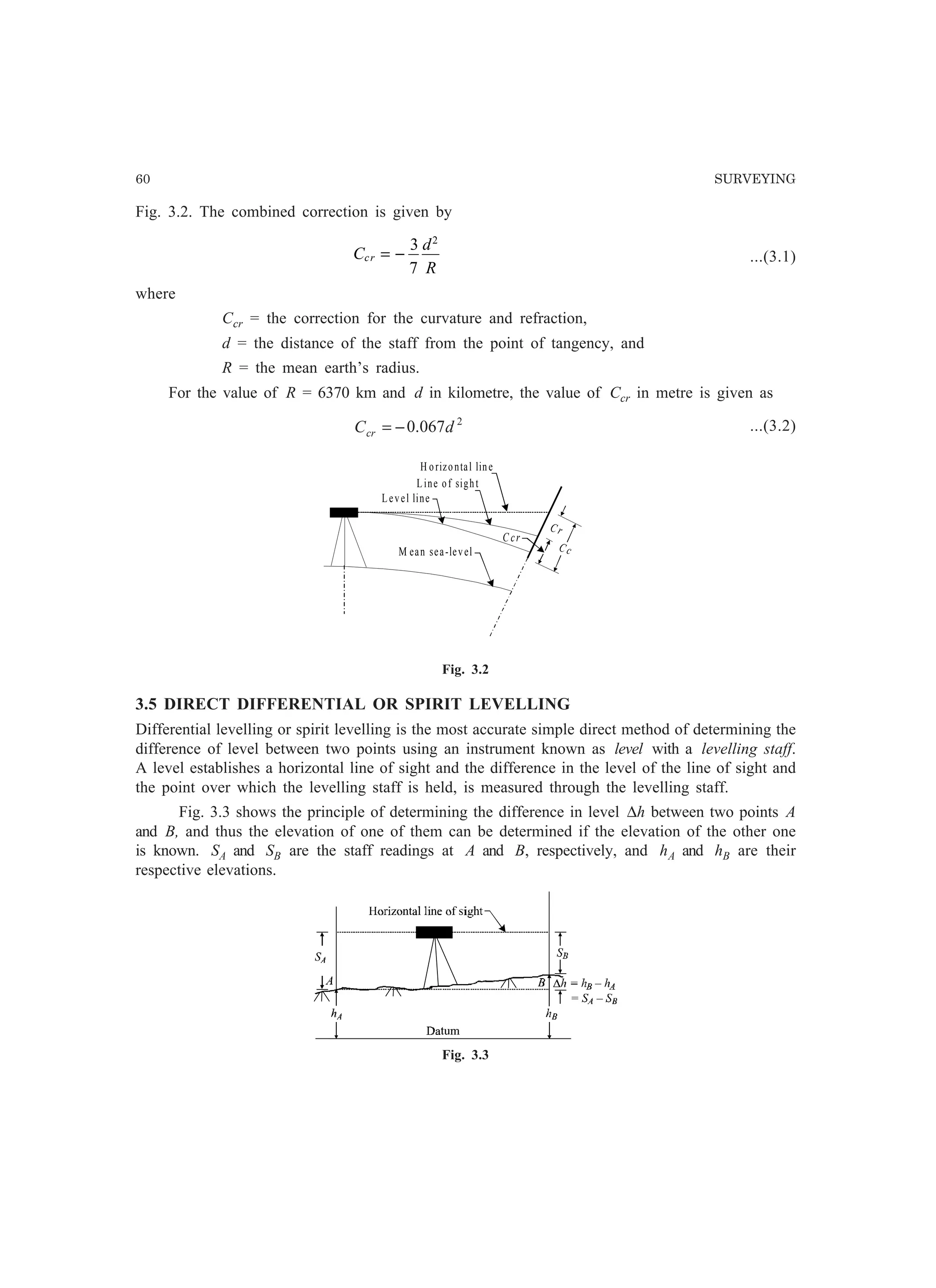
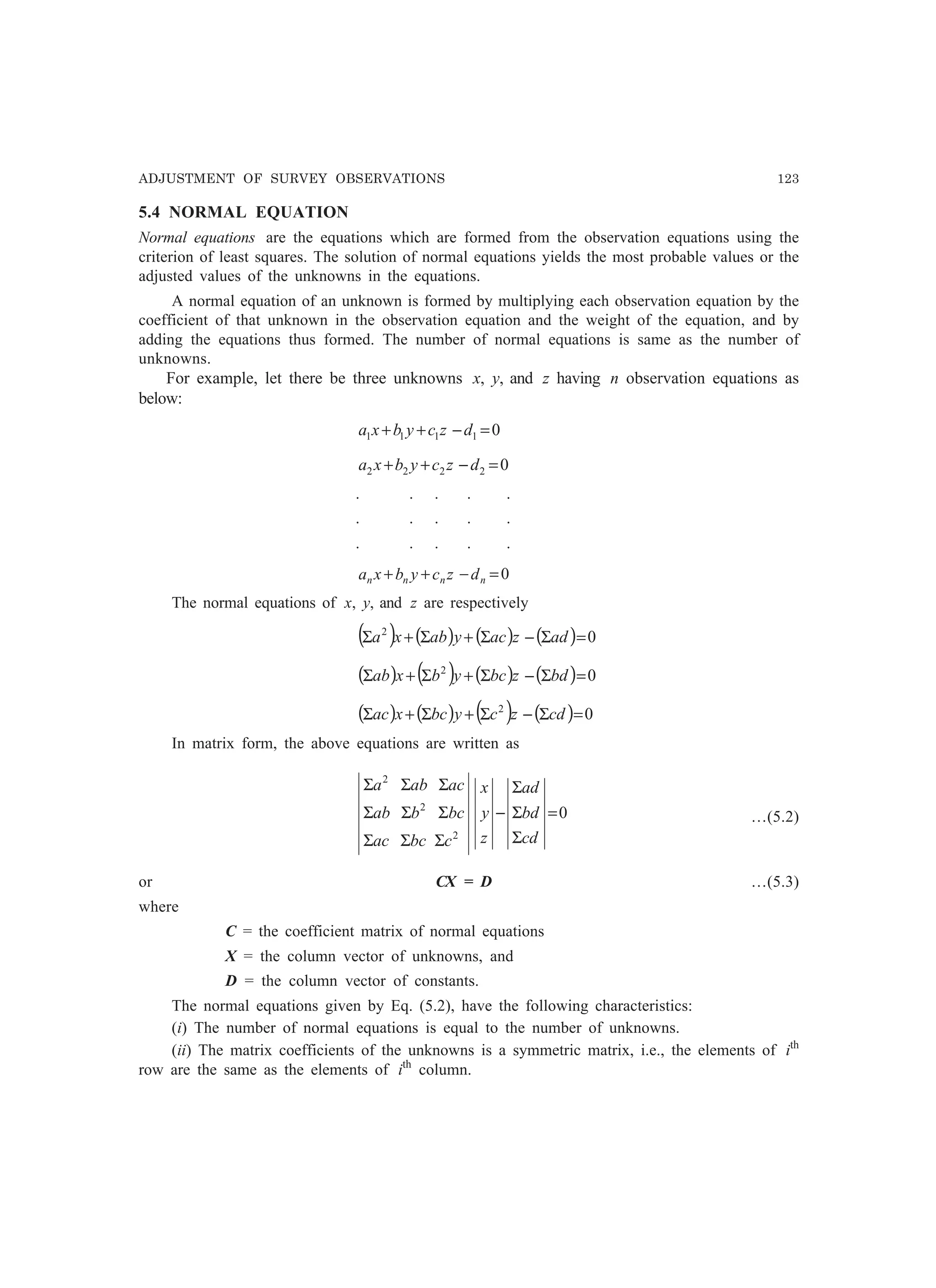
In Fig 5.1, there are two points A and B having coordinates (xA, yA) and (xB, yB), respectively,
from where the observations were made on the point C, whose coordinates are to be determined.
Let the provisional coordinates assigned to C be (xC′, yC′ ) and
the bearing of AC = θAC
the bearing of BC = θBC
the length of AC = lAC
the length of BC = lBC
the angle ACB = α
The length of AC is given by
222
)()(
ACACAC
yyxxl −′+−′=
By differentiating the above equation, we get
[ ]AACAACACCAC
AC
AC
dyyydxxx
c
dyyydxxx
l
dl )()()()(
1
−′−−′−−′+−′= …(5.4)
where dlAC is the displacement in lAC due to small displacements dxC, dxA, dyC, and dyA in C and
A, respectively.
The bearing of AC is given by
AC
AC
AC
yy
xx
−′
−′
=θtan …(5.5)
The change dθAC in the bearing due to the displacements dxC, dxA, dyC, and dyA, is
[ ]AACAACACCAC
AC
AC
dyxxdxyy
c
dyxxdxyy
l
d )()()()(
1
2
−′+−′−−′−−′=θ ...(5.6)
α
lAC
θ1
A
N
B
N
C
lBC
θ2
Fig. 5.1](https://image.slidesharecdn.com/surveyingproblemsolving-150308103254-conversion-gate01/75/Surveying-problem-solving-137-2048.jpg)
![ADJUSTMENT OF SURVEY OBSERVATIONS 125
Similar expressions can be obtained for BC and then the change in the angle ACB can be
related to dθAC and dθBC. Using the method of least squares, the displacements dx and dy in the
points can be determined. Residuals υ can be derived in the form
υ = O – C – dγ
where
O = the observed value of quantity, i.e., length, bearing, or angle,
C = the calculated value of that quantity from the coordinates, and
dγ = the change in that quantity due the displacements of the respective points.
The best value of the quantity will be C + dγ.
5.8 GENERAL METHOD OF ADJUSTING A POLYGON WITH A CENTRAL
STATION (By The Author)
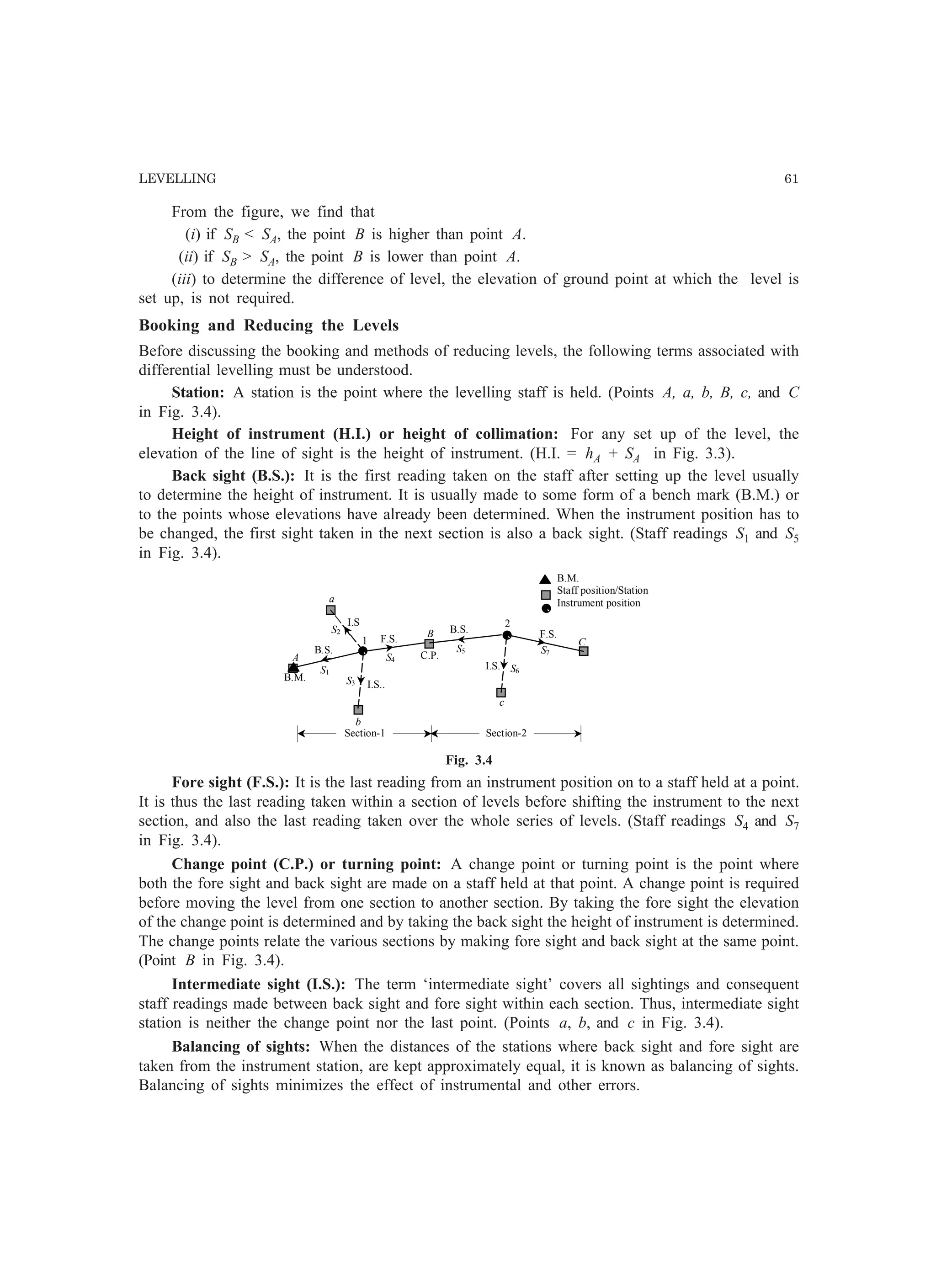
Let a polygon with a central station O has n sides and the observed angles be θ1, θ2, …., θ3n as
shown in Fig. 5.2. The total number of angles observed in this polygon will be 3n with n angles
around the central station.
The computations are done step-wise as explained below.
Step-1: Determine the total corrections for (i) each triangle, (ii) the central station and (iii)
the side conditions
(i) C1 = 180° – (θ1 + θ2 + θ2n+1)
C2 = 180° – (θ3 + θ4 + θ2n+2)
C3 = 180° – (θ5 + θ6 + θ2n+3)
. . .
. . .
Cn = 180° – (θ2n–1 + θ2n + θ3n)
(ii) Cn+1 = 360° – (θ2n+1 + θ2n+2 +…..+ θ3n)
(iii) Cn+2 = – [log sin(odd angles) – log sin(even angles)] × 106
for angles (θ1, θ2…θ2n).
Calculate log sin of the angles using pocket calculator and ignore the negative sign of the
values.
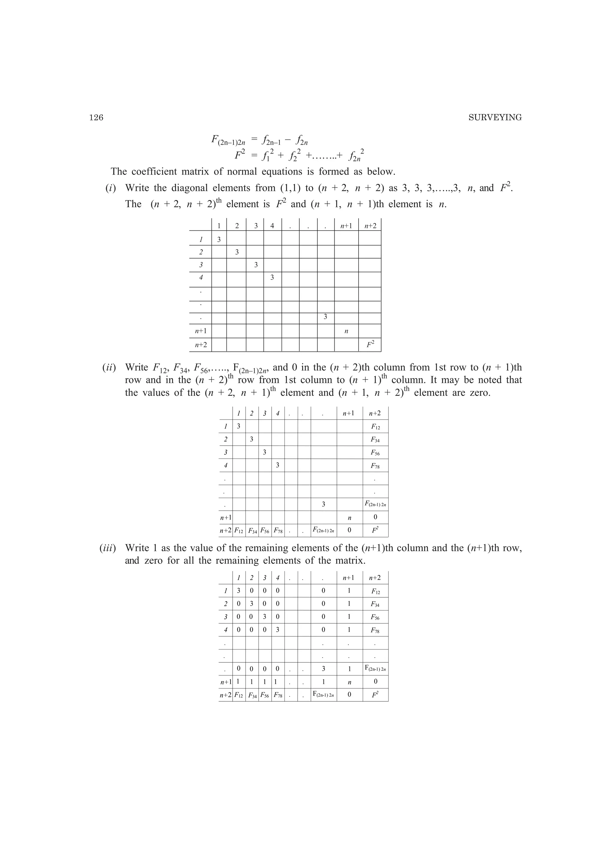
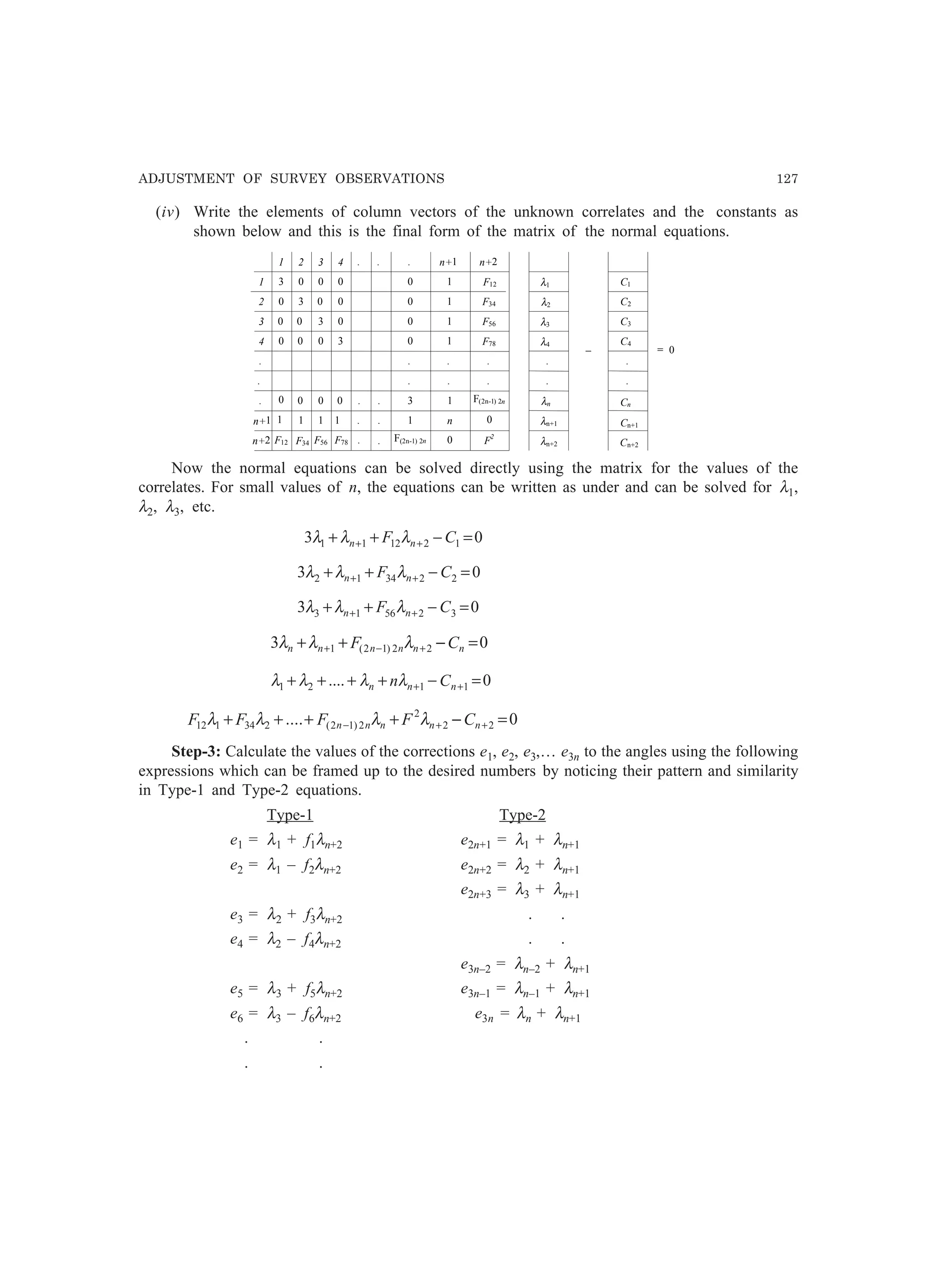
Step-2: Framing the normal equations of the correlates
There will be (n + 2) correlates and the normal equations for the correlates will be written in
matrix form. The size of the coefficient matrix will be (n + 2) × (n + 2). The column vectors of
correlates and constants will have (n + 2) elements.
Let f1, f2, f3, etc., = the differences for 1″ of log sin of the angles × 106
F12 = f1 – f2
F34 = f3 – f4
F56 = f5 – f6
. .
. .
θ1
θ2
θ3
θ4
θ5 θ6
θ2n-1
θ2n
θ3n
θ2n+1
θ2n+2
θ2n+3
Fig. 5.2](https://image.slidesharecdn.com/surveyingproblemsolving-150308103254-conversion-gate01/75/Surveying-problem-solving-138-2048.jpg)
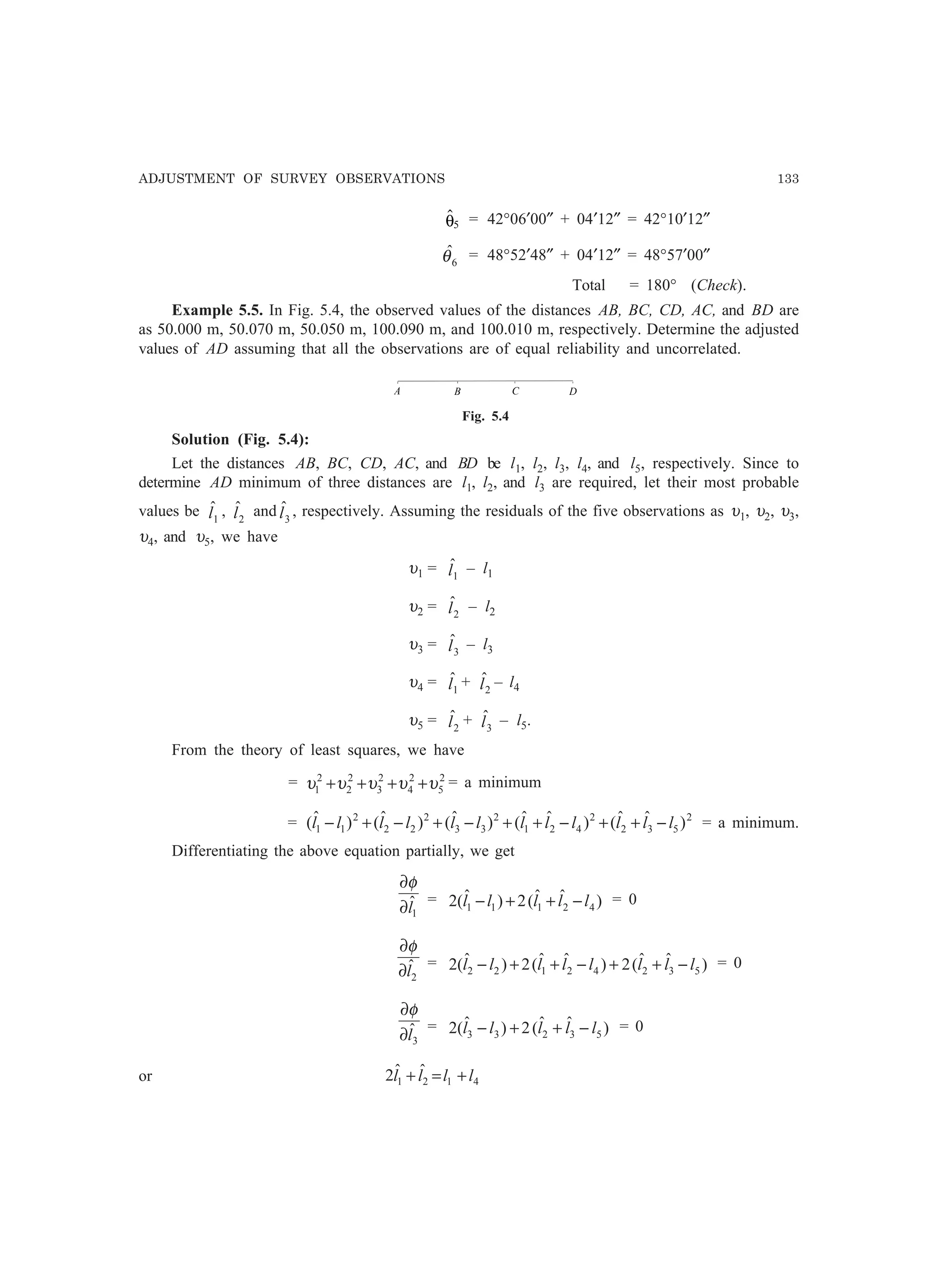
![134 SURVEYING
542321
ˆˆ3ˆ llllll ++=++
5332
ˆˆ2 llll +=+
or 21
ˆˆ2 ll + = 50.000 + 100.090 = 150.090 …(a)
321
ˆˆ3ˆ lll ++ = 50.070 + 100.090 + 10.010 = 250.170 …(b)
32
ˆˆ2 ll + = 50.050 + 100.010 = 150.060 …(c)
From Eq. (c), we get 3
ˆl =
2
ˆ060.150 2l−
…(d)
From Eq. (a), we get 2
ˆl = 1
ˆ2090.150 l− …(e)
Now substituting the values of 2
ˆl and 3
ˆl in Eq. (b), we get
170.250)]ˆ2090.150(060.150[
2
1
)ˆ2090.150(3ˆ
111 =−−×+−×+ lll
4 1
ˆl = 200.085
1
ˆl = 50.022 m
From Eq. (e), we get 2
ˆl = 150.090 – 2 × 50.022
= 50.046 m
From Eq. (d), we get 3
ˆl =
2
046.5060150.0 −
= 50.007 m
Thus the adjusted distance AD = 50.022 + 50.046 + 50.007
= 150.075 m.
Example 5.6. Find the least square estimate of the quantity x from the following data:
x (m) Weight
2x = 292.500 ω1 = 1
3x = 438.690 ω2 = 2
4x = 585.140 ω3 = 3
Solution:
Let xˆ = the least square estimate of x and](https://image.slidesharecdn.com/surveyingproblemsolving-150308103254-conversion-gate01/75/Surveying-problem-solving-147-2048.jpg)

![140 SURVEYING
[(– 1) × (– 1)Q + (– 1) × (0)R + (– 1) × (0)S + (– 1) × 143.794] + [(+ 1) × (+ 1)Q
+ (+ 1) × (0)R + (+ 1) × (–1)S + (+ 1) × (– 5.133)] + [(– 1) × (– 1)Q + (– 1) × (+ 1)
R + (– 1) × (0)S + (– 1) × (– 23.521)] = 0
or 3Q – R – S = 125.406 …(e)
To obtain the normal equation for R
The coefficients of R appear in fourth, fifth and sixth lines. Multiply the fourth line by (+ 1),
the fifth line by (+ 1) and the sixth line by (+ 1), and add them. The result is
[(+ 1) × (– 1)Q + (+ 1) × (+ 1)R + (+ 1) × (0)S + (+ 1) × (–23.521)] + [(+ 1) × (0)Q
+ (+ 1) × (+ 1)R + (+ 1) × (–1)S + (+ 1) × (– 28.639)] + [(+ 1) × (0)Q + (+ 1) × (+ 1)
R + (+ 1) × (0)S + (+ 1) × (– 167.295)] = 0
or – Q +3R – S = 219.455 …(f)
To obtain the normal equation for S
The coefficients of S appear in second, third and fifth lines. Multiply the second line by (– 1),
the third line by (– 1) and the fifth line by (– 1), and add them. The result is
[(– 1) × (+ 1)Q + (– 1) × (0)R + (– 1) × (– 1)S + (– 1) × (– 5.133)] + [(– 1) × (0)Q
+ (– 1) × (0)R + (– 1) × (–1)S + (– 1) × 138.652] + [(– 1) × (0)Q + (– 1) × (+ 1)
R + (– 1) × (– 1)S + (– 1) × (– 28.639)] = 0
or – Q – R + 3S = 104.880. …(g)
Comparing the Eqs. (e), (f) and (g) with Eqs. (d), we find that they are same. It will be realized
that we have automatically carried out the partial differentiation of φ demanded by the principle of
least squares.
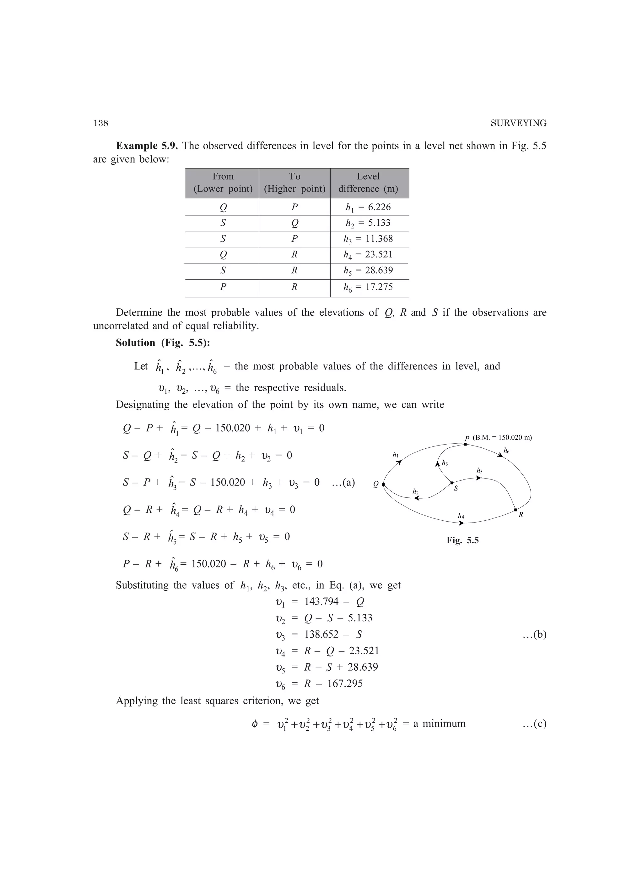
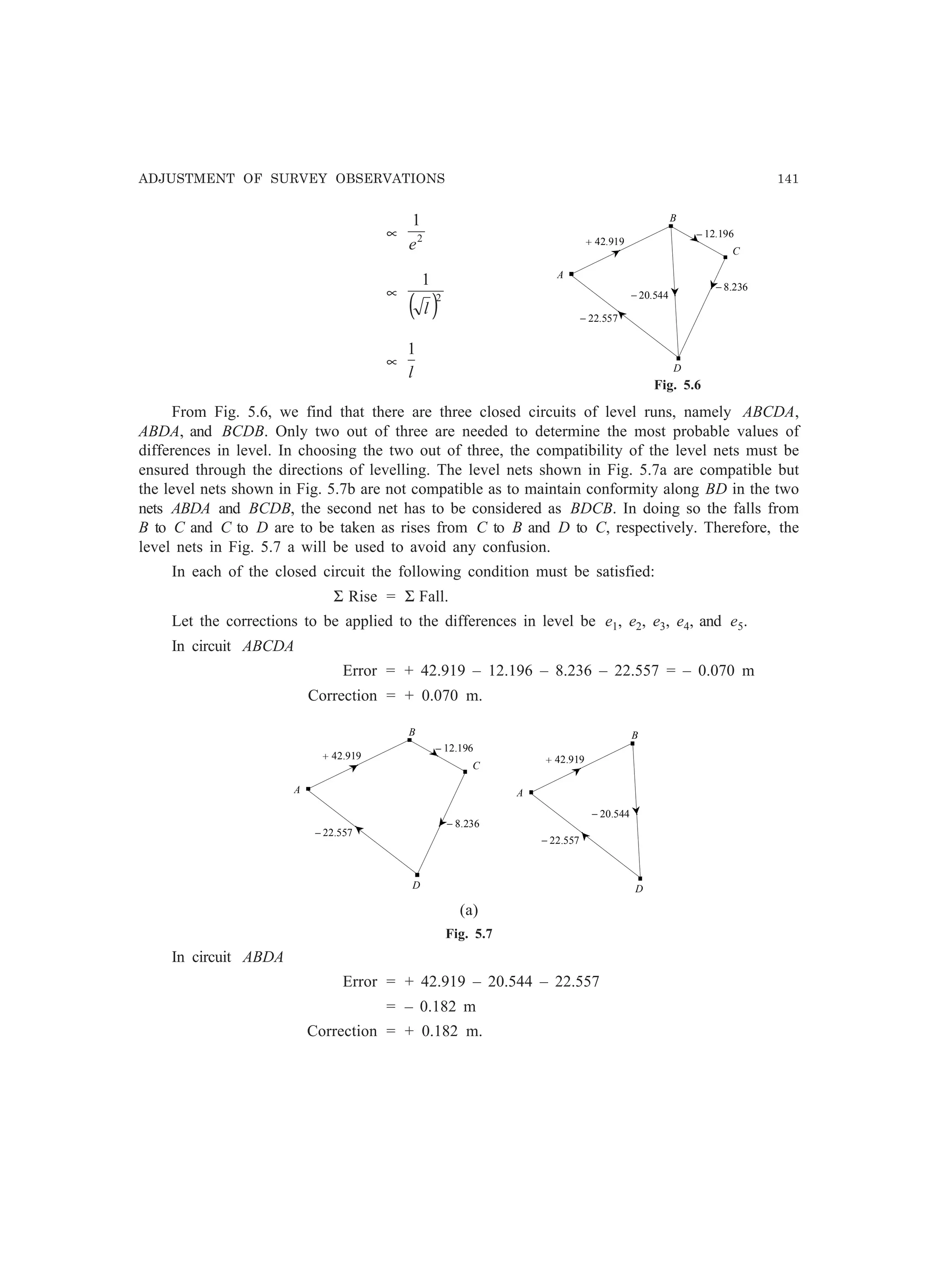
Example 5.10. Determine the least square estimates of the levels of B, C, and D from the
following data for the level net shown in Fig. 5.6. The level difference for the line A to B is the
mean of the two runs, all other lines being observed once only.
Line
Length Level difference (m)
(km) Rise (+) Fall (–)
A to B 22 42.919 –
B to C 12 – 12.196
B to D 25 – 20.544
C to D 22 – 8.236
D to A 32 – 22.557
Solution (Fig. 5.6):
Assuming the distance being equal for the back sights and fore sights, the accidental errors may
be taken as proportional to (number of instrument stations ) and hence proportional to
(length of line ). Accordingly, the weights of the observations can be taken as inversely proportional
to the square of the errors and, therefore, can be taken as the reciprocal of the length of the line, i.e.,](https://image.slidesharecdn.com/surveyingproblemsolving-150308103254-conversion-gate01/75/Surveying-problem-solving-153-2048.jpg)
![ADJUSTMENT OF SURVEY OBSERVATIONS 149
The signs of the corrections C3 to angles θ3, θ4, θ7, and θ8 are determined as below:
Since the sum of θ3 and θ4 is more than the sum of θ7 and θ8, the correction to each θ3 and
θ4, is – 2″ and the correction to each θ7 and θ8, is +2″.
Therefore the corrected angles are
θ3 = 33°52′59″ – 2″ = 33°52′57″
θ4 = 63°41′28″ – 2″ = 63°41′26″
θ7 = 50°10′47″ + 2″ = 50°10′49″
θ8 = 47°23′32″ + 2″ = 47°23′34″
θ3 + θ4 = 97°34′23″ = θ7 + θ8 (Check).
Satisfying the condition (iv)
The following computations involve the values of (log sin) of the angles which were determined
using a log table before the inception of digital calculators. As the students now, will be using the
calculators, the method of determining the values of (log sin θ) and other quantities using a
calculator has been used here.
The corrections to the individual angles for satisfying the condition (iv), is given as
cn = 2
f
fn
∑
δ
seconds …(a)
where
fn = the difference 1″ for log sinθn multiplied by 106
, i.e.,
[log sin(θn + 1″) – log sin θn] × 106
,
d = [Σ log sin(odd angle) – Σ log sin(even angle)]
× 106
ignoring the signs of Σ log sin(odd angle)
and Σ log sin (even angle), and
Σf 2
= the sum of squares of f1, f2, f3, etc., i.e.,
22
3
2
2
2
1 ....... nffff ++++ .
The sign of the corrections Cn is decided as below.
If Σ log sin(odd angle) Σ log sin(even angle), the corrections for odd angles will be positive
and for the even angles negative and vice-versa.
Calculating the values of log sin(odd angle)’s, ignoring the signs
log sin θ1 = log sin (43°48′31″) = 0.1597360, f1 = 22
log sin θ3 = log sin (33°52′57″) = 0.2537617, f3 = 31
log sin θ5 = log sin (49°20′42″) = 0.1199607, f5 = 18
log sin θ7 = log sin (50°10′49″) = 0.1146031, f7 = 18
Σ log sin(odd angle) = 0.6480615](https://image.slidesharecdn.com/surveyingproblemsolving-150308103254-conversion-gate01/75/Surveying-problem-solving-162-2048.jpg)
![150 SURVEYING
Calculating the values of log sin(even angle)’s, ignoring the signs
log sin θ2 = log sin (38°37′06″) = 0.2047252, f2 = 26
log sin θ4 = log sin (63°41′26″) = 0.0474917, f4 = 10
log sin θ6 = log sin (33°04′55″) = 0.2629363, f6 = 32
log sin θ8 = log sin (47°23′34″) = 0.1331152, f8 = 19
Σ log sin (even angle) = 0.6482684
Therefore, δ = [Σ log sin (odd angle) – Σ log sin (even angle)] × 106
= (0.6480615 – 0.6482684) × 106
= 2069 (ignoring the sign)
and Σf 2
= 222
+ 262
+ 312
+ 102
+ 182
+ 322
+ 182
+ 192
= 4254.
Since Σ log sin (odd angle) Σ log sin (even angle) the corrections c1, c3, c5, and c7 will be
negative, and c2, c4, c6, and c8 will be positive.
Thus c1 = 22 ×
4254
2069
= – 10.7″; c5 = 18 ×
4254
2069
= – 8.8″
c2 = 26 ×
4254
2069
= + 12.6″; c6 = 32 ×
4254
2069
= + 15.6″
c3 = 31 ×
4254
2069
= – 15.1″; c7 = 18 ×
4254
2069
= – 8.8″
c4 = 10 ×
4254
2069
= + 4.9″; c8 = 19 ×
4254
2069
= + 9.2″.
Therefore the adjusted values of the angles are
θ1 = 43°48′31″ – 10.7″= 43°48′′′′′20.3″″″″″
θ2 = 38°37′06″ + 12.6″ = 38°37′′′′′18.4″″″″″
θ3 = 33°52′57″ – 15.1″= 33°52′′′′′41.9″″″″″
θ4 = 63°41′26″ + 4.9″ = 63°41′′′′′30.9″″″″″
θ5 = 49°20′42″ – 8.8″ = 49°20′′′′′33.2″″″″″
θ6 = 33°04′55″ + 15.6″ = 33°05′′′′′10.6″″″″″
θ7 = 50°10′49″ – 8.8″ = 50°10′′′′′40.2″″″″″
θ8 = 47°23′34″ + 9.2″ = 47°23′′′′′43.2″″″″″
Total = 359°59′58.7″ (Check).
Since there is still an error of 1.3″, if need be one more iteration of all the steps can be done
to get better most probable values of the angles. Alternatively, since the method is approximate, one
can add
8
3.1 ′′
= 0.163″ to each angle and take the resulting values as the most probable values.](https://image.slidesharecdn.com/surveyingproblemsolving-150308103254-conversion-gate01/75/Surveying-problem-solving-163-2048.jpg)
![ADJUSTMENT OF SURVEY OBSERVATIONS 151
Thus, θ1 = 43°48′20.3″ + 0.163″ = 43°48′20.463″
θ2 = 38°37′18.6″ + 0.163″ = 38°37′18.763″
θ3 = 33°52′41.9″ + 0.163″ = 33°52′42.063″
θ4 = 63°41′30.9″ + 0.163″ = 63°41′31.063″
θ5 = 49°20′33.2″ + 0.163″ = 49°20′33.363″
θ6 = 33°05′10.6″ + 0.163″ = 33°05′10.763″
θ7 = 50°10′40.2″ + 0.163″ = 50°10′40.363″
θ8 = 47°23′43.2″ + 0.163″ = 47°23′43.363″
Total = 360°00′00.204″ (Check).
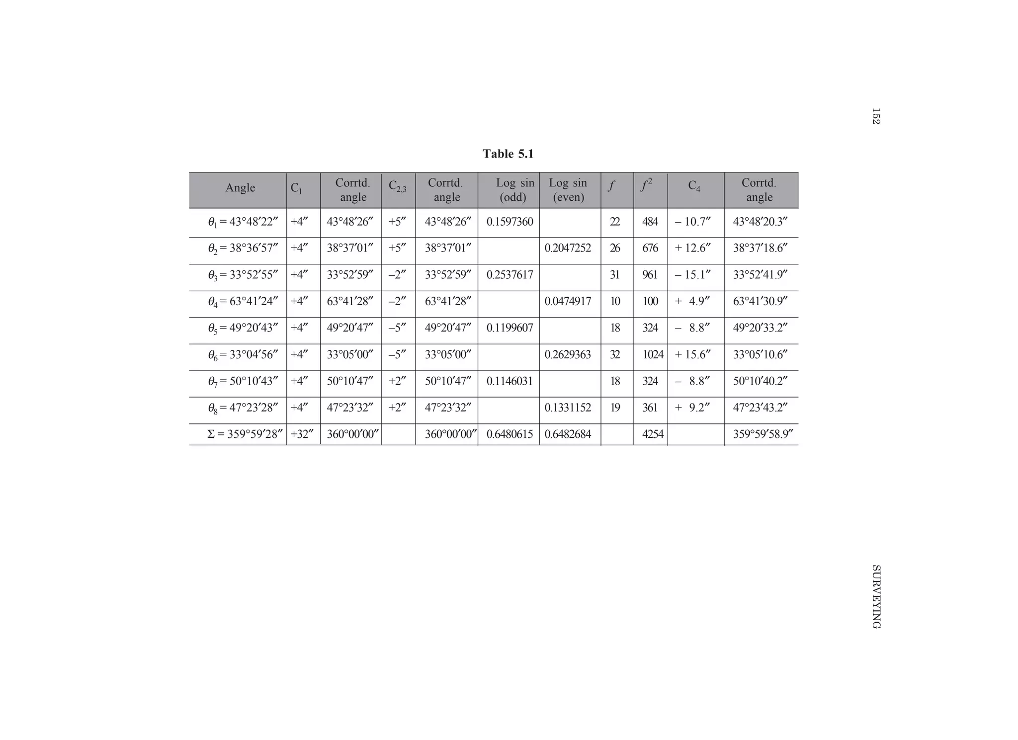
For systematic computations, the computations may be done in tabular form as given in
Table 5.1.
(b) Rigorous method
Let the corrections to the angles be e1, e2,......, e8 then from the conditions to be satisfied, we
get
e1 + e2 + e3 + e4 + e5 + e6 + e7 + e8 = + 32″ …(a)
e1 + e2 – e5 – e6 = 82°25′27″ – 82°25′47″ = + 20″ …(b)
e3 + e4 – e7 – e8 = 97°34′27″ – 97°34′19″ = – 8″ …(c)
f1e1 – f2e2 + f3e3 – f4e4 + f5e5 – f6e6 + f7e7 – f8e8 = –δ = –2069 …(d)
where δ = [Σ log sin (odd angle) – Σ log sin (even angle)] × 106
.
Another condition to be satisfied from least squares theory is
φ = 2
8
2
7
2
6
2
5
2
4
2
3
2
2
2
1 eeeeeeee +++++++ = a minimum. …(e)
Differentiating the Eq. (a) to (e), we get
87654321 eeeeeeee ∂+∂+∂+∂+∂+∂+∂+∂ = 0 …(f)
6521 eeee ∂−∂−∂+∂ = 0 …(g)
8743 eeee ∂−∂−∂+∂ = 0 …(h)
8877665544332211 efefefefefefefef ∂−∂+∂−∂+∂−∂+∂−∂ = 0 ...(i)
8877665544332211 eeeeeeeeeeeeeeee ∂+∂+∂+∂+∂+∂+∂+∂ = 0 …(j)
Multiplying Eqs. (f), (g), (h) and (i) by –λ1, –λ2, –λ3, and –λ4, respectively, and adding to
Eq. (j), and equating the coefficients of 321 ,, eee ∂∂∂ , etc., in the resulting equation, to zero, we
get
(e1 – λ1 – λ2 – f1λ4) = 0 or e1 = λ1 + λ2 + f1λ4
(e2 – λ1 – λ2 + f2λ4) = 0 or e2 = λ1 + λ2 – f2λ4
(e3 – λ1 – λ3 – f3λ4) = 0 or e3 = λ1 + λ3 + f3λ4
(e4 – λ1 – λ3 + f4λ4) = 0 or e4 = λ1 + λ3 – f4λ4](https://image.slidesharecdn.com/surveyingproblemsolving-150308103254-conversion-gate01/75/Surveying-problem-solving-164-2048.jpg)
![ADJUSTMENT OF SURVEY OBSERVATIONS 155
θ9 + θ10 + θ11 + θ12 = 360°
and the side condition to be satisfied is
∑ log sin (odd angle) = ∑ log sin (even angle)
or log sin θ1 + log sin θ3 + log sin θ5 + log sin θ7
= log sin θ2 + log sin θ4 + log sin θ6 + log sin θ8.
For the various notations used here and in other problems, Example 5.12 may be referred.
29°17′00″ + 28°42′00″ + 122°00′55″ – 180° = E1 = – 5″
e1 + e2 + e9 = C1 = + 5″
62°59′49″ + 56°28′01″ + 60°32′05″ – 180° = E2 = – 5″
e3 + e4 + e10 = C2 = + 5″
29°32′06″ + 32°03′54″ + 118°23′50″ – 180° = E3 = – 10″
e5 + e6 + e11 = C3 = + 10″
59°56′06″ + 61°00′54″ + 59°03′10″ – 180° = E4 = + 10″
e7 + e8 + e12 = C4 = – 10″
122°00′55″ + 60°32′05″ + 118°23′50″ + 59°03′10″ – 360° = E5 = 0″
e9 + e10 + e11 + e12 = C5 = 0″
Calculating the values of log sin (odd angle)’s, ignoring the signs
log sin θ1 = log sin (29°17′00″) = 0.3105768, f1 = 38
log sin θ3 = log sin (62°59′49″) = 0.0501309, f3 = 11
log sin θ5 = log sin (29°32′06″) = 0.3071926, f5 = 37
log sin θ7 = log sin (59°56′06″) = 0.0627542, f7 = 12
Σ log sin (odd angle) = 0.7306545
Calculating the values of log sin(even angle)’s, ignoring the signs
log sin θ2 = log sin (28°42′00″) = 0.3185566, f2 = 38
log sin θ4 = log sin (56°28′01″) = 0.0790594, f4 = 14
log sin θ6 = log sin (32°03′54″) = 0.2750028, f6 = 34
log sin θ8 = log sin (61°00′54″) = 0.0581177, f8 = 12
Σ log sin (even angle) = 0.7307365
Therefore δ = [Σ log sin (odd angle) – Σ log sin (even angle)] × 106
= (0.7306545 – 0.7307365) × 106
= E6
= – 820
or f1e1 – f2e2 + f3e3 – f4e4 + f5e5 – f6e6 + f7e7 – f8e8 = C6 = + 820.
Since there are six condition equations, there will be six correlates and the equations to
determine them using the theory of least squares, will be](https://image.slidesharecdn.com/surveyingproblemsolving-150308103254-conversion-gate01/75/Surveying-problem-solving-168-2048.jpg)
![158 SURVEYING
For θBC
xC – xB = 8533.38 – 7582.46 = 950.92 m
yC – yB = 12184.52 – 8483.29 = 3701.23 m
23.3701
92.950
tan =BCθ = 0.2569200
Computed value of θBC = 14°24′31.7″ = C
Observed value of θBC = 14°24′27″ = O
(O – C) = 14°24′27″ – 14°24′31.7″ = – 4.7″
=
206265
7.4
− = – 2.27862216 × 10⁻⁵
radians.
For lAC
lAC = [( ) ( ) ]x x y yC A C A− − −2 2
= [( . . )]4526 39 1119 762 2
−
Computed value of lAC = 4662.84 m = C
Observed value of lAC = 4663.08 m = O
(O – C) = 4663.08 – 4662.84 = + 0.24 m.
For lBC
lBC = [( ) ( ) ]x x y yC B C B− − −2 2
= [( . . )]950 92 3701 232 2
−
Computed value of lBC = 3821.43 m = C
Observed value of lBC = 3821.21 m = O
(O – C) = 3821.21 – 3821.43 = – 0.22 m.
For angle ACB
∠ACB = Back bearing of AC – back bearing of BC
= (180° + 76°06′17.5″) – (180° + 14°24′31.7″)
Computed value of ∠ACB = 61°41′45.8″ = C
Observed value of ∠ACB = 61°41′57″ = O
(O – C) = 61°41′57″ – 61°41′45.8″ = + 11.2″.
=
206265
2.11
+ = + 5.42990813 × 10⁻⁵
radians.
(ii) Calculation of residuals υ
Since A and B are fixed points
dxA = dxB = dyA = dyB = 0.](https://image.slidesharecdn.com/surveyingproblemsolving-150308103254-conversion-gate01/75/Surveying-problem-solving-171-2048.jpg)
![ADJUSTMENT OF SURVEY OBSERVATIONS 161
Y∂
∂φ
= 2ωθ (d1 + a1X + b1Y)b1 + 2ωθ (d2 + a2X + b2Y)b2 + 2ωl
(d3 + a3X + b3Y)b3 + 2ωl (d4 + a4X + b4Y)b4 + 2ωα
(d5 + a5X + b5Y)b5 = 0
By rearranging the terms, we get
[ωθ(a2
1 + a2
2) + ωl(a2
3 + a2
4) + ωαa2
5]X + [ωθ(b1a1 + b2a2) + ωl(b3a3 + b4a4) + ωαb5a5]Y
= – [ωθ(d1a1 + d2a2) + ωl(d3a3 + d4a4) + ωαd5a5]
[ωθ(b1a1 + b2a2) + ωl(b3a3 + b4a4) + ωab5a5]X + [ωθ(b2
1 + b2
2) + ωl(b2
3 + b2
4) + ωαb2
5]Y
= – [ωθ(d1b1 + d2b2) + ωl(d3b3 + d4b4) + ωαd5b5].
The above two equations are the normal equations in X (i.e., dxC) and Y (i.e., dyc). Now
Substituting the values of a, b, d, ωθ, ωl; and ωα, we get
634.895456 dxc + 156.454114 dyc – 48.6944390 = 0
156.454114 dxc + 552.592599 dyc + 99.6361111 = 0
The above equations solve for
dxc = + 1.30213821 × 10–1
= + 0.13 m
dyc = – 2.17173736 × 10–1
= – 0.22 m.
Hence the most probable values of the coordinates of C are
Easting of C = E 8533.38 + 0.13 = E 8533.51 m
Northing of C = N 12184.52 – 0.22 = N 12184.30 m.
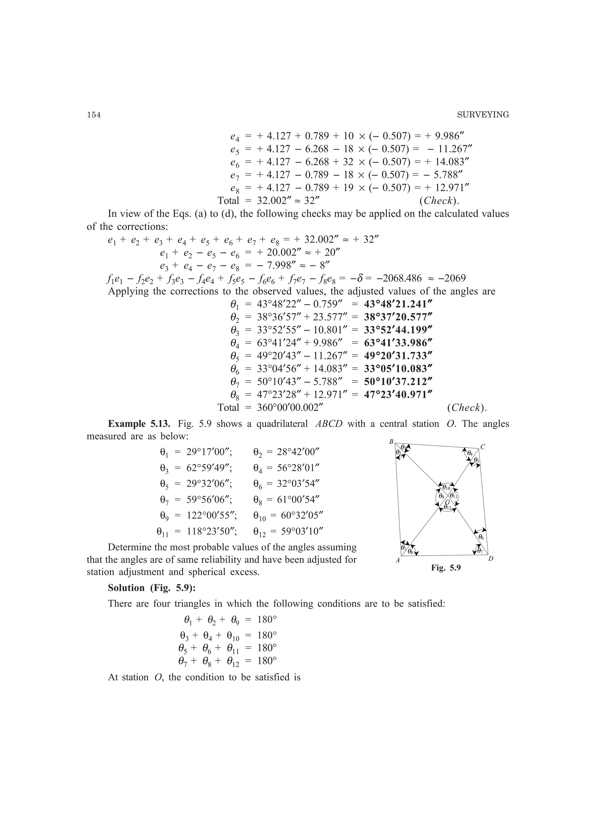
Example 5.15. A quadrilateral ABCD with a central station O is a part of a triangulation survey.
The following angles were measured, all have equal weight.
θ1 = 57°55′08″; θ2 = 38°37′27″
θ3 = 62°36′16″; θ4 = 34°15′39″
θ5 = 36°50′25″; θ6 = 51°54′24″
θ7 = 27°57′23″; θ8 = 49°52′50″
θ9 = 83°27′17″; θ10 = 83°08′06″
θ11 = 91°15′09″; θ12 = 102°09′32″.
Adjust the quadrilateral by the method of least squares.
Solution (Fig. 5.9):
This example has been solved by the general method of adjusting a polygon with a central
station discussed in Sec. 5.8.
For the given polygon
n = 4
(n + 2) = 6.
Therefore, the matrix of coefficients of normal equations will be a 6 × 6 matrix.
Step-1: Total corrections](https://image.slidesharecdn.com/surveyingproblemsolving-150308103254-conversion-gate01/75/Surveying-problem-solving-174-2048.jpg)
![162 SURVEYING
(i) C1 = 180° – (θ1 + θ2 + θ9) = + 8″
C2 = 180° – (θ3 + θ4 + θ10) = – 1″
C3 = 180° – (θ5 + θ6 + θ11) = + 2″
C4 = 180° – (θ7 + θ8 + θ12) = +15″
(ii) C5 = 360° – (θ9 + θ10 + θ11 + θ12) = – 4″
(iii) C6 = – [log sin(odd angles) – log sin(even angles)] × 106
(for angles (θ1, θ2…θ2n).
= – [(0.071964298 + 0.051659872 + 0.222148263
+ 0.329012985) – (0.20466985 + 0.24952153 + 0.104021508
+ 0.116507341)] × 106
= – 651.9″.
Step-2: Normal equations
f1 = 13, f2 = 26, f3 = 11, f4 = 31, f5 = 28, f6 = 17, f7 = 40, f8 = 18
F12 = 13 – 26 = –13, F34 = 11 – 31 = – 20
F56 = 28 – 17 = 11, F78 = 40 – 18 = 22
F2
= 4924.
Coefficient matrix of normal equations
1 2 3 4
31
2
3
4
3
3
3
0
1
0
0
0 0
0
0 0 0
0 0
0
0
5 6
−13
−20
11
22
1
1
4
1
0 4924−13 −20 11 22
5
6
1 1 1 1
Matrix of normal equations
1 2 3 4
31
2
3
4
3
3
3
0
1
0
0
0 0
0
0 0 0
0 0
0
0
5 6
−13
−20
11
22
1
1
4
1
0 4924−13 −20 11 22
5
6
1 1 1 1
λ1
λ2
λ3
λ4
8
−1
2
+15
− = 0
λ5
λ6
−4
−651.9
Normal equations
3λ1 + λ5 – 13λ6 – 8 = 0
3λ2 + λ5 – 20λ6 + 1 = 0](https://image.slidesharecdn.com/surveyingproblemsolving-150308103254-conversion-gate01/75/Surveying-problem-solving-175-2048.jpg)

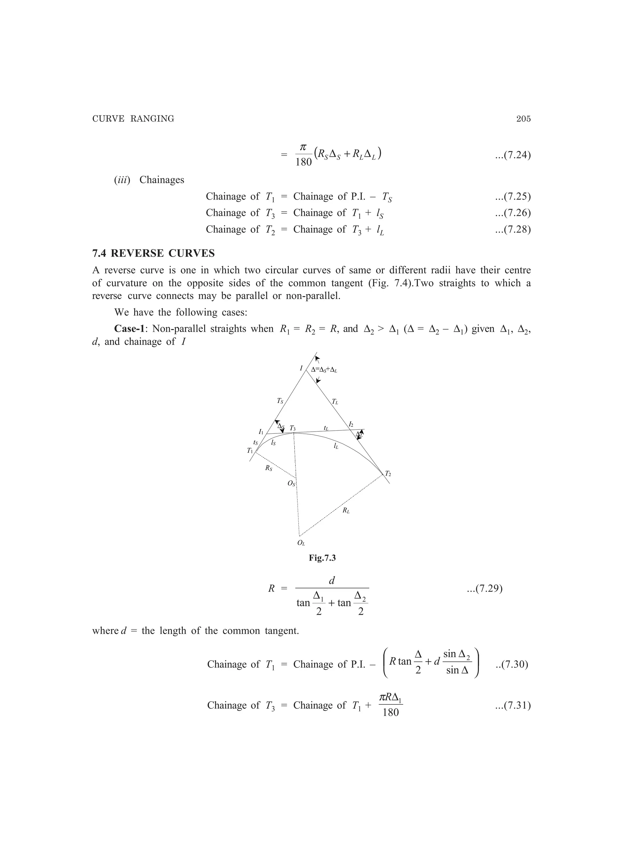
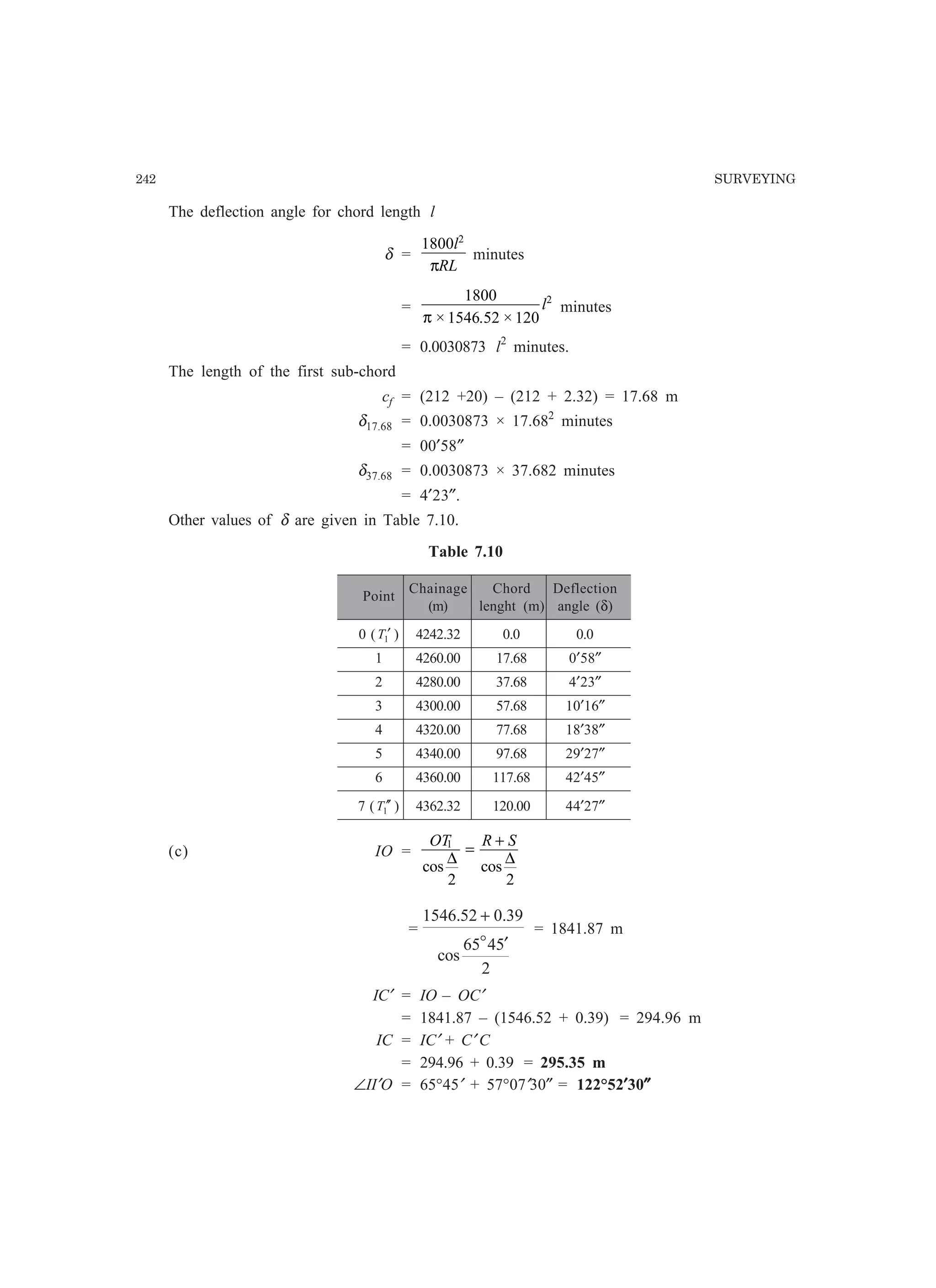
![206 SURVEYING
Chainage of T2 = Chainage of T3 +
180
2∆Rπ
...(7.32)
R1
T1
∆
O1
O2
R2
T3
T2
I1
I2
T1
T2
I
I1
I2
δ1
δ2
∆1
∆2
Fig. 7.4
Case-2: Non-parallel straights when R1 = R2 = R, given δ1, δ2, and L
R =
L
sin cos sinδ θ δ1 22+ +
...(7.33)
where θ = sin
cos cos− +F
HG I
KJ1 1 2
2
δ δ
∆1 = δ1 + (90° – θ)
∆2 = δ2 + (90° – θ).
Case-3: Non-parallel straights when R1 = R2, given δ1, δ2, L and R1 (or R2)
R2 =
−
+
−
2
sin4sin2
sin2
212
12
11
2
δδ
δ
δ
RL
LRL
...(7.35)
Case-4: Parallel straights when ∆1 = ∆2, given R1, R2,
and ∆1 (=∆2) (Fig. 7.5)
D = 2
2
1 2
2 1
R R+b gsin
∆
...(7.36)
L = ( )[ ]212 RRD + ...(7.37)
H = R R1 2 1+b gsin ∆ ...(7.38)
R1
T1
O1
O2
R2
T3
T2
H
∆1
∆2
D
Fig. 7.5](https://image.slidesharecdn.com/surveyingproblemsolving-150308103254-conversion-gate01/75/Surveying-problem-solving-219-2048.jpg)
![262 SURVEYING
Zb = (L - x) Zc +~ZD
L L
Now interpolating between a and b, in Fig. 8.5d, we get the Z coordinate of P.
f
~
tL
tL
Z - (L-x)Z 1::.ZP - ,,+ b
L L
_(L-y)[(L-X)Z Xz] y[(L-X)Z Xz]- A+- B +- c+- D
L L L L L L
= ~2 [(L -x)(L - y)ZA + x(L - y)ZB + y(L -x)Zc + XyZD]
C b D
c~.~.~.~.·· d
;~
A a B
[]J [}]
P
: z. : z i
Z, iZ. Zc iZ
' . z.cE]A~x~ BC~x~ D b
~L~ ~L~ ~L~
(b) (c) (d)
i ~--~--~--~x
O~L~L~~L~
(b) (c) (d)
(a)
(a)
Fig. 8.S
..(8.13)
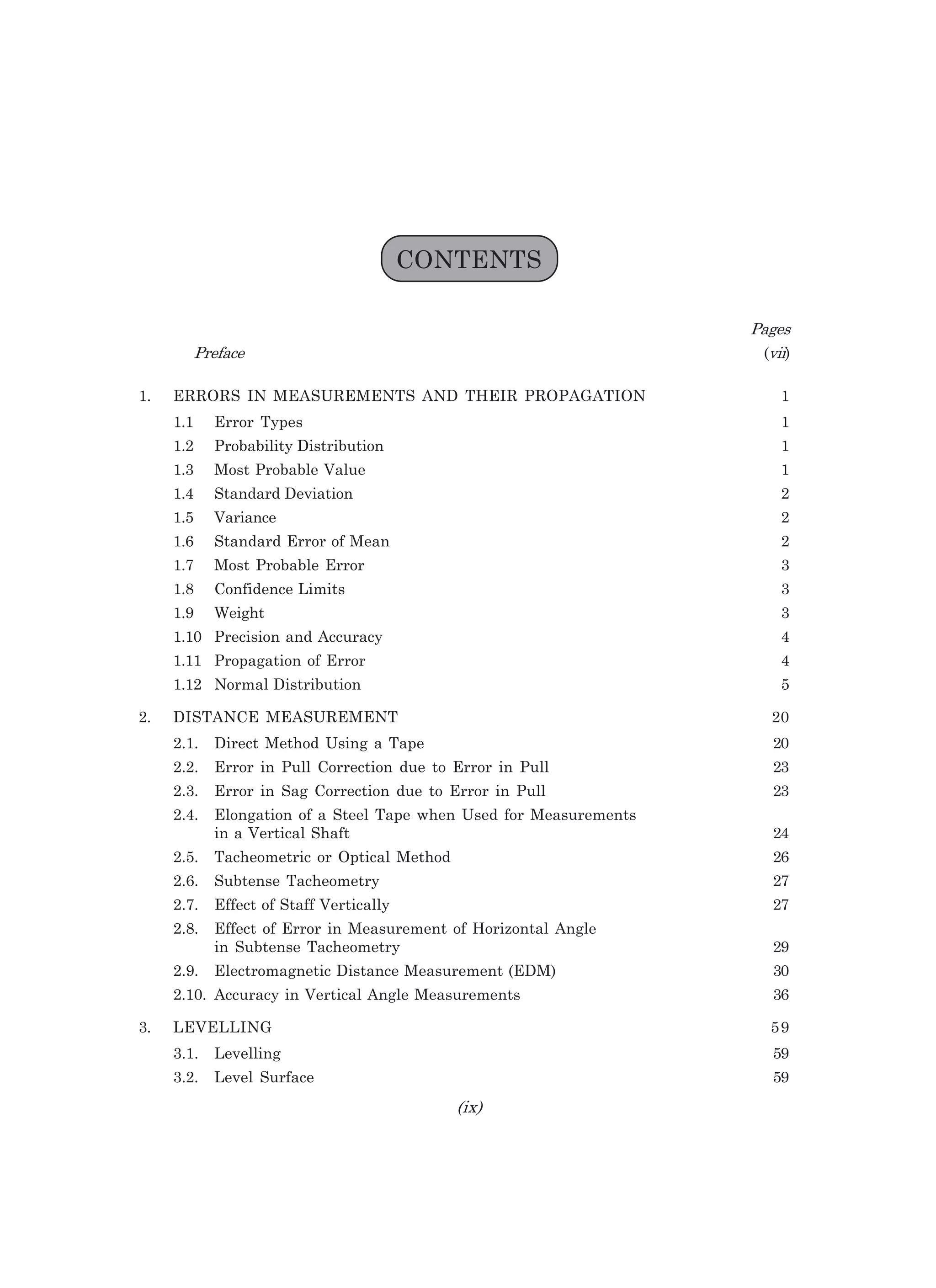
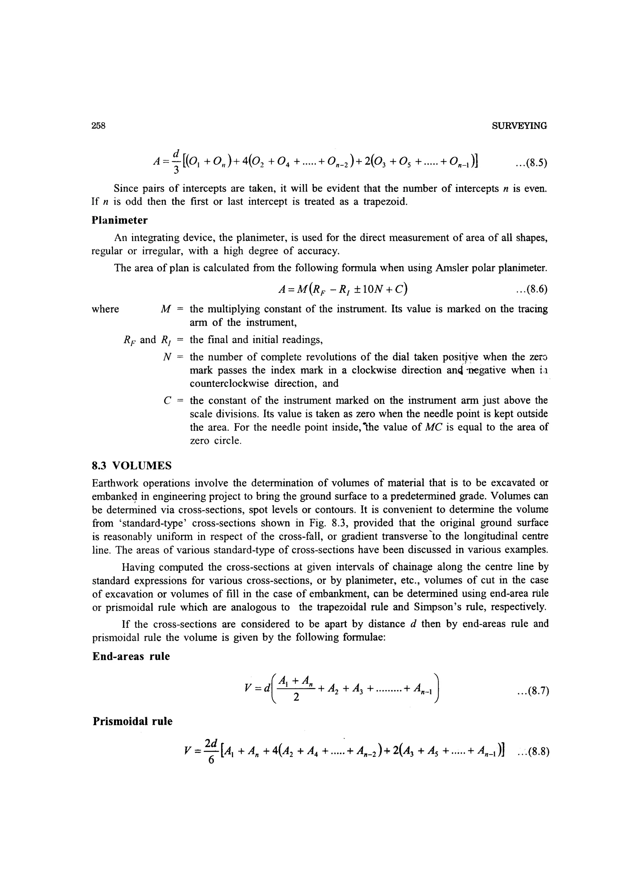
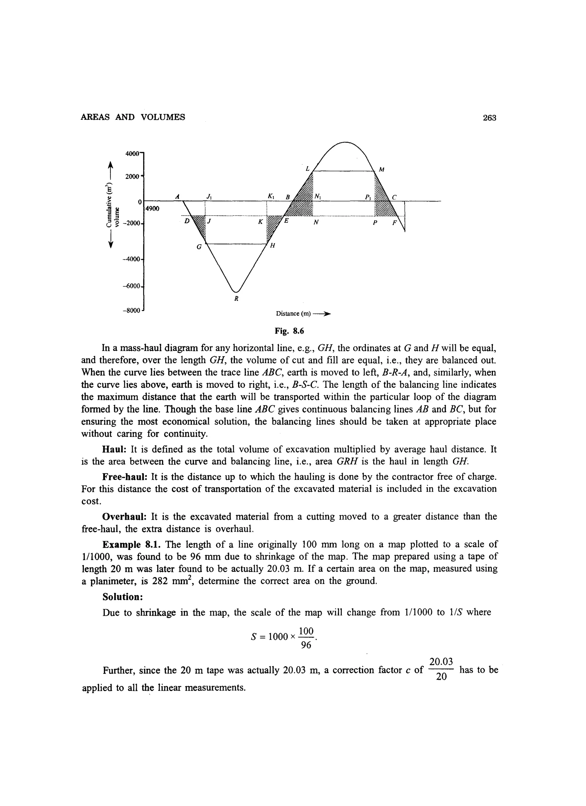
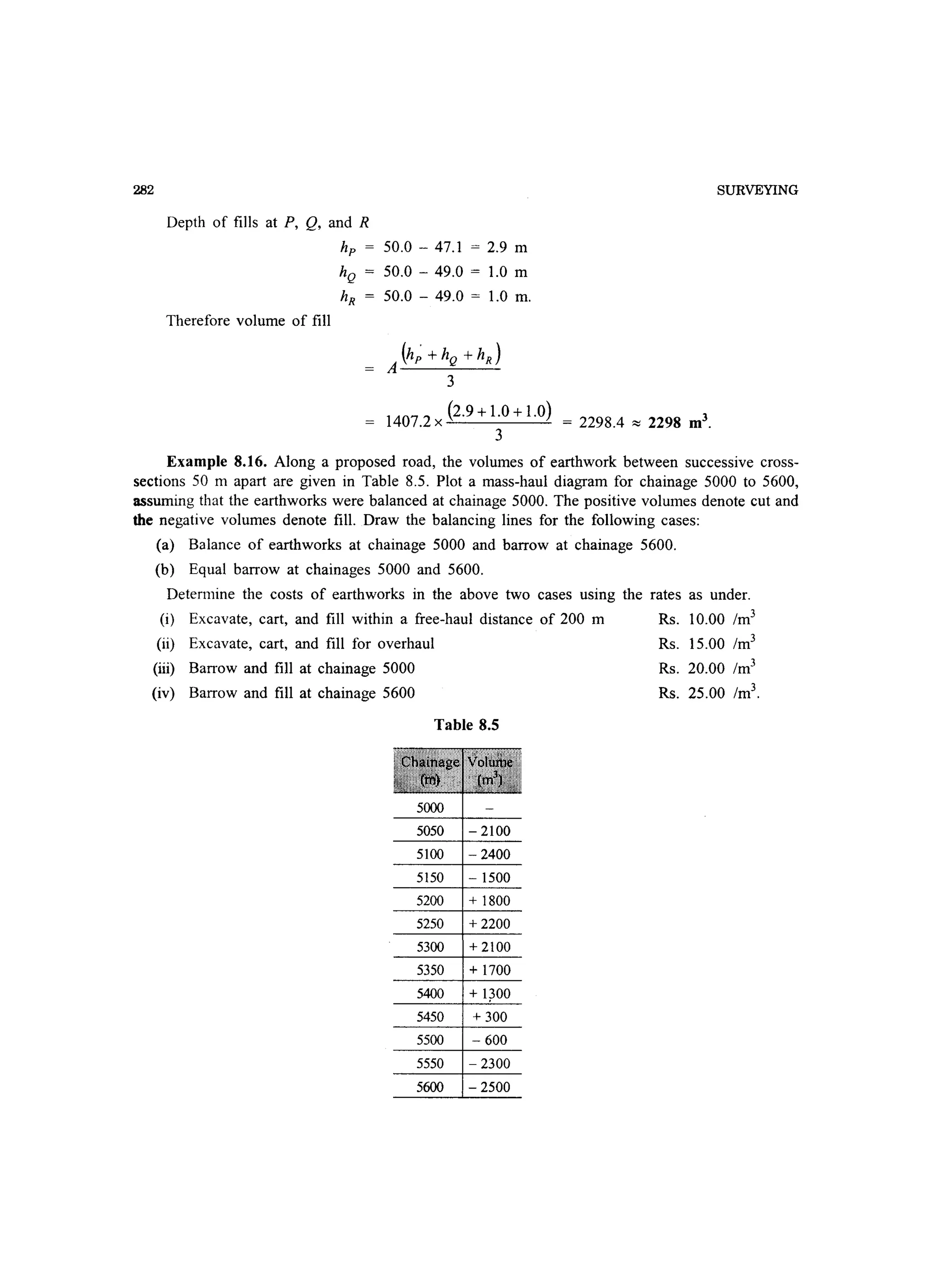
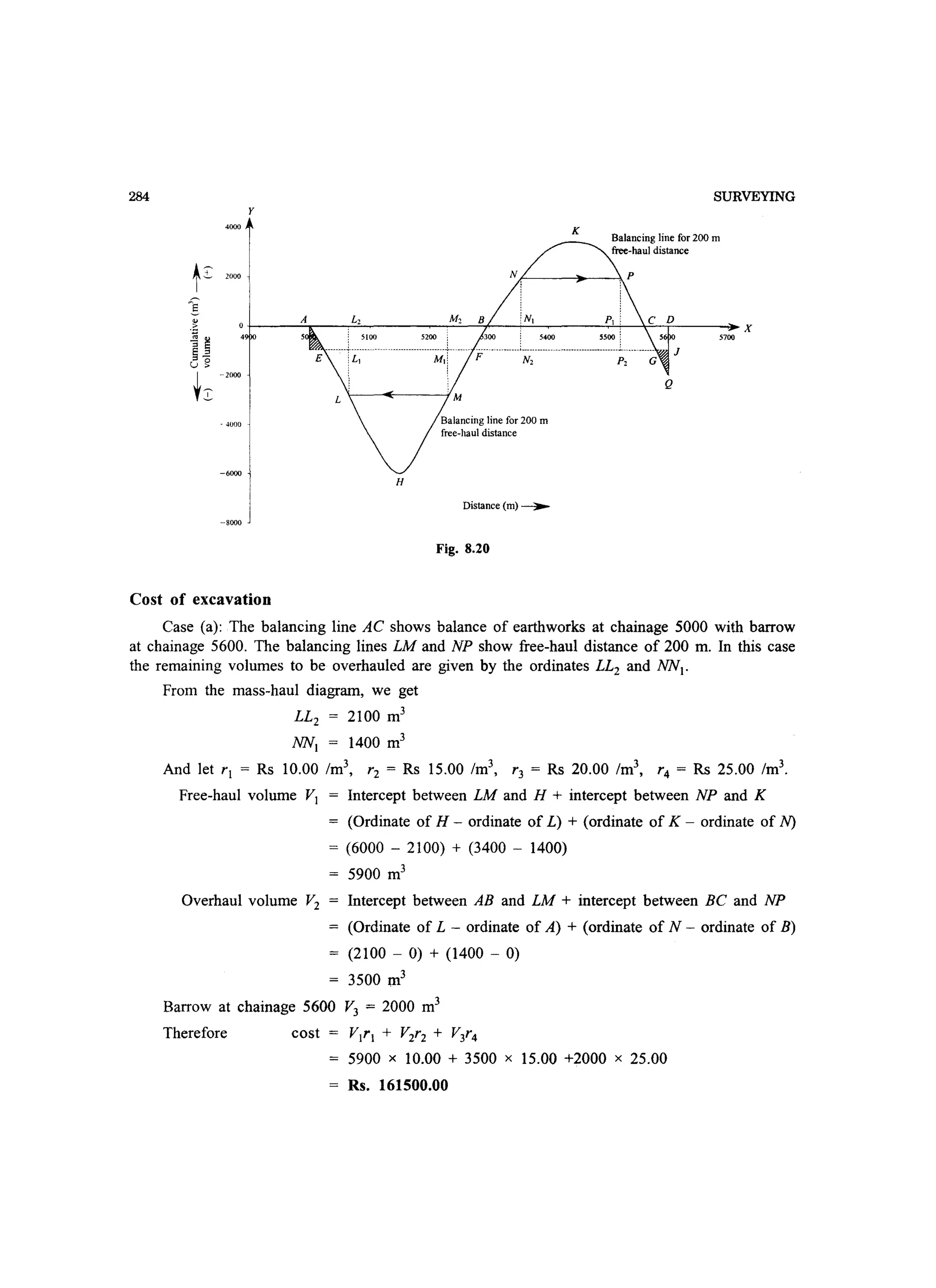
8.5 MASS-HAUL DIAGRAM
A mass-haul diagram or curve is drawn subsequent to the calculation of earthwork volumes, its
ordinates showing cumulative volumes at specific points along the centre line. Volumes of cut and
fill are treated as positive and negative, respectively. Compensation can be made as necessary, for
shrinkage or bulking of the excavated material when placed finally in an embankment.
Fig. 8.6 shows a typical mass-haul diagram in which the following characteristics of a mass-
haul diagram may be noted:
(a) A to G and S to M indicate decreasing aggregate volume which imply the formation of
embankment.
(b) Rising curve from R to B indicates a cut.
(c) R having a minimum ordinate is a point which occurs in the curve at the end of an
embankment.
(d) S having the maximum ordinate is a point which indicates the end of a cut.](https://image.slidesharecdn.com/surveyingproblemsolving-150308103254-conversion-gate01/75/Surveying-problem-solving-275-2048.jpg)
![AREAS AND VOLUMES
Thus the area
A = ~ x [0 x 320 - 0 x 170 + 170 x 90 - 320 x 470 + 470 x (-110) - 90 x 340
2
+ 340 x (- 220)- (-llO)x (- 40)+ (- 40 +} x 0 - (- 220)x 0]
= ~ x (- 296600) = - 148300 m2
2
= 148300 m2
(neglecting the sign) = 14.83 hectares.
265
It may be noted that the computed area has negative sign since the traverse has been considered
clockwise.
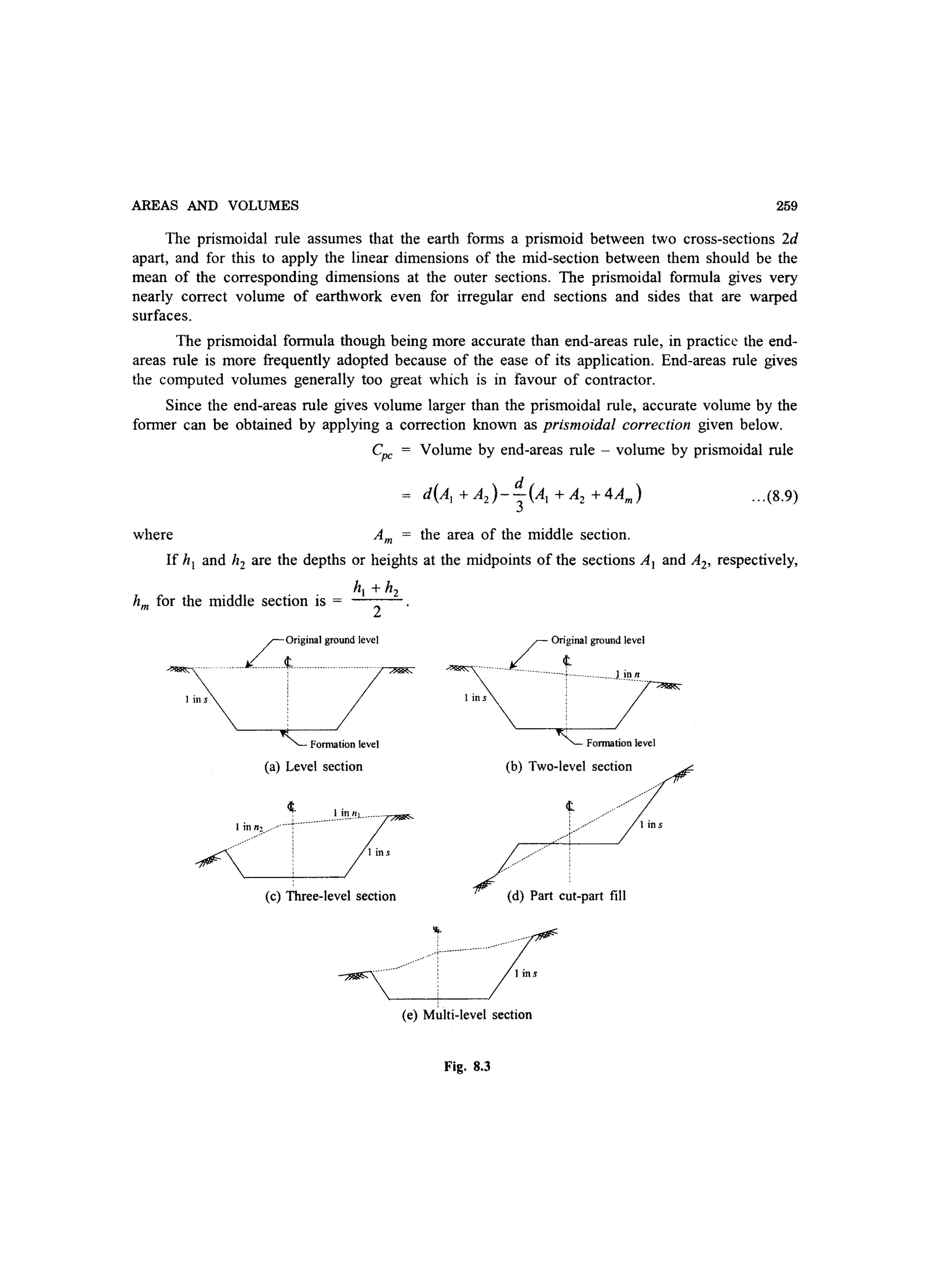
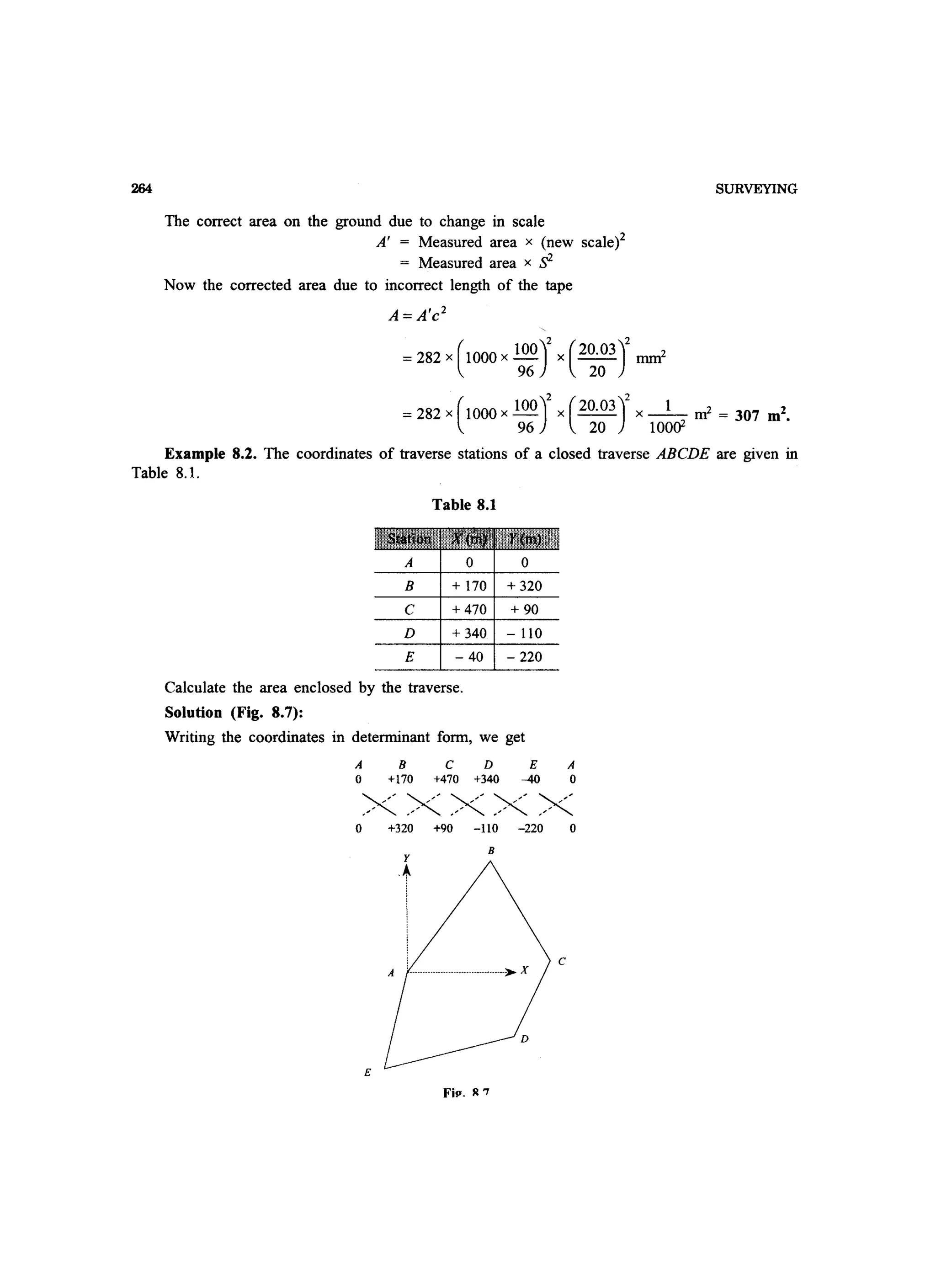
Example 8.3. A tract of land has three straight boundaries AB, BC, and CD. The fourth
boundary DA is irregular. The measured lengths are as under:
AB = 135 m, BC = 191 m, CD = 126 m, BD = 255 m.
The offsets measured outside the boundary DA to the irregular boundary at a regular interval
of 30 m from D, are as below:
0.0 30 60 90 120 150 180
0.0 3.7 4.9 4.2 2.8 3.6 0.0
Determine the area of the tract.
Solution (Fig. 8.8):
Let us first calculate the areas of triangles ABD and BCD.
The area of a triangle is given by
A = ~S(S-a)(S-b)(S-c)
S =a+b+c
in which a, b, !lnd c are the lengths of the sides, and 2
For MBD
S = 135 + 255 + 180 = 285 m
2
AI = ~285 x {285 -135}x {285 - 255}x {285 -180}... .
= 11604.42 m2
•
For MCD
S= 191+126+255 =286m
2
A2 =~286 x {286 -191}x {286 -126}x {286 - 255}
= 11608.76 m2
.
B 191 m
Fig. 8.8](https://image.slidesharecdn.com/surveyingproblemsolving-150308103254-conversion-gate01/75/Surveying-problem-solving-278-2048.jpg)
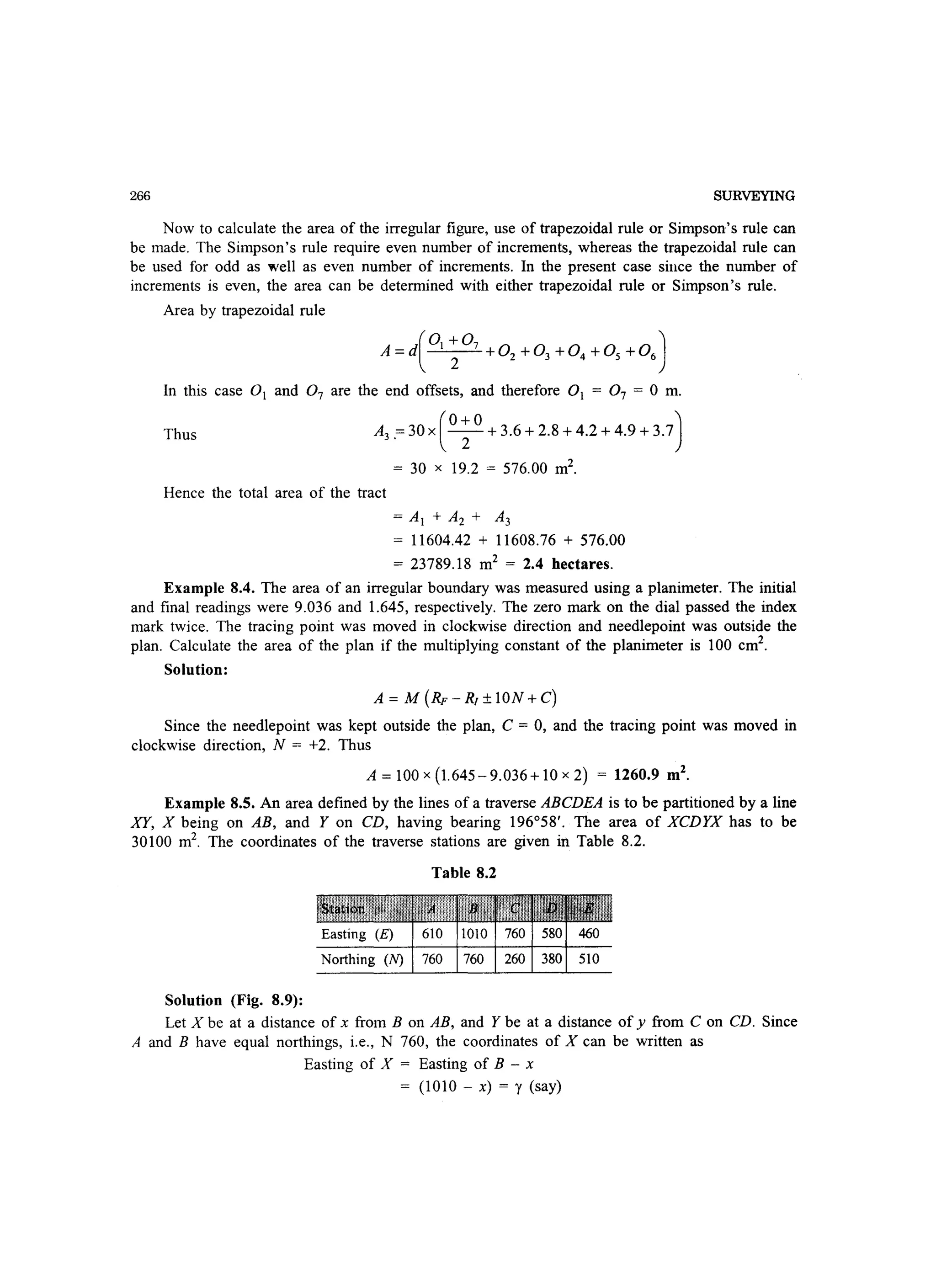
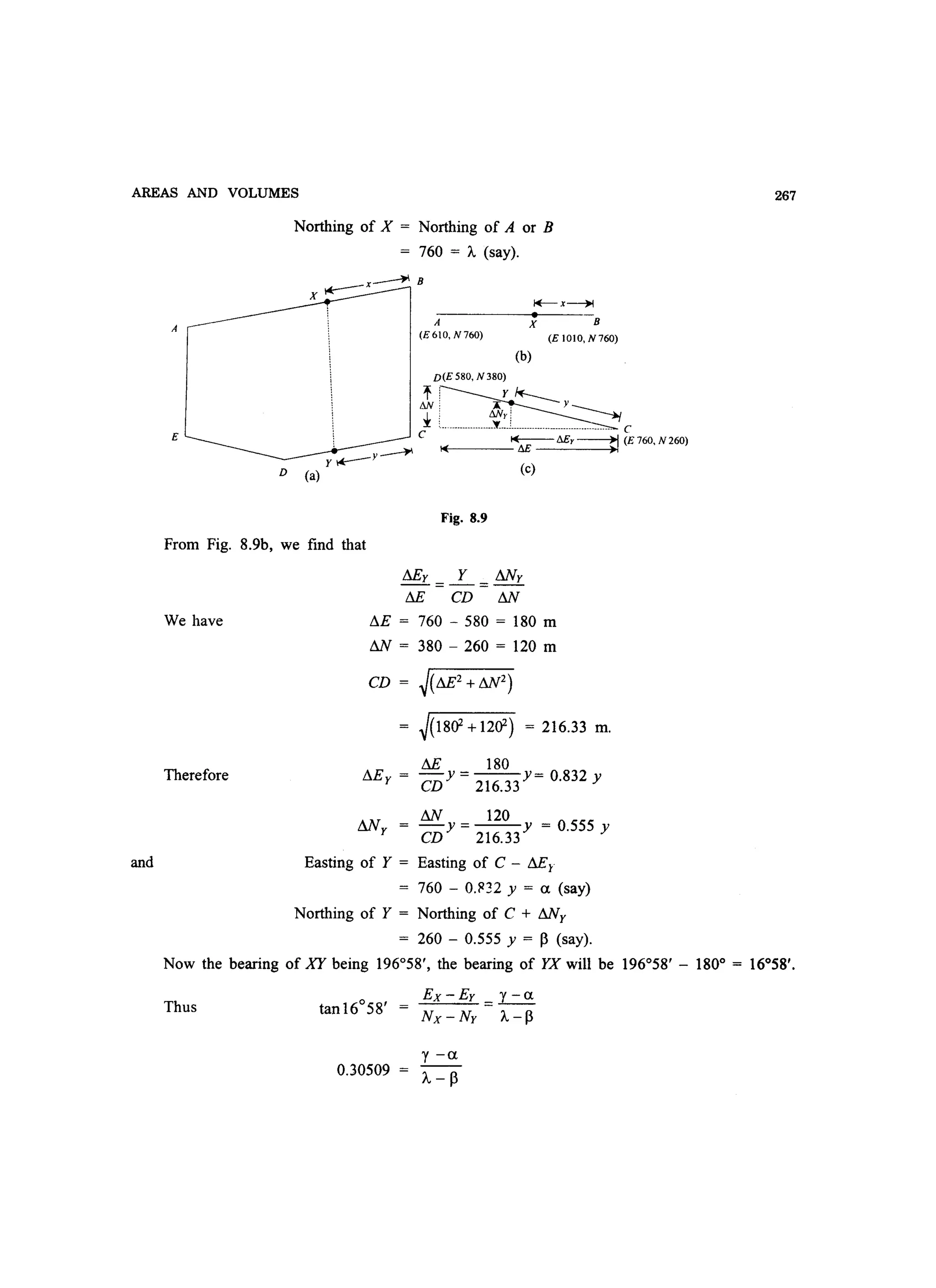
![268
y -u = 0.30509 (A - P)
1010 - x - 760 + 0.832 y = 0.30509 x (760 - 260 - 0.555 y)
x = 97.455 + 1.001 y.
Therefore Easing of X = 1010 - (97.455 + 1.001 y)
= 912.545 - 1.001 y = x' (say)
Northing of X = 760 m.
Now writing the coordinates of X, B, C, Y, and X in determinant form
X B c y x
x' 1010 760 a x'
XXXX760 760 260 760
The area of the traverse XBCYX is
SURVEYING
1
A = -x[x'x760-760x1010+1010x260-760x760+760x P-260xu
2
+ux760-pxx']
=.!.x [(760 - P)x' + 760p + 50fu -1082600]
2
1
= - x [(760 - 260 - 0.555y) x (912.545 - 1.001y) + 760 x (260 + 0.555y)
2
+ 500 x (760 - 0.832y)-1082600]
= .!.X[0.556y2 -1001.312y-48727.5]
2
Since the traverse XBCYX has been considered in clockwise direction, the sign of the computed
area will be negative. Therefore
.!.X [0.556y 2 -1001.312y - 48727.5] =- 30100
2
0.556y2 -1001.312y - 48727.5 = - 60200
0.556y2 -1001.312y + 11472.5 = 0](https://image.slidesharecdn.com/surveyingproblemsolving-150308103254-conversion-gate01/75/Surveying-problem-solving-281-2048.jpg)
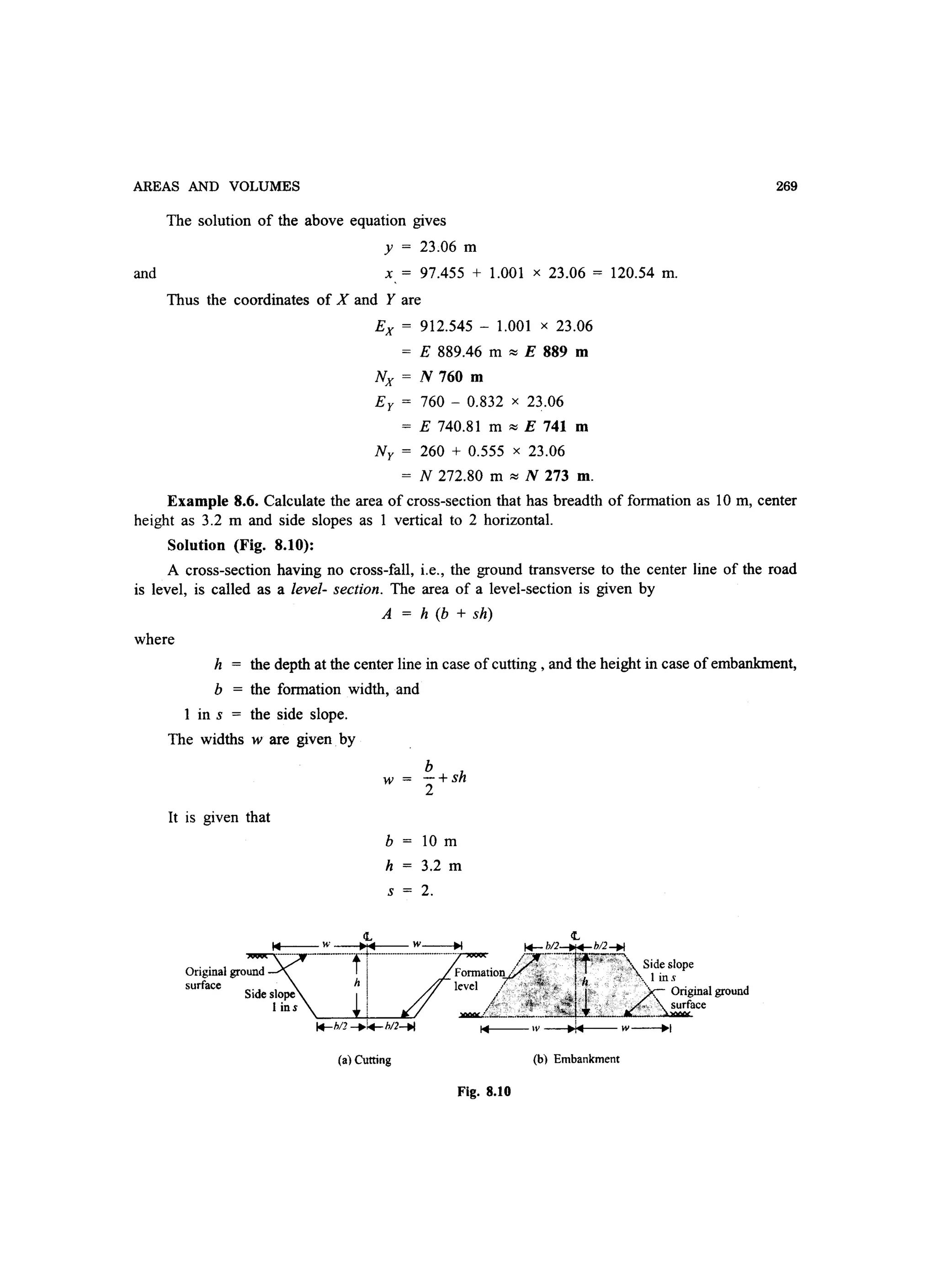
![270 SURVEYING
Hence the area
A = 3.2 x (10 + 2 x 3.2) = 52.48 m2
.
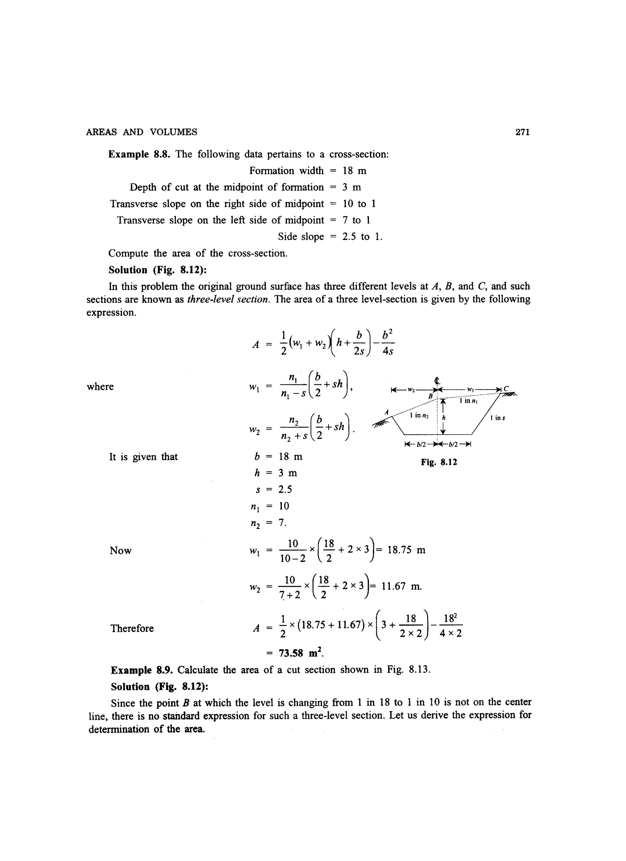
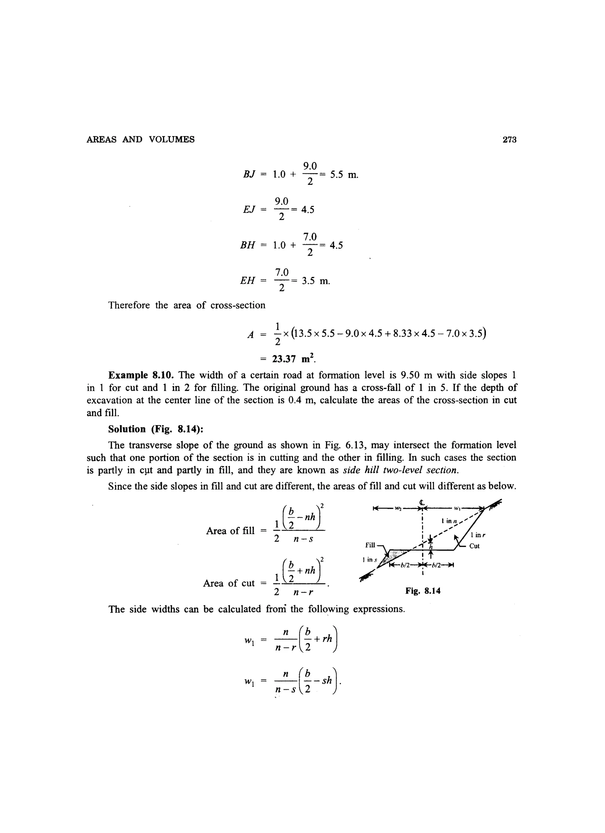
Example 8.7. Compute the area of cross-section if the formation width is 12 m, side slopes
are I to I, average height along the center line is 5 m, and the transverse slope of the ground is
10 to 1.
Solution (Fig. 8.11):
A cross-section that has a cross-fall is known as two-level section. For such sections the area
is given by
where
_n_(!.+Sh), a,1'1d
n+s 2
1 in n = the cross·-fall of the ground.
(a) Cutting (b) Embankment
Fig. 8.11
From the given data, we have
b 12 m
h 5m
s = 1
n = 10.
To calculate the area, let us first calculate wI and w2'
wI = ~X(~+lX5)= 12.22 m
10-1 2
10 (12 )w2 10+1 x 2+ 1x5 = 10.00 m.
Therefore A -.x -+lx5 (12.22+10.00)-- = 157.00 m2
.1 [(12) 122]
2xl 2 2](https://image.slidesharecdn.com/surveyingproblemsolving-150308103254-conversion-gate01/75/Surveying-problem-solving-283-2048.jpg)

![AREAS AND VOLUMES
The volume of fill is'given by the end-areas rule, i.e.,
V = d(Al ~ A3 + A2 )
and by prismoidal rule
where AI' A2, and A3 are the areas of the three cross-sections.
The following are given
b = 20 m
s = 2.5
n = 10
d = 50 m
hI' h2' h3 = 3.3 m, 4.1 m, 4.9 m.
For section-l
_1_0_x (_20 + 2.5 x 3.3J= 2427 m
10- 2.5 2 .
_1_0_ x (_20 + 2.5 x 3.3J = 14.60 m
10+2.5 2
1 x [(20 + 2.5 x 3.3J x (24.27 + 14.60)- 20
2
]
2x 2.5 2 2
101.88 m2
.
For section-2
10 x(20 +2.5X4.1J = 26.93 m
10-2.5 2
_1_0_X(_20 +2.5X4.1J = 16.20 m
10+ 2.5 2
1 x[(20 + 2.5 X4.1J x (26.93 +16.20)- 20
2
]
2x 2.5 2 2
134.68 m2
.
For section-3
_1_0_x (_20 + 2.5 x 4.9J = 29.59 m
10- 2.5 2
275](https://image.slidesharecdn.com/surveyingproblemsolving-150308103254-conversion-gate01/75/Surveying-problem-solving-288-2048.jpg)
![276
Therefore
by end-areas rule
and by prismoidal rule
SURVEYING
Wz _1_0_X(_20 +2.5 X4.9)= 17.80 m
10+ 2.5 2
1 x [(20 + 2.5 x 4.9) x (29.59 + 17.80)- 20
2
]
2x 2.5 2 2
170.89 mZ
•
v = 50 x C°1.88; 170.89 + 134.68)
13553.3 ~ 13553 m3
.
v = 50 x (101.88 + 170.89 + 4 x 134.68)
3
13524.8 ~ 13525 m3
.
Since the end-areas rule gives the higher value of volume than the prismoidal rule, the volume
by the former can be corrected by applying prismoidal correction given by the following formula
for a two-level section.
Cpc
50 (102
J- x 2.5 x 2 2 = 22.22
6 10 - 2.5
Now 22.22x(3.3-4.1Y= 14.22 m3
Total correction
Cpc = Cpcl + Cpcz = 2 x 14.22 = 28.44 m3
.
Thus the corrected end-areas volume
= 13553 - 28.44 = 13524.56 ~ 13525 m3
.
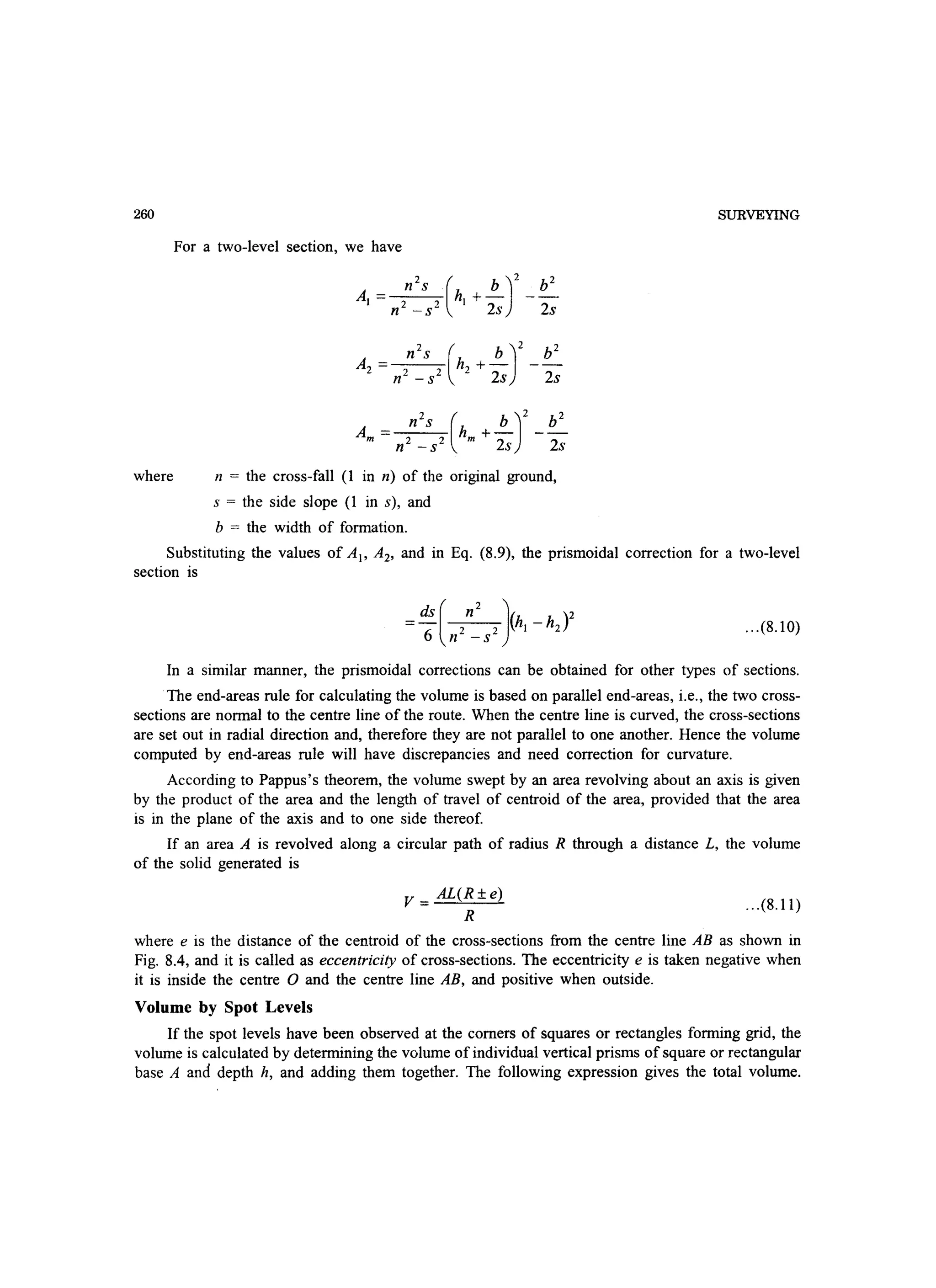
Example 8.12. Fig. 8.15 shows the distribution of 12 spot heights with a regular 20 m spacing
covering a rectangular area which is to be graded to form a horizontal plane having an elevation
of 10.00 m. Calculate the volume of the earth.
Solution (Fig. 8.15):
Since the finished horizontal surface has the elevation of 10.00 m, the heights of the comers
above the finished surface will be (h - 10.00) where h is the spot heights of the points.](https://image.slidesharecdn.com/surveyingproblemsolving-150308103254-conversion-gate01/75/Surveying-problem-solving-289-2048.jpg)
![AREAS AND VOLUMES
Now
[.h! 17.18 + 17.76 + 18.38 + 17.76 = 71.08 m
[.h2 17.52 + 18.00 + 18.29 + 18.24 + 17.63 + 17.32 = 107.00 m
[.h3
0
[.h4 17.69 + 18.11 = 35.80 m
A = 20 x 20 = 400 m2
.
The volume is given by
v = A(i./4 + 2i.~ + 3[.ft., + 4[.14)
4
i27]76
~28.00_
20
fI 27.69
20
127]18 27.32
277
~9 2~38
I
I
I
I
i
28
1
11 2sh
,
I
27.63 27176
400 x (17.08 + 2 x 107.00 + 3 x 0 + 4 x 35.80)
4
1+--20 )I( 20~~20~
Fig. 8.15
37428.00 m3
.
Example 8.13. The area having spot heights given in Example 8.12 to be graded to form a
horizontal plane at a level where cut and fill are balanced. Assuming no bulking or shrinking of the
excavated earth and neglecting any effects of side slopes, determine the design level.
Solution (Fig. 8.15):
Let the design level be h. Thus
[.h! (27.18 - h) + (27.76 - h) + (28.38 - h) + (27.76 - h) = 111.08 - 4h
[.h2 (27.52 - h) + (28.00 - h) + (28.29 - h) + (28.24 - h) + (27.63 - h) + (27.32 - h)
167.00 - 6h
[.h3 0
[.h4 (27.69 - h) + (28.11 - h) = 55.80 - 2h.
Since the cut and fill are balanced, there will be no residual volume of excavated earth,
therefore
v = 4~0 x[(111.08-4h)+2(167.00-6h)+3xO+4(55.80-2h)]
o 668.28 - 24h
668.28
h =
24
= 27.85 m.
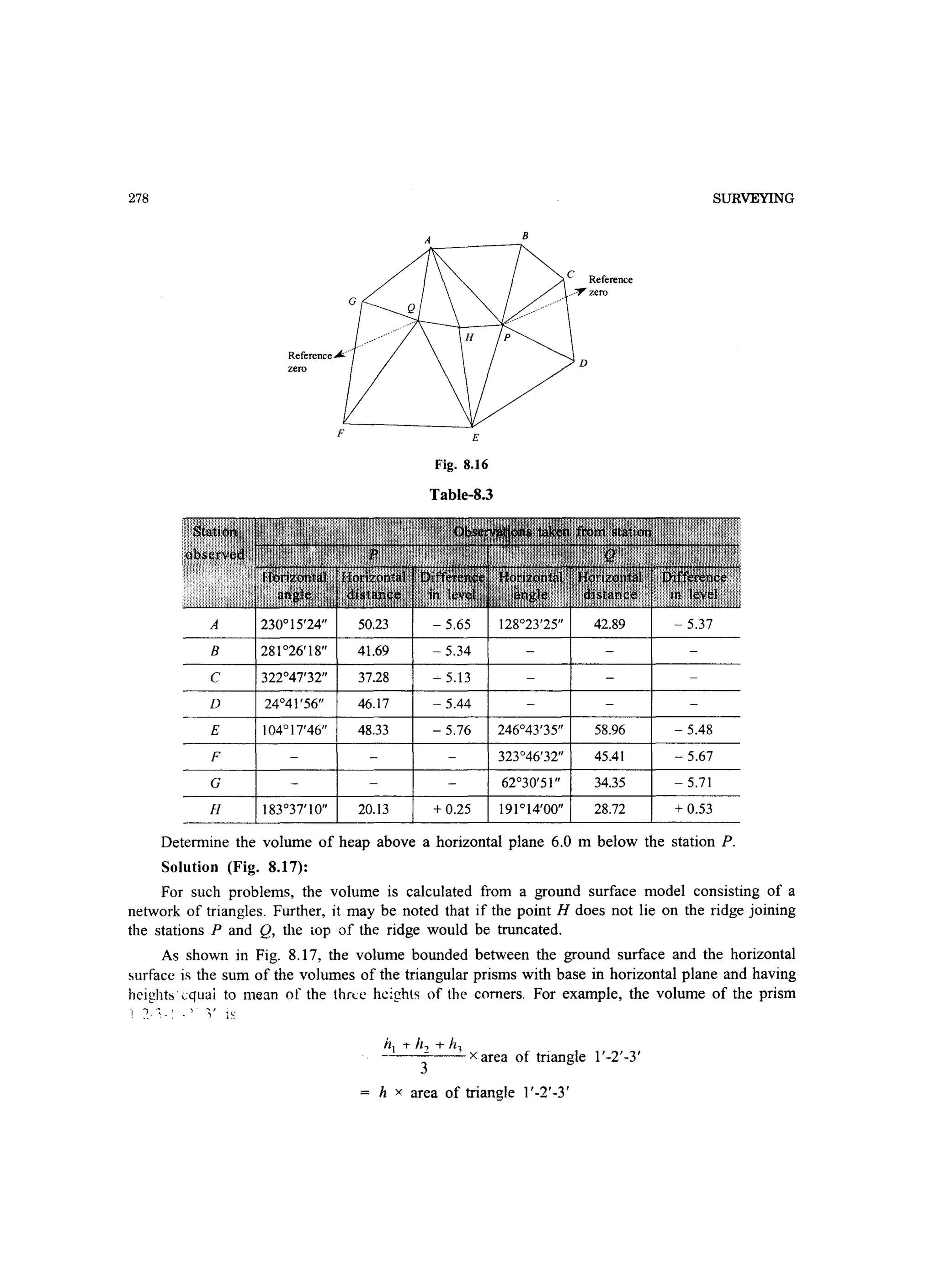
Example 8.14. The stations P and Q were established on the top of a spoil heap as shown
in Fig. 8.16. Seven points were established at the base of the heap and one at the top on the line
PQ. The observations given in Table 8.3 were recorded using a total station instrument from the.
stations P and Q keeping the heights of instrument and prism equal at both the stations.](https://image.slidesharecdn.com/surveyingproblemsolving-150308103254-conversion-gate01/75/Surveying-problem-solving-290-2048.jpg)
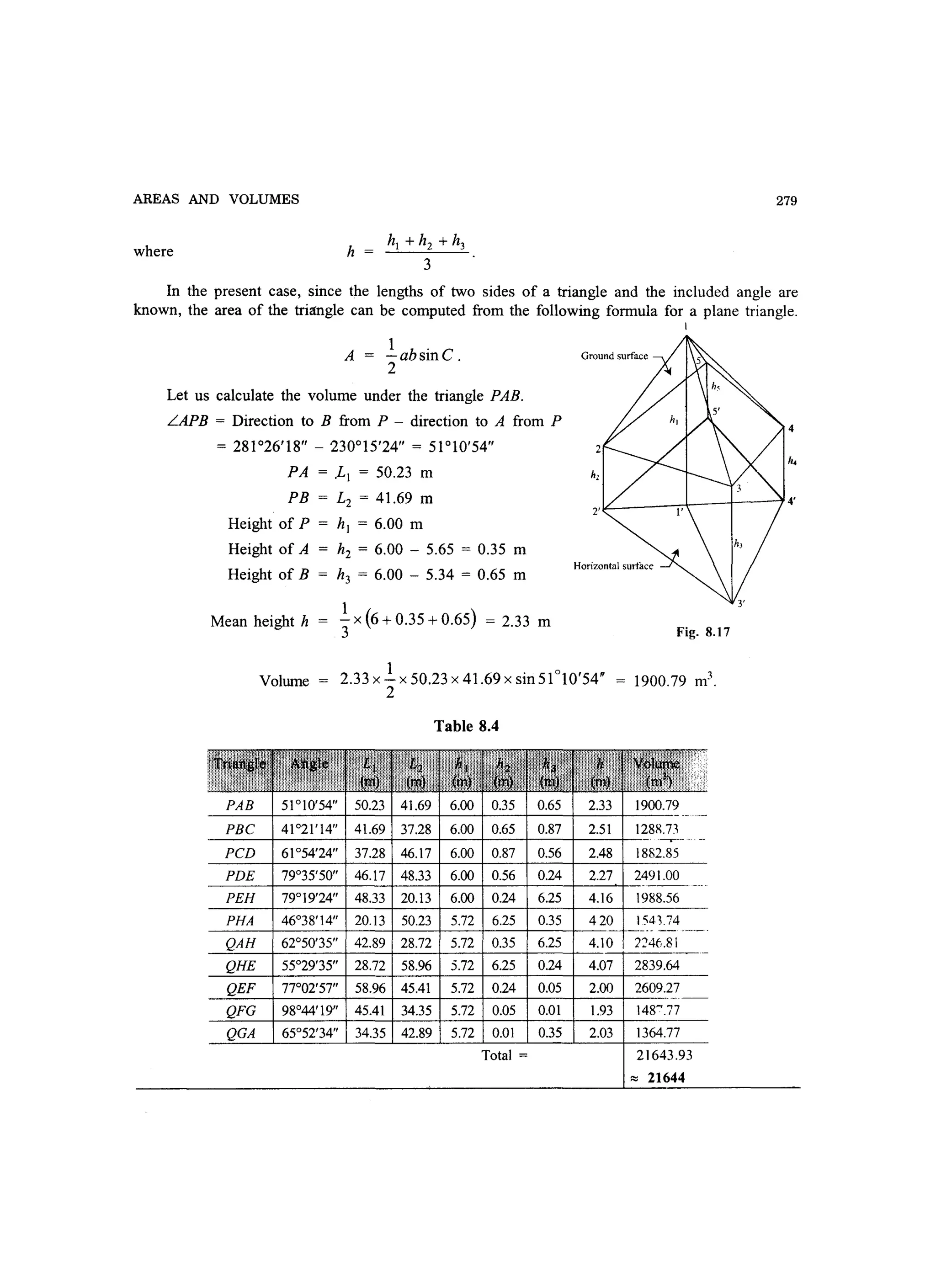
![280 SURVEYING
The horizontal plane is 6 m below P, or (6 + 0.25) = 6.25 m below H, or (6.25 - 0.53) =
5.72 m below Q. Therefore, to calculate the heights of the comers of the triangles, observed from
P, the height 6.00 m of P, and observed from Q, the height 5.72 m of Q, above the horizontal plane
have to be considered.
Table 8.4 gives the necessary data to calculate the volume of triangular prisms.
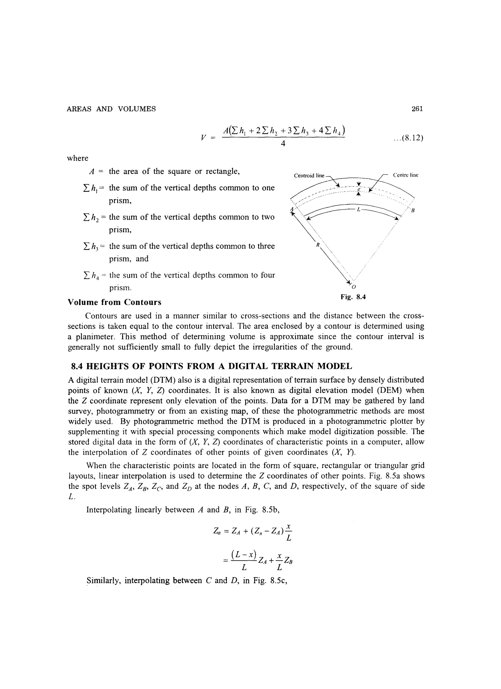
Example 8.15. Fig. 8.18 shows the spot heights at the nodes of the squares of 20 m side in
certain area. With origin at 0, three points P, Q, and R were located having coordinates as
(23.0 m, 44.0 m), (86.0 m, 48.0 m), and (65.0 m, 2.0 m), respectively. It is proposed to raise the
area PQR to a level of 50.00 m above datum. Determine the volume of earthwork required to fill
the area.
i'-'i.~ .'- H'-:' ~ -
46~5 _ _A6j-__A7.5 _ 4lLl __48.7_~_Q'
I ;-pr~~~:----------------------r}:
46,5 4710_' '4.7.7 _48.4_ 49.0 -I ._
, ~, /
! 'I ' ' /
411--- 41..4___ .48.Q -4,~6.-__ 4~
i i , R!
47[4____ 47..9 __ 48.5- 48:'r~~~'I{49l3-
o
Fig. 8.18
Solution (Fig. 8.18):
46.8 47_5
Fig. 8.19
To determine the heights of the points P, Q, and R above datum, let us define the squares as
shown in Fig. 8.19.
For the point P
L
x
L-x
y
L - Y
20
23.0 - 20 = 3.0 m
20 - 3.0 = 17.0 m
44.0 - 40 = 4.0 m
20 - 4.0 = 16.0 m
ZA 47.0 m, ZB = 47.7 m, Zc = 46.8 m, ZD = 47.5 m.
Zp
1
-x [17.0 xI6.0x47.0 +3.0xI6.0x47.7 +4.0xI7.0x46.8
202
+3.0 x 4.0x 47.5]
47.1 m.](https://image.slidesharecdn.com/surveyingproblemsolving-150308103254-conversion-gate01/75/Surveying-problem-solving-293-2048.jpg)
![AREAS AND VOLUMES
For th~ point Q
For the point R
The area of !:lPQR
x = 86.0 - 80 = 6.0 m
L - x = 20 - 6.0 = 14.0 m
y = 48.0 - 40 = 8.0 m
L - y = 20 - 8.0 = 12.0 m
ZA = 49.0 m, ZB = 49.3 m, Zc = 48.7 m, ZD = 48.9 m.
281
1
ZQ = -2 X [14.0 x 12.0 x 49.0 + 6.0 x 12.0 x 49.3 + 8.0 x 14.0 x 48.7
20
-+ 6.0 x 8.0 x 48.9]
= 49.0 m.
x = 65.0 - 60 = 5.0 m
L - x = 20 - 5.0 = 15.0 m
y = 2.0 - 0 = 2.0 m
L - y = 20 - 2.0 = 18.0 m
ZA = 48.9 m, ZB = 49.3 m, Zc = 48.6 m, ZD = 49.0 m.
1
ZR = -2 x [15.0 x 18.0 x 48.9 + 5.0 x 18.0 x 49.3 + 2.0 x 15.0 x 48.6
20
+ 5.0 x 2.0 x 49.0]
= 49.0 m.
PQ = ~(23.0-86.0)2 +(44.0-48.0)2 = 63.13 m
QR = ~(86.0-65.0)2+(48.0-2.0)2 = 50.57 m
RP = ~(65.0-23.of +(2.0-44.0)2 = 59.40 m
S = l.(PQ+QR+RP)
2
.!.x(63.13+50.57+59.40) = 86.55 m.
2
Area A = ~[S(S - PQ){S - QR)(S - RP)]
~86.55 x {86.55 - 63.13}x {86.55 - 50.57}x {86.55 - 59.40}
1407.2 m2
.](https://image.slidesharecdn.com/surveyingproblemsolving-150308103254-conversion-gate01/75/Surveying-problem-solving-294-2048.jpg)
![290 SURVEYING
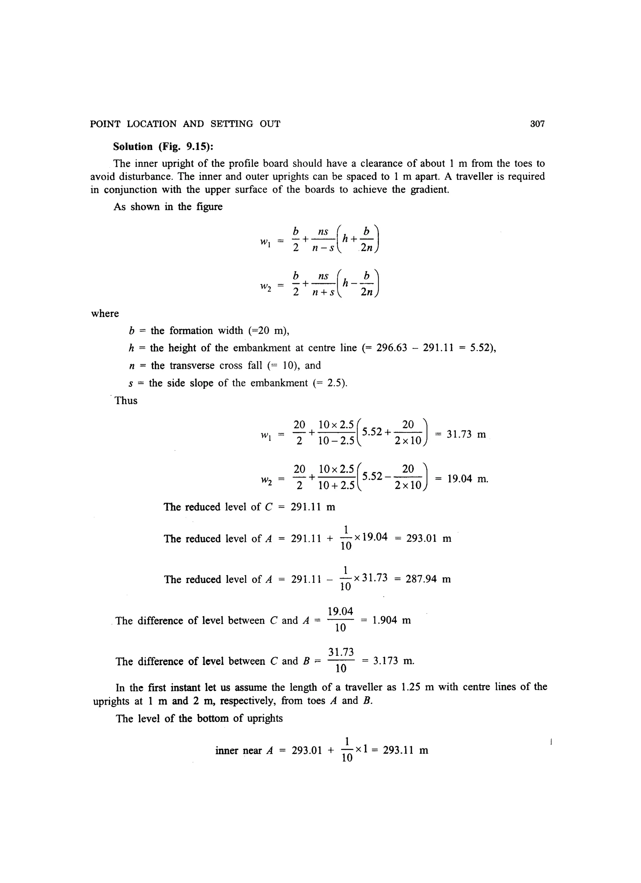
9.9 EMBANKMENT PROFILE BOARDS
The profile boards are nailed to two uprights which are firmly driven into the ground near the toes
of the embankment (Fig. 9.5). The inner uprights must have clearances from the toes of the order
of 1.0 m to prevent disturbance. The inner and outer uprights can be spaced up to 1.0 m apart,
since the sloping boards reflecting the side gradients, need to be of reasonable length for sighting
purposes. A traveller is used in conjunction with the upper surface of the boards to achieve the
gradients.
Embankment
rl1 in s Profile board
Outer upright
Fig.9.S
Example 9.1. The four comers A, B, C, and D of a rectangular building having the coordinates
given in Table 9.1, are to be set out from control station P by a total station instrument. Calculate
the WCB and distance to establish each comer of the building.
Table 9.1
A 117.984 92.849
B 82.629 128.204
c 33.132 78.707
D 68.487 43.352
The coordinates of Pare E 110.383 m, N 81.334 m.
Solution (Fig. 9.6):
For comer A
WCB of PA = epA
tan = tan ---_1[117.984 -110.383] -I[ 7.601 ]
92.849-81.334 11.515](https://image.slidesharecdn.com/surveyingproblemsolving-150308103254-conversion-gate01/75/Surveying-problem-solving-303-2048.jpg)
![POINT LOCATION AND SETTING OUT
For comer B
weB of PB = aPB
PA = ~(EA -Ep)2 +(NA-Np)2
.J7.6012
+11.5152
13.797 m.
_1[82.629 -110.383]tan
128.204 - 81.334
_1[-27.754]= tan
46.870
= 30°37'55 (from a calculator)
291
Fig. 9.6
The whole circle bearings are never negative. The computed value using a calculator is from
trigonometric functions relative to north-south axis with positive and negative signs depending upon
the quadrant containing the angle. The tangent value of an angle is positive or negative as shown
in Fig. 9.7.
In this case northing of B is greater than that of P so B must lie in the fourth quadrant.
Therefore
apB
PB
For comer C
WeB of PC =
360° - 30°37'55 = 329°22'05
~(-27.754)2 +46.8702
a - t -l[ Ee - Ep ]PC - an
Ne-Np
tan-l[ 33.132 -110.383]
78.707 - 81.334
tan-1[-77.251 ]
-2.627
= 54.471
c········
West I
88°03'08 (from a calculator)
c•••
m.
IV
- Departure
+ Latitude
tan = - value
III
-Departure
- Latitude
tan = + value
North
........
~
South
Fig. 9.7
+ Departure
+ Latitude
tan = + value
II
+ Departure
- Latitude
tan = - value
East
......
Since both easting and northing of C are less that those of P as indicated by the negative signs
in numerator and denominator of the calculation of tan-I, the point C must be in the third quadrant
to get the positive value of the tangent of WeB. Therefore](https://image.slidesharecdn.com/surveyingproblemsolving-150308103254-conversion-gate01/75/Surveying-problem-solving-304-2048.jpg)
![292
For corner D
apc = 180° + 88°03'08 = 268°03'08
PC = ~(-77.251Y +(- 2.627Y = 77.296 m.
WCB of PD = apD
_1[68.487 -110.383]tan
43.352 - 81.334
SURVEYING
_1[-41.896]
= tan = 47°48'19 (from a calculator)
-37.982
The point D is also in the third quadrant due to the same reasons as for C above. Therefore
aPD = 180° + 47°48'19 = 227°48'192
PD = ~(-41.896)2 +(-37.982Y = 56.55 m.
Example 9.2. From two triangulation stations A and B the clockwise horizontal angles to a
station C were measured as LBAC = 50°05'262
and LABC = 321°55'442
• Determine the coordinates
of C given those of A and Bare
A E 1000.00 m N 1350.00 m
B E 1133.50 m N 1450.00 m.
Solution (Fig. 9.8):
a 50°05'26
P 360° - 321°55'442
= 38°04'16.
If the coordinates of A, B, and Care (EA' NA), (EB' NB), and (Eo Nd, respectively, then
BD = EB - EA 1133.50 - 1000.00 = 133.50 m
AD = NB - NA
Therefore bearing of AB
1450.00 - 1350.00 = 100.00 m.
a tan-I BD.
AD
_1133.50
tan = 53°09'52.
100.0
Bearing of AC = aAC = Bearing of AB + a
53°09'52 + 50°05'26
D:----
0..._.
A
--c
Fig. 9.8](https://image.slidesharecdn.com/surveyingproblemsolving-150308103254-conversion-gate01/75/Surveying-problem-solving-305-2048.jpg)
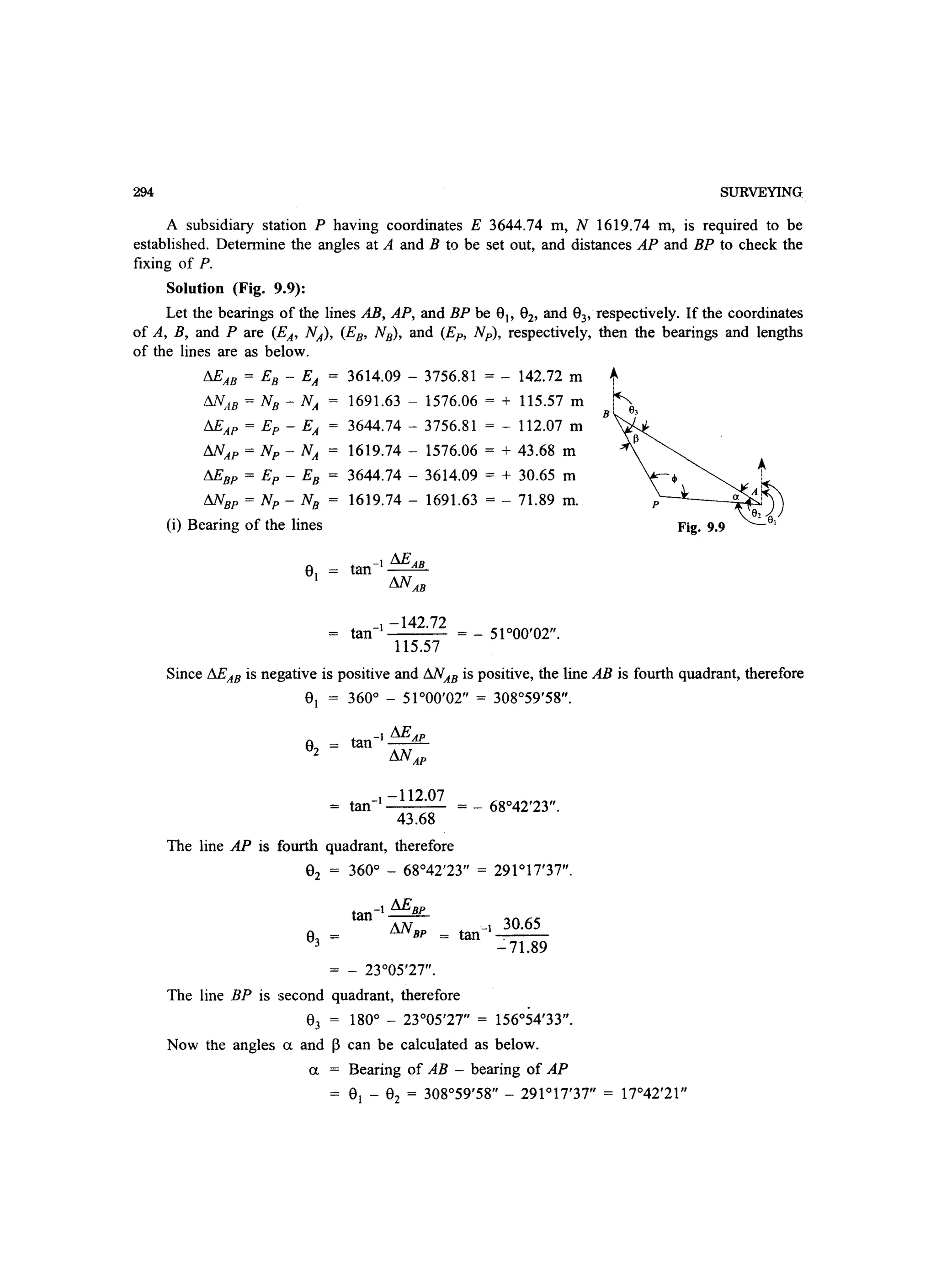
![POINT LOCATION AND SETTING OUT 295
P = Bearing of BP - back bearing of AB
= 8, - 82 = 156°54'33 - (180° + 308°59'582
- 360°) = 27°54'352•
To check the computations
I = (360° - back bearing of BP) + back bearing of AP
= [360° - (180° - 156°54'332
)] + (180° + 291°17'372
) = 134°23'042
Now, in !:!.APB we should have
a + P+ I
17°42'21 + 27°54'35 + f34°23'04 180° (Okay).
Lengths of the lines
Thus
~(-112.07r + 43.68 2
= 120.28 m.
~30.652 +(-71.89)2 = 78.15 m.
LBAP = 17°42'21
LABP = 27°54'35
AP = 120.28 m
BP = 78.15 m.
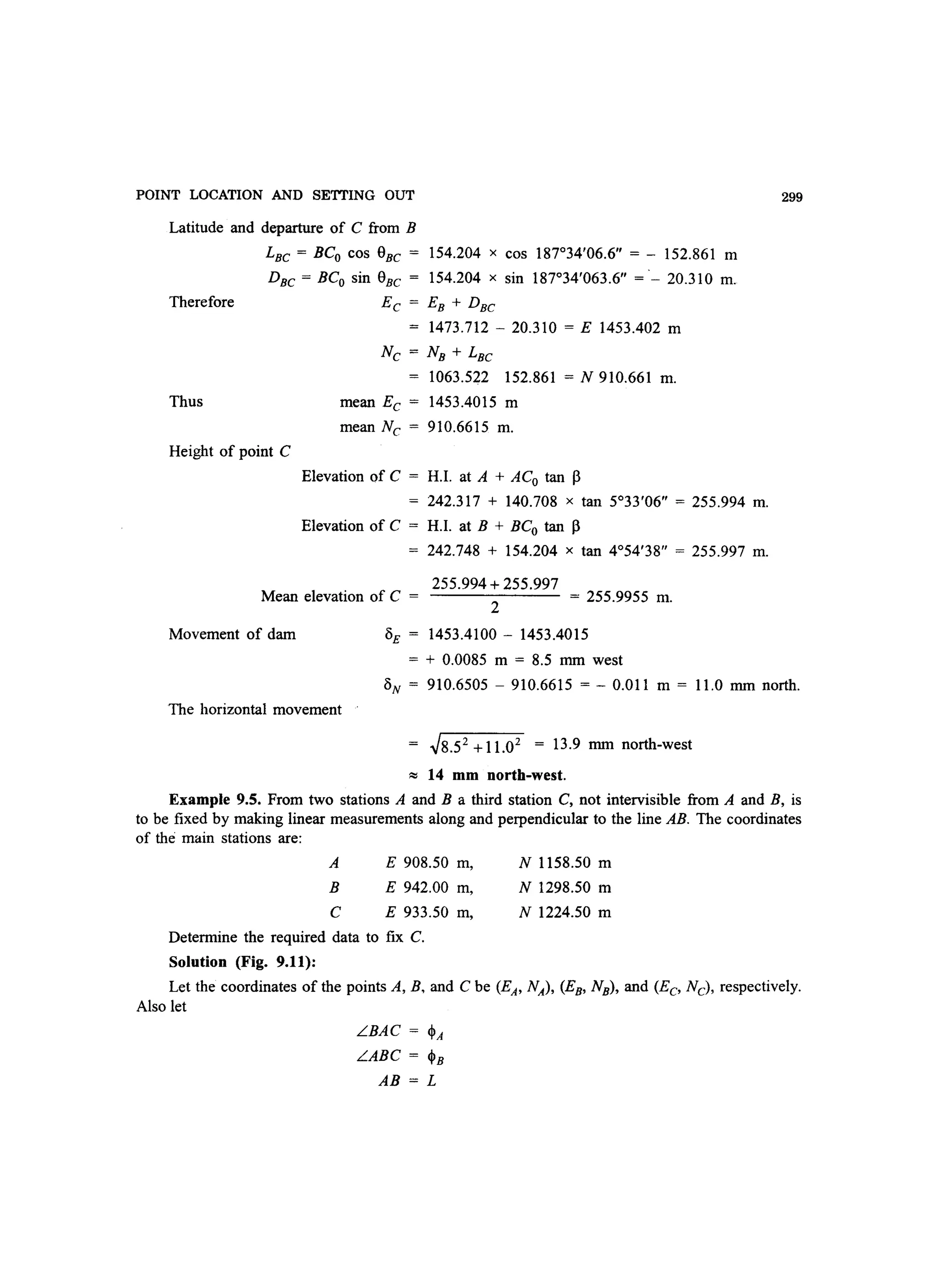
Example 9.4. To monitor the movement of dam, the observations were made on a target C
attached to the wall of the dam from two fixed concrete pillars A and B, situated to the north-west
of the dam. The coordinates and elevations of the pillar tops on which a theodolite can be mounted
for making observations, are:
A E 1322.281 m, N 961.713 m, 241.831 m
B E 1473.712 m N 1063.522 m, 242.262 m
The observations given in Table-9.2, were made with a theodolite having the height of collimation
486 m above the pillar top. If the height of C is given by the mean observations from A and B,
determine its movement after the reservoir is filled.
Solution (Fig. 9.10):
The given data are
Table 9.2
B Horizontal LABC 48°31' 18 48°31 '05
Vertical angle LC +4°54'42 +4°54'38
EA. NA = E 1322.281 m, N 961.713 m
EB, NB = E 1473.712 m, N 1063.522'm](https://image.slidesharecdn.com/surveyingproblemsolving-150308103254-conversion-gate01/75/Surveying-problem-solving-308-2048.jpg)
![296
hA = 241.831 m
hB = 242.262 m
hi = 486 mm
eA LBAC
eB LABC
ex Vertical angle to C at A
13 = Vertical angle to C at B.
Fig. 9.10
Bearing 4 of AB = tan-1[EB - EA ]
NB -NA
The line AB is in first quadrant, therefore
_1[1473.712 -1322.281J
tan
1063.522 - 961.713
tan-1[151.431J = 56005'11.6.
101.809
4 56°05'11.6.
AB ~(EB -EJ2 +(NB -NJ2
SURVEYING
= ~151.4312 +101.8092 = 182.473 m.](https://image.slidesharecdn.com/surveyingproblemsolving-150308103254-conversion-gate01/75/Surveying-problem-solving-309-2048.jpg)
![302
Solution (Fig. 9.12):
From the given data, we get
AB = ~(EA -EB)2 +(NA-NBY
~(1550-1500Y+(1600 -1450Y
= ~502 +1502 = 158.114 m.
-I[50 ]Bearing of AB = e = tan - = 18°26'05 8AB 150 .
LAPB = Pointing to B - pointing to A
= 265°43'58 - 85°45'44 = 179°58'14.
Since P is very close to the line AB, it may be assumed that
PA + PB = AB
SURVEYING
Thus PA = AB - PB = 158.114 - 79.056 = 79.058 m.
y
~P_ _--:::::?- A
B
Fig. 9.12
Now in MPB, we have
Similarly
Therefore
sin PAB
PB
sin PAB
78.855
sin PAB sin APB
=
PA AB
sin PBA sin 179°58'14
=
79.259 158.114
sin 179°58'14 = sin (180° - 1'46) = sin 1'46 = sin 106
= 106 x sin 1 (angle being small)
sin PAB = PAB x sin 1
sin PBA = PBA x sin 1
LPAB =
LPBA =
79.056x10⁶
158.114
79.058xl06
158.114
= 52.999
= 53.001
Bearing BP = Bearing AB - LPBA
= 18°26'05.8 - 53.001 = 18°25'12.8.](https://image.slidesharecdn.com/surveyingproblemsolving-150308103254-conversion-gate01/75/Surveying-problem-solving-315-2048.jpg)


This document provides information about errors in measurements and their propagation. It defines different types of errors like gross errors, systematic errors, and random errors. It discusses concepts like most probable value, standard deviation, variance, standard error of mean, most probable error, confidence limits, and weight. It distinguishes between precision and accuracy. It also describes the propagation of errors, where the error in a computed quantity is evaluated as a function of the errors in the measured quantities used to compute it.