Download as PDF, PPTX
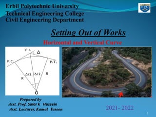
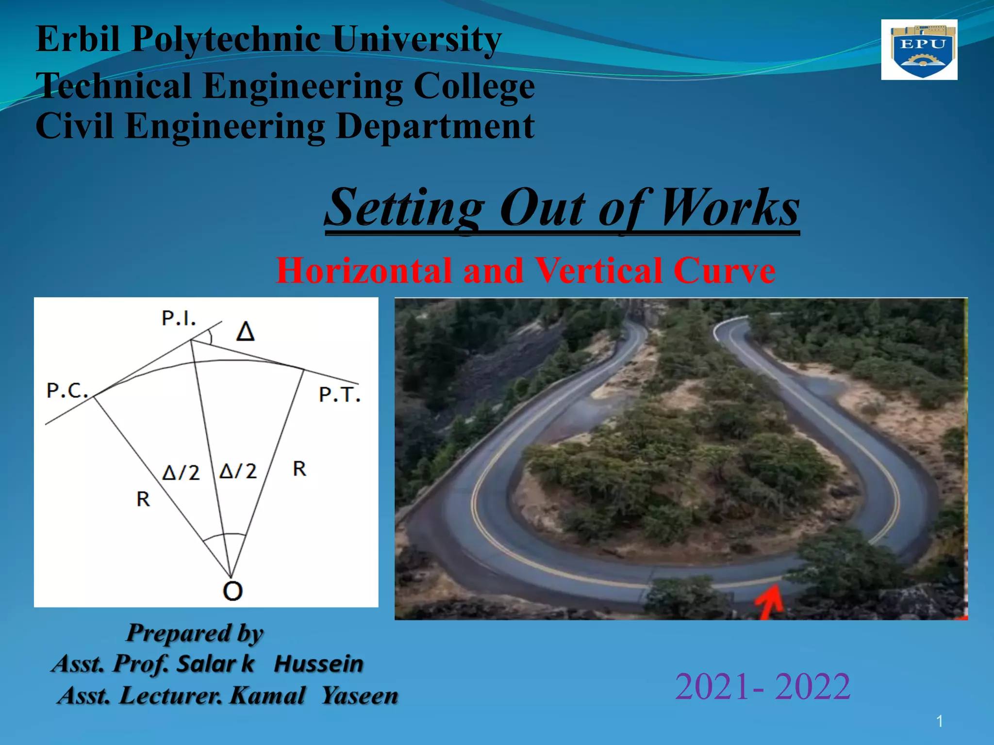
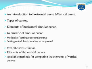
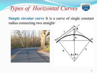
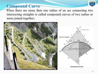
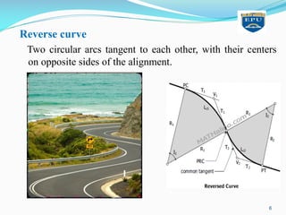
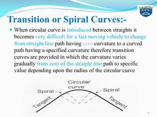
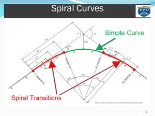
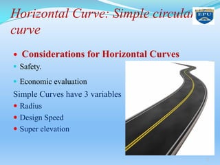
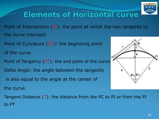
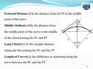
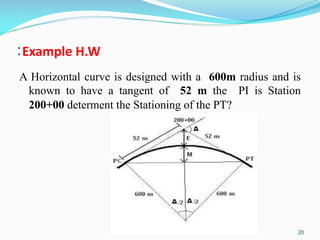
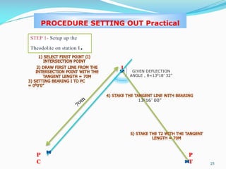
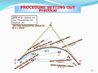
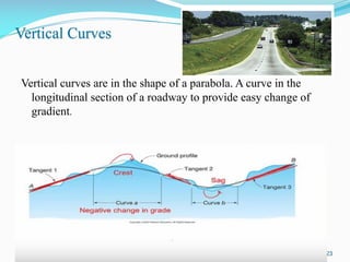


The document provides a comprehensive overview of horizontal and vertical curves in civil engineering, covering introduction, types, elements, and methods for setting out curves. It details horizontal curves like simple, compound, reverse, and transition curves, along with key formulas and examples. The document also addresses vertical curves, their significance, and practical calculations for their design related to road gradients.