This document discusses layout calculations for railway yards. It provides information on:
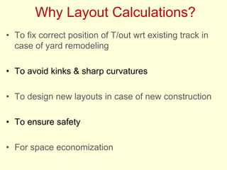
1) When layout calculations are needed, such as for yard remodeling, new construction projects, or rectifying defective layouts.
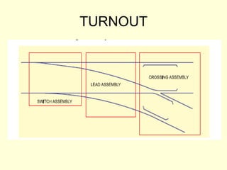
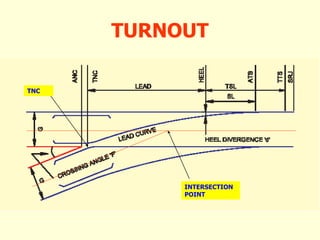
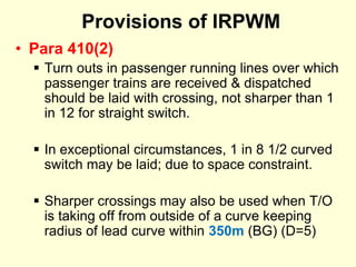
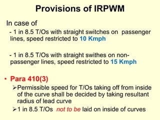
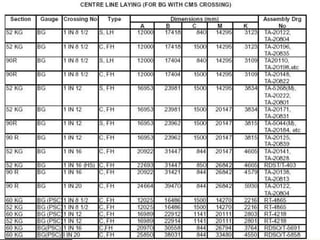
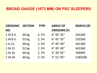
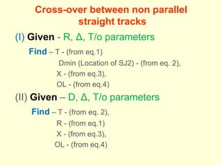
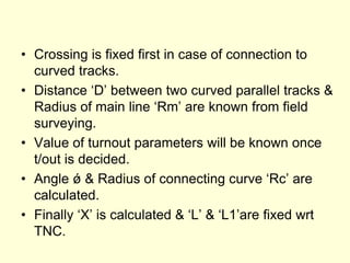
2) Key considerations for layout calculations including turnout parameters, permissible speeds and radii based on IRPWM guidelines.
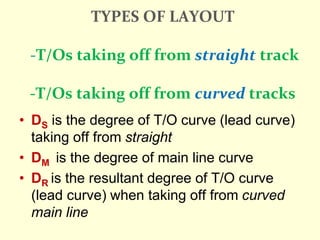
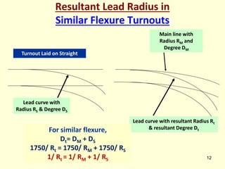
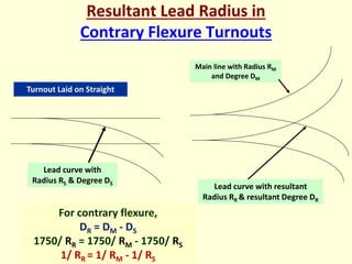
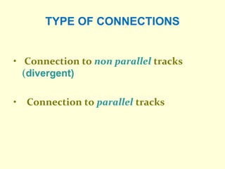
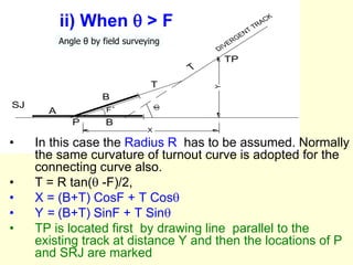
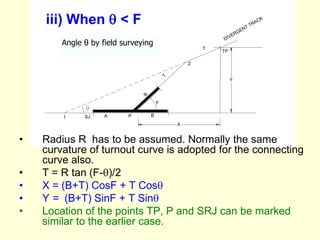
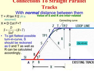
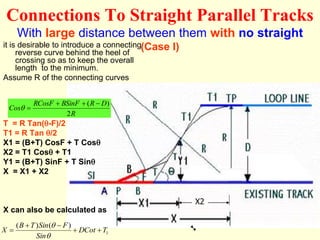
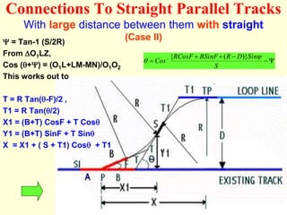
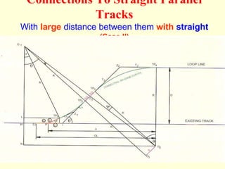
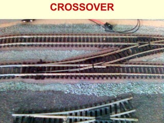
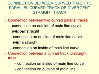
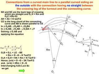
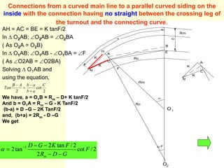
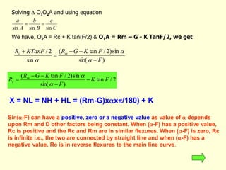
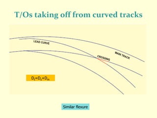
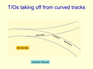
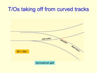
3) Methods for calculating layouts for different track connections including turnouts taking off from straight or curved tracks, connections to parallel and non-parallel tracks, crossovers, and connections between curved and straight tracks. Diagrams illustrate example calculations.
The document serves as a reference for engineers on best practices and regulatory guidelines for performing layout calculations to design efficient and safe railway yard track configurations.


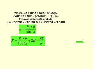
![Cross-over between curved parallel tracks
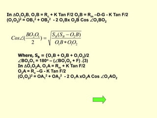
• In O1O2A, O1A = Rm + K Tan F/2
• O2A = Rc –G - K Tan F/2
• (O1O2)2 = (O1A)2 + (O2A)2 - 2 O1A xO2A Cos F
• = (Rm+KTanF/2) 2+ (Rc-G-KtanF/2) 2 -2(Rm+KTanF/2)
(Rc-G-KtanF/2)CosF ………..(1)
• In O1O2B, O1B = Rc + K Tan F/2
• O2B = Rm –D-G - K Tan F/2
• (O1O2) 2 = O1B2 + O2B2 - 2 O1Bx O2B Cos F
• = (Rc+KTanF/2) 2 +(Rm-D-G-KtanF/2) 2 -
2(Rc+KTanF/2) (Rm-D-G-KtanF/2)CosF ………..(2)
•
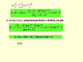
Equating equations (1) & (2), We can have,
)]
1
)}(
2
/
(
2
{
[
2
}]
)
2
/
(
){
2
(
2
)}
2
/
(
2
{
)}
2
/
(
2
}{
2
[{
CosF
F
KTan
G
DCosF
G
R
F
KTan
D
R
CosF
F
KTan
G
G
F
KTan
G
D
G
D
R
R m
m
m
c
](https://image.slidesharecdn.com/layoutcalculations1-231011180214-bd92b426/85/LAY-OUT-CALCULATIONS-1-pptx-46-320.jpg)

![11 Geometric Design of Railway Track [Vertical Alignment] (Railway Engineerin...](https://cdn.slidesharecdn.com/ss_thumbnails/geometricdesignofrailwaytrack-ii-200415172410-thumbnail.jpg?width=640&height=640&fit=bounds)


![10 Geometric Design of Railway Track [Horizontal Alignment] (Railway Engineer...](https://cdn.slidesharecdn.com/ss_thumbnails/geometricdesignofrailwaytrack-i-200415171932-thumbnail.jpg?width=640&height=640&fit=bounds)


