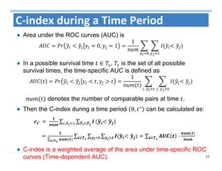
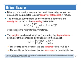
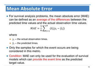
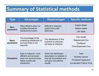
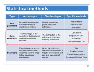
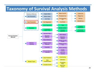
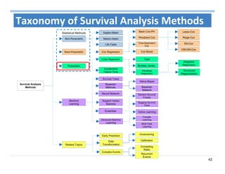
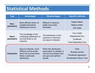
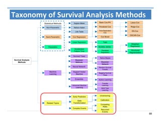
SlideShare a Scribd company logo
1
Machine Learning for 
Survival Analysis
Chandan K. Reddy
Dept. of Computer Science
Virginia Tech
http://www.cs.vt.edu/~reddy
Yan Li
Dept. of Computational Medicine
and Bioinformatics
Univ. of Michigan, Ann Arbor
2
Tutorial Outline
Basic Concepts
Statistical Methods
Machine Learning Methods
Related Topics
3
Tutorial Outline
Basic Concepts
Statistical Methods
Machine Learning Methods
Related Topics
4
Healthcare
Event
Prediction
Model
Demographics
Age
Gender
Race
Laboratory
Hemoglobin
Blood count
Glucose
Procedures
Hemodialysis
Contrast dye
Catheterization
Event of Interest : Rehospitalization; Disease recurrence; Cancer survival
Outcome: Likelihood of hospitalization within t days of discharge
Medications
ACE inhibitor
Dopamine
Milrinone
Comorbodities
Hypertension
Diabetes
CKD
IMPACT
Lower healthcare costs
Improve quality of life
5
Mining Events in Longitudinal Data
1 2 3 4 5 6 7 8 9 10 11 12
12345678910
Subjects
Time
- Death
- Dropout/Censored
- Other Events
Classification Problem:
3 +ve and 7 -ve
Cannot predict the time of event
Need to re-train for each time
Regression Problem:
Can predict the time of event
Only 3 samples (not 10)
– loss of data
Ping Wang, Yan Li, Chandan, K. Reddy, “Machine Learning for Survival
Analysis: A Survey”. ACM Computing Surveys (under revision), 2017.
6
Goal of survival analysis: To estimate the time to the event of
interest for a new instance 	with feature predictors denoted by .
Problem Statement
For a given instance , represented by a triplet , , .
is the feature vector;
is the binary event indicator, i.e.,	 	 1 for an uncensored instance
and 0	 for a censored instance;
denotes the observed time and is equal to the survival time for an
uncensored instance and for a censored instance, i.e.,
1
0
Note for :
The value of will be both non-negative and continuous.
is latent for censored instances.
7
Education
Financial
Event
Prediction
Model
Demographics
Age
Gender
Race/Ethnicity
Cash amount
Income
Scholarships
Enrollment
Transfer credits
College
Major
Event of Interest : Student dropout
Outcome: Likelihood of a student being dropout within t days
Semester
Semester GPA
% passed
% dropped
Pre-enrollment
High school GPA
ACT scores
Graduation age
IMPACT
Educated Society
Better Future
S. Ameri, M. J. Fard, R. B. Chinnam and C. K. Reddy, "Survival Analysis based Framework for Early Prediction of
Student Dropouts", CIKM 2016.
8
Crowdfunding
Projects
Duration
Goal amount
Category
Temporal
# Backers
Funding
# retweets
Event of Interest: Project Success
Outcome: Likelihood of a project being successful within t days
Event
Prediction
Model
Creators
Past success
Location
# projects
Twitter
# Promotions
Backings
Communities
IMPACT
Improve local economy
Successful businesses
Y. Li, V. Rakesh, and C. K. Reddy, "Project Success Prediction in Crowdfunding Environments", WSDM 2016.
9
Other Applications
How long ?
Event of interest
History information
Reliability: Device Failure Modeling in Engineering
Goal: Estimate when a device will fail
Features: Product and manufacturer details, user reviews
Duration Modeling: Unemployment Duration in Economics
Goal: Estimate the time people spend without a job (for getting a new job)
Features: User demographics and experience, Job details and economics
Click Through Rate: Computational Advertising on the Web
Goal: Estimate when a web user will click the link of the ad.
Features: User and Ad information, website statistics
Customer Lifetime Value: Targeted Marketing
Goal: Estimate the frequent purchase pattern for customers.
Features: Customer and store/product information.
10
Survival Analysis
Methods
Non-Parametric
Kaplan-Meier
Nelson-Aalen
Life-Table
Semi-Parametric
Basic Cox-PH
Penalized Cox
Time-Dependent
Cox
Cox Boost
Lasso-Cox
Ridge-Cox
EN-Cox
OSCAR-Cox
Cox Regression
Parametric
Linear Regression
Accelerated
Failure Time
Tobit
Buckley James
Panelized
Regression
Weighted
Regression
Structured
Regularization
Machine
Learning
Survival Trees
Ensemble
Advanced Machine
Learning
Bayesian
Network
Naïve Bayes
Bayesian
Methods
Support Vector
Machine
Random Survival
Forests
Bagging Survival
Trees
Active Learning
Transfer
Learning
Multi-Task
Learning
Early Prediction
Data
Transformation
Complex Events
Calibration
Uncensoring
Related Topics
Taxonomy of Survival Analysis Methods
Statistical Methods
Neural Network
Competing
Risks
Recurrent
Events
11
Tutorial Outline
Basic Concepts
Statistical Methods
Machine Learning Methods
Related Topics
12
Basics of Survival Analysis
Main focuses is on time to event data. Typically, survival data
are not fully observed, but rather are censored.
Several important functions:
Survival function, indicating the probability that the stance
instance can survive for longer than a certain time t.
Pr
Cumulative density function, representing the probability
that the event of interest occurs earlier than t.
1
Death density function:
⁄⁄
Hazard function: representing the probability the “event” of
interest occurs in the next instant, given survival to time t.
ln
Death
Cumulative hazard function
Survival function
exp	
Chandan K. Reddy and Yan Li, "A Review of Clinical Prediction Models", in Healthcare Data Analytics,
Chandan K. Reddy and Charu C. Aggarwal (eds.), Chapman and Hall/CRC Press, 2015.
13
Evaluation Metrics
Due to the presence of the censoring in survival data,
the standard evaluation metrics for regression such as
root of mean squared error and are not suitable for
measuring the performance in survival analysis.
Three specialized evaluation metrics for survival
analysis:
Concordance index (C-index)
Brier score
Mean absolute error
14
Concordance Index (C‐Index)
It is a rank order statistic for predictions against true outcomes
and is defined as the ratio of the concordant pairs to the total
comparable pairs.
Given the comparable instance pair , with and are the
actual observed times and S( ) and S( ) are the predicted
survival times,
The pair , is concordant if > and S( ) > S( ).
The pair , is discordant if > and S( ) < S( ).
Then, the concordance probability Pr 	
measures the concordance between the rankings of actual
values and predicted values.
For a binary outcome, C-index is identical to the area under the
ROC curve (AUC).
U. Hajime, et al. "On the C‐statistics for evaluating overall adequacy of risk prediction procedures with censored survival
data." Statistics in medicine, 2011.
15
Comparable Pairs
The survival times of two instances can be compared if:
Both of them are uncensored;
The observed event time of the uncensored instance is
smaller than the censoring time of the censored instance.
Without Censoring With Censoring
A total of 5C2 comparable pairs Comparable only with events and
with those censored after the events
H. Steck, B. Krishnapuram, C. Dehing-oberije, P. Lambin, and V. C. Raykar, “On ranking in survival analysis: Bounds on the
concordance index”, NIPS 2008.
16
C‐index
When the output of the model is the prediction of survival time:
̂ 	
1
|
:	:
Where | is the predicted survival probabilities,
denotes the total number of comparable pairs.
When the output of the model is the hazard ratio (Cox model):
̂ 	
1
:	:
Where · is the indicator function and is the estimated
parameters from the Cox based models. (The patient who has
a longer survival time should have a smaller hazard ratio).
17
C‐index during a Time Period
Area under the ROC curves (AUC) is
0, 1
1
In a possible survival time ∈ , is the set of all possible
survival times, the time-specific AUC is defined as 	
,
1
:	:	
denotes the number of comparable pairs at time .
Then the C-index during a time period 0, ∗ can be calculated as:
∗ 	 ∑ ∑:
∑ ∈
∑ ∑ ∑∈ ∑ ·∈
C-index is a weighted average of the area under time-specific ROC
curves (Time-dependent AUC).
18
Brier Score
Brier score is used to evaluate the prediction models where the
outcome to be predicted is either binary or categorical in nature.
The individual contributions to the empirical Brier score are
reweighted based on the censoring information:
1
denotes the weight for the instance.
The weights can be estimated by considering the Kaplan-Meier
estimator of the censoring distribution on the dataset.
/ 	
1/ 	
The weights for the instances that are censored before will be 0.
The weights for the instances that are uncensored at are greater than 1.
E. Graf, C. Schmoor, W. Sauerbrei, and M. Schumacher, “Assessment and comparison of prognostic classification schemes
for survival data”, Statistics in medicine, 1999.
19
Mean Absolute Error
For survival analysis problems, the mean absolute error (MAE)
can be defined as an average of the differences between the
predicted time values and the actual observation time values.
1
| |
where
-- the actual observation times.
-- the predicted times.
Only the samples for which the event occurs are being
considered in this metric.
Condition: MAE can only be used for the evaluation of survival
models which can provide the event time as the predicted
target value.
20
Summary of Statistical methods
Type Advantages Disadvantages Specific methods
Non-
parametric
More efficient when no
suitable theoretical
distributions known.
Difficult to interpret;
yields inaccurate
estimates.
Kaplan-Meier
Nelson-Aalen
Life-Table
Semi-
parametric
The knowledge of the
underlying distribution of
survival times is not
required.
The distribution of the
outcome is unknown;
not easy to interpret.
Cox model
Regularized Cox
CoxBoost
Time-Dependent Cox
Parametric
Easy to interpret, more
efficient and accurate
when the survival times
follow a particular
distribution.
When the distribution
assumption is violated, it
may be inconsistent and
can give sub-optimal
results.
Tobit
Buckley-James
Penalized regression
Accelerated Failure Time
21
Kaplan‐Meier Analysis 
Kaplan-Meier (KM) analysis is a nonparametric approach
to survival outcomes. The survival function is:
1
:	
E. Bradley. "Logistic regression, survival analysis, and the Kaplan-Meier curve." JASA 1988.
where
• … -- a set of distinct event times
observed in the sample.
• -- number of events at .
• -- number of censored observations
between and .
• -- number of individuals “at risk” right
before the death.
22
Survival Outcomes
Patient Days Status
1 21 1
2 39 1
3 77 1
4 133 1
5 141 2
6 152 1
7 153 1
8 161 1
9 179 1
10 184 1
11 197 1
12 199 1
13 214 1
14 228 1
Patient Days Status
15 256 2
16 260 1
17 261 1
18 266 1
19 269 1
20 287 3
21 295 1
22 308 1
23 311 1
24 321 2
25 326 1
26 355 1
27 361 1
28 374 1
Patient Days Status
29 398 1
30 414 1
31 420 1
32 468 2
33 483 1
34 489 1
35 505 1
36 539 1
37 565 3
38 618 1
39 793 1
40 794 1
Status
1: Death
2: Lost to follow up
3: Withdrawn Alive
23
Kaplan‐Meier Analysis
Kaplan-Meier Analysis
Time Status
1 21 1 1 0 40 0.975
2 39 1 1 0 39 0.95
3 77 1 1 0 38 0.925
4 133 1 1 0 37 0.9
5 141 2 0 1 36 .
6 152 1 1 0 35 0.874
7 153 1 1 0 34 0.849
1
:	
KM Estimator:
24
Kaplan‐Meier Analysis
KM Estimator:
Time Status ∑ Time Status ∑Estimate Sdv Error Estimate Sdv Error
1 21 1 0.975 0.025 1 40 21 287 3 . . 18 20
2 39 1 0.95 0.034 2 39 22 295 1 0.508 0.081 19 19
3 77 1 0.925 0.042 3 38 23 308 1 0.479 0.081 20 18
4 133 1 0.9 0.047 4 37 24 311 1 0.451 0.081 21 17
5 141 2 . . 4 36 25 321 2 . . 21 16
6 152 1 0.874 0.053 5 35 26 326 1 0.421 0.081 22 15
7 153 1 0.849 0.057 6 34 27 355 1 0.391 0.081 23 14
8 161 1 0.823 0.061 7 33 28 361 1 0.361 0.08 24 13
9 179 1 0.797 0.064 8 32 29 374 1 0.331 0.079 25 12
10 184 1 0.771 0.067 9 31 30 398 1 0.301 0.077 26 11
11 193 1 0.746 0.07 10 30 31 414 1 0.271 0.075 27 10
12 197 1 0.72 0.072 11 29 32 420 1 0.241 0.072 28 9
13 199 1 0.694 0.074 12 28 33 468 2 . . 28 8
14 214 1 0.669 0.075 13 27 34 483 1 0.206 0.07 29 7
15 228 1 0.643 0.077 14 26 35 489 1 0.172 0.066 30 6
16 256 2 . . 14 25 36 505 1 0.137 0.061 31 5
17 260 1 0.616 0.078 15 24 37 539 1 0.103 0.055 32 4
18 261 1 0.589 0.079 16 23 38 565 3 . . 32 3
19 266 1 0.563 0.08 17 22 39 618 1 0.052 0.046 33 2
20 269 1 0.536 0.08 18 21 40 794 1 0 0 34 1
25
Nelson‐Aalen Estimator
Nelson-Aalen estimator is a non-parametric estimator of the
cumulative hazard function (CHF) for censored data.
Instead of estimating the survival probability as done in KM
estimator, NA estimator directly estimates the hazard probability.
The Nelson-Aalen estimator of the cumulative hazard function:
-- the number of deaths at time
-- the number of individuals at risk at
The cumulative hazard rate function can be used to estimate the
survival function and its variance.
exp
The NA and KM estimators are asymptotically equivalent.
W. Nelson. “Theory and applications of hazard plotting for censored failure data.” Technometrics, 1972.
O. Aalen. “Nonparametric inference for a family of counting processes.” The Annals of Statistics, 1978.
26
Clinical Life Tables
Clinical life tables applies to grouped survival data from
studies in patients with specific diseases, it focuses more
on the conditional probability of dying within the interval.
The time interval is , VS.
… is a set of distinct death times
The survival function is:
1
KM analysis suits small data set with a more accurate analysis,
Clinical life table suit for large data set with a relatively approximate result.
Nonparametric
Assumption:
• at the beginning of each interval:	
• at the end of each interval:	
• on average halfway through the interval: /2
Cox, David R. "Regression models and life-tables", Journal of the Royal Statistical Society. Series B (Methodological), 1972.
27
Clinical Life Tables
Clinical Life Table
Interval
Interval
Start Time
Interval
End Time
Std. Error
of
1 0 182 40 1 39.5 8 0.797 0.06
2 183 365 31 3 29.5 15 0.392 0.08
3 366 548 13 1 12.5 8 0.141 0.06
4 549 731 4 1 3.5 1 0.101 0.05
5 732 915 2 0 2 2 0 0
1
Clinical Life Table:
NOTE:
The length of interval
is half year(183 days)
On average halfway through
the interval: /2
28
Statistical methods
Type Advantages Disadvantages Specific methods
Non-
parametric
More efficient when no
suitable theoretical
distributions known.
Difficult to interpret;
yields inaccurate
estimates.
Kaplan-Meier
Nelson-Aalen
Life-Table
Semi-
parametric
The knowledge of the
underlying distribution of
survival times is not
required.
The distribution of the
outcome is unknown;
not easy to interpret.
Cox model
Regularized Cox
CoxBoost
Time-Dependent Cox
Parametric
Easy to interpret, more
efficient and accurate
when the survival times
follow a particular
distribution.
When the distribution
assumption is violated, it
may be inconsistent and
can give sub-optimal
results.
Tobit
Buckley-James
Penalized regression
Accelerated Failure Time
29
Survival Analysis
Methods
Non-Parametric
Kaplan-Meier
Nelson-Aalen
Life-Table
Semi-Parametric
Basic Cox-PH
Penalized Cox
Time-Dependent
Cox
Cox Boost
Lasso-Cox
Ridge-Cox
EN-Cox
OSCAR-Cox
Cox Regression
Parametric
Linear Regression
Accelerated
Failure Time
Tobit
Buckley James
Panelized
Regression
Weighted
Regression
Structured
Regularization
Machine
Learning
Survival Trees
Ensemble
Advanced Machine
Learning
Bayesian
Network
Naïve Bayes
Bayesian
Methods
Support Vector
Machine
Random Survival
Forests
Bagging Survival
Trees
Active Learning
Transfer
Learning
Multi-Task
Learning
Early Prediction
Data
Transformation
Complex Events
Calibration
Uncensoring
Related Topics
Taxonomy of Survival Analysis Methods
Statistical Methods
Neural Network
Competing
Risks
Recurrent
Events
30
Cox Proportional Hazards Model
The Cox proportional hazards model is the most commonly
used model in survival analysis.
Hazard Function , sometimes called an instantaneous
failure rate, shows the event rate at time conditional on
survival until time or later.
, exp	 ⇒ 				log
,
where
• , , … , is the covariate vector.
• is the baseline hazard function, which can be an arbitrary
non-negative function of time.
The Cox model is a semi-parametric algorithm since the baseline
hazard function is unspecified.
D. R. Cox, “Regression models and life tables”. Journal of the Royal Statistical Society, 1972.
A linear model for the log
of the hazard ratio.
31
Cox Proportional Hazards Model
The Proportional Hazards assumption means that the hazard ratio of two
instances and is constant over time (independent of time).
,
,
exp	
exp	
exp	
The survival function in Cox model can be computed as follows:
exp exp 	
is the cumulative baseline hazard function;
exp represents the baseline survival function.
The Breslow’s estimator is the most widely used method to estimate ,
which is given by:
∑ ∈
if is an event time, otherwise 0.
represents the set of subjects who are at risk at time .
32
Optimization of Cox model
Not possible to fit the model using the standard likelihood function
Reason: the baseline hazard function is not specified.
Cox model uses partial likelihood function:
Advantage: depends only on the parameter of interest and is free of
the nuisance parameters (baseline hazard).
Conditional on the fact that the event occurs at , the individual
probability corresponding to covariate can be formulated as:
,
∑ ,∈
	 -- the total number of events of interest that occurred during
the observation period for instances.
⋯ -- the distinct ordered time to event of interest.
-- the covariate vector for the subject who has the event at .
-- the set of risk subjects at .
33
Partial Likelihood Function
The partial likelihood function of the Cox model will be:
exp	
∑ exp	∈
If	 1, the term in the product is the conditional probability;
if	 0, the corresponding term is 1, which means that the term will not
have any effect on the final product.
The coefficient vector is estimated by minimizing the negative
log-partial likelihood:
exp	
∈
The maximum partial likelihood estimator (MPLE) can be used
along with the numerical Newton-Raphson method to iteratively
find an estimator	 which minimizes .
D. R. Cox, Regression models and life tables, Journal of the Royal Statistical Society, 1972.
34
Regularized Cox Models
Regularized Cox regression methods:
	 ∗
							 is a sparsity inducing norm and is the regularization parameter.
Promotes Sparsity
Handles Correlation
Sparsity + Correlation
Adaptive Variants are
slightly more effective
Method Penalty Term Formulation
LASSO
Ridge
Elastic Net (EN) | | 1
Adaptive LASSO (AL) ∑ | |
Adaptive Elastic Net
(AEN)
| | 1
OSCAR ∥ ∥ ∥ ∥
Sparsity + Feature
Correlation Graph
35
Lasso‐Cox and Ridge‐Cox
Lasso performs feature selection and estimates the regression
coefficients simultaneously using a ℓ -norm regularizer .
Lasso-Cox model incorporates the ℓ -norm into the log-partial
likelihood and inherits the properties of Lasso.
Extensions of Lasso-Cox method:
Adaptive Lasso-Cox - adaptively weighted ℓ -penalties on regression
coefficients.
Fused Lasso-Cox - coefficients and their successive differences are
penalized.
Graphical Lasso-Cox - ℓ -penalty on the inverse covariance matrix is
applied to estimate the sparse graphs .
Ridge-Cox is Cox regression model regularized by a ℓ -norm
Incorporates a ℓ -norm regularizer to select the correlated features.
Shrink their values towards each other.
N. Simon et al., “Regularization paths for Coxs proportional hazards model via coordinate descent”, JSS 2011.
36
EN‐Cox and OSCAR‐Cox
EN-Cox method uses the Elastic Net penalty term (combining the ℓ
and squared ℓ penalties) into the log-partial likelihood function.
Performs feature selection and handles correlation between the features.
Kernel Elastic Net Cox (KEN-Cox) method builds a kernel similarity
matrix for the feature space to incorporate the pairwise feature
similarity into the Cox model.
OSCAR-Cox uses Octagonal Shrinkage and Clustering Algorithm for
Regression regularizer within the Cox framework.
β ∥ ∥ ∥ ∥
is the sparse symmetric edge set matrix from a graph constructed by
features.
Performs the variable selection for highly correlated features in regression.
Obtain equal coefficients for the features which relate to the outcome in
similar ways.
B. Vinzamuri and C. K. Reddy, "Cox Regression with Correlation based Regularization for Electronic Health Records", ICDM 2013.
37
CoxBoost
CoxBoost method can be applied to fit the sparse survival
models on the high-dimensional data by considers some
mandatory covariates explicitly in the model.
Similar goal: estimate the coefficients in Cox model.
Differences:
RGBA: updates in component-wise boosting or fits
the gradient by using all covariates in each step.
CoxBoost: considers a flexible set of candidate
variables for updating in each boosting step.
H. Binder and M. Schumacher, “Allowing for mandatory covariates in boosting estimation of sparse high-dimensional survival
models”, BMC bioinformatics, 2008.
CoxBoost VS. Regular gradient boosting approach (RGBA)
38
CoxBoost
How to update in each iteration of CoxBoost?
Assume that , ⋯ , being the actual
estimate of the overall parameter vector after step 	
	1	of the algorithm and predefined candidate sets of
features in step with ⊂ 1, ⋯ , , 1, ⋯ , .
Component-wise CoxBoost: 1 , ⋯ , in each step .
Update all parameters
in each set
simultaneously (MLE)
Determine Best ∗
which improves the
overall fitting most
	 		 ∈ ∗
	 ∉ ∗
Update
Special case:
39
TD‐Cox Model
Cox regression model is also effectively adapted to time-
dependent Cox model to handle time-dependent covariates.
Given a survival analysis problem which involves both time-
dependent and time-independent features, the variables at
time can be denoted as:
⋅	 , ⋅	 , … , ⋅	 , ⋅	 , ⋅ , … , ⋅	 	
The TD-Cox model can be formulated as:
, exp	 · ·
Time-dependent Time-independent
40
TD‐Cox Model
For the two sets of predictors at time :
,	 , … , , , , … ,
		 ,	 , … , , ⋅		
∗
, ⋅		
∗
, … , 	
The hazard ratio for TD-Cox model can be computed as
follows:
,
,
Since the first component in the exponent is time-dependent, we can
consider the hazard ratio in the TD-Cox model as a function of time .
This means that it does not satisfy the PH assumption mentioned in
the standard Cox model.
41
Counting Process Example
ID
Gende
r
(0/1)
Weight
(lb)
Smoke
(0/1)
Start Time
(days)
Stop Time
(days) Status
1 (F) 125 0 0 20 1
0 (M) 171 1 0 20 0
0 180 0 20 30 1
0 165 1 0 20 0
0 160 0 20 30 0
0 168 0 30 50 0
1 130 0 0 20 0
1 125 1 20 30 0
1 120 1 30 80 1
42
Survival Analysis
Methods
Non-Parametric
Kaplan-Meier
Nelson-Aalen
Life-Table
Semi-Parametric
Basic Cox-PH
Penalized Cox
Time-Dependent
Cox
Cox Boost
Lasso-Cox
Ridge-Cox
EN-Cox
OSCAR-Cox
Cox Regression
Parametric
Linear Regression
Accelerated
Failure Time
Tobit
Buckley James
Panelized
Regression
Weighted
Regression
Structured
Regularization
Machine
Learning
Survival Trees
Ensemble
Advanced Machine
Learning
Bayesian
Network
Naïve Bayes
Bayesian
Methods
Support Vector
Machine
Random Survival
Forests
Bagging Survival
Trees
Active Learning
Transfer
Learning
Multi-Task
Learning
Early Prediction
Data
Transformation
Complex Events
Calibration
Uncensoring
Related Topics
Taxonomy of Survival Analysis Methods
Statistical Methods
Neural Network
Competing
Risks
Recurrent
Events
43
Statistical Methods
Type Advantages Disadvantages Specific methods
Non-
parametric
More efficient when no
suitable theoretical
distributions known.
Difficult to interpret;
yields inaccurate
estimates.
Kaplan-Meier
Nelson-Aalen
Life-Table
Semi-
parametric
The knowledge of the
underlying distribution of
survival times is not
required.
The distribution of the
outcome is unknown;
not easy to interpret.
Cox model
Regularized Cox
CoxBoost
Time-Dependent Cox
Parametric
Easy to interpret, more
efficient and accurate
when the survival times
follow a particular
distribution.
When the distribution
assumption is violated, it
may be inconsistent and
can give sub-optimal
results.
Tobit
Buckley-James
Penalized regression
Accelerated Failure Time
44
Parametric Censored Regression
Survival function Pr : the probability that the event did
not happen up to time
— ∏ , : The joint probability of censored instances.
 Likelihood function
, ,
0.2
0.4
0.6
0.8
0
1 2 3yi
f(t)
yi
S(t)
Event density function : rate of events per unit time
— ∏ , : The joint probability of uncensored instances.
45
Parametric Censored Regression
Generalized Linear Model
														 ~
Where
																													 																		 	
log	 	 	 	
/ 1
Negative log-likelihood
m
,
2
log log log 1
Uncensored
Instances
censored
Instances
46
Optimization
Use second order second-order Taylor expansion to formulate the
log-likelihood as a reweighted least squares
where , . The first-order derivative , second-
order derivative , and other components in optimization share the
same formulation with respect to · , · , · ,	and		F · .
In addition, we can add some regularization term to encode some
prior assumption.
Y. Li, K. S. Xu, C. K. Reddy, “Regularized Parametric Regression for High-dimensional Survival Analysis“, 2016. SDM
47
Pros and Cons
Advantages:
Easy to interpret.
Rather than Cox model, it can directly predict the
survival(event) time.
More efficient and accurate when the time to event of
interest is follow a particular distribution.
Disadvantages:
The model performance strongly relies on the choosing of
distribution, and in practice it is very difficult to choose a
suitable distribution for a given problem.
Li, Yan, Vineeth Rakesh, and Chandan K. Reddy. "Project success prediction in crowdfunding environments."
Proceedings of the Ninth ACM International Conference on Web Search and Data Mining. ACM, 2016.
48
Commonly Used Distributions
Distributions PDF Survival Hazard
Exponential exp	 exp	
Weibull exp	 exp	
Logistic
/
1 /
/
1 /
1
1 /
Log-logistic
1
1
1 1
Normal
1
2
exp	
2
1 Φ
1
2 1 Φ
exp	
2
Log-normal
1
2
exp	
log	
2
1 Φ
log	 1
2
exp	
log	
2
1 Φ
log
49
Tobit Model
Tobit model is one of the earliest attempts to extend linear regression
with the Gaussian distribution for data analysis with censored
observations.
In Tobit model, a latent variable ∗ is introduced and it is assumed to
linearly depend on as:
y∗
	 , ∼ 	 0,
where 	is a normally distributed error term.
For the instance, the observable variable will be ∗
if ∗
0,
otherwise it will be 0. This means that if the latent variable is above
zero, the observed variable equals to the latent variable and zero
otherwise.
The parameters in the model can be estimated with maximum
likelihood estimation (MLE) method.
J. Tobin, Estimation of relationships for limited dependent variables. Econometrica: Journal of the Econometric Society, 1958.
50
Buckley‐James Regression Method
The Buckley-James (BJ) regression is a AFT model.
log	
The estimated target value
log ∗ log 																																																	 1
log | log log , 0
J. Buckley and I. James, Linear regression with censored data. Biometrika, 1979.
1
0
The key point is to calculate log | log log , :
log | log log , log
·
1 log
Rather than a selected closed formed theoretical distribution, the Kaplan-Meier
(KM) estimation method are used to approximate the F(·).
51
The Elastic-Net regularizer also has been used to penalize the BJ-
regression (EN-BJ) to handle the high-dimensional survival data.
To estimate of of BJ and EN-BJ models, we just need to calculate
log ∗
based on the of pervious iteration and then minimize the lest
square or penalized lest square via standard algorithms.
Buckley‐James Regression Method
The Least squares is used as the empirical loss function
min
1
2
log ∗
Where log ∗
= log
1 ·
1 log
min
1
2
log ∗
	 1 	
1
2
	
2
2
Wang, Sijian, et al. “Doubly Penalized Buckley–James Method for Survival Data with High‐Dimensional Covariates.” Biometrics, 2008
52
Regularized Weighted Linear Regression
Induce more penalize to case 1 and less penalize to case 2
×
✓
Y. Li, B. Vinzamuri, and C. K. Reddy, “Regularized Weighted Linear Regression for High-dimensional Censored Data“, SDM 2016.
53
Weighted Residual Sum‐of‐Squares
More weight to the censored instances whose estimated
survival time is lesser than censored time
Less weight to the censored instances whose estimated
survival time is greater than censored time.
where weight is defined as follows:
=
1			 		 1																												
		 			 		 0		 			
		0			 		 0		 			
A demonstration of linear
regression model for dataset with
right censored observations.
Weighted residual sum-of-squares
1
2
54
Self‐Training Framework
Training
a base
model
Estimate
survival
time
Approximate
the survival
time of
censored
instances
Update
training
set
If the estimated survival
time is larger than censored
time
Stop when the
training dataset won’t
change
Self-training: training the model by using its own prediction
55
Bayesian Survival Analysis
Bayesian Paradigm
Based on observed data , one can build a likelihood function | .
(likelihood estimator)
Suppose is random and has a prior distribution denote by .
Inference concerning is based on the posterior distribution
usually does not have an analytic closed form, requires methods
like MCMC to sample from | and methods to estimate .
Posterior predictive distribution of a future observation vector given D
where | denotes the sampling density function of
Penalized regression encode assumption via regularization term,
while Bayesian approach encode assumption via prior distribution.
Ibrahim, Joseph G., Ming‐Hui Chen, and Debajyoti Sinha. Bayesian survival analysis. John Wiley & Sons, 2005.
56
Bayesian Survival Analysis
Under the Bayesian framework the lasso estimate can be viewed as a
Bayesian posterior mode estimate under independent Laplace priors for
the regression parameters.
Komarek, Arnost. Accelerated failure time models for multivariate interval-censored data with
flexible distributional assumptions. Diss. PhD thesis, PhD thesis, Katholieke Universiteit
Leuven, Faculteit Wetenschappen, 2006.
Lee, Kyu Ha, Sounak Chakraborty, and Jianguo Sun. "Bayesian variable selection in
semiparametric proportional hazards model for high dimensional survival data." The
International Journal of Biostatistics 7.1 (2011): 1-32.
Similarly based on the mixture representation of Laplace distribution, the
Fused lasso prior and group lasso prior can be also encode based on a
similar scheme.
Lee, Kyu Ha, Sounak Chakraborty, and Jianguo Sun. "Survival prediction and variable
selection with simultaneous shrinkage and grouping priors." Statistical Analysis and Data
Mining: The ASA Data Science Journal 8.2 (2015): 114-127.
A similar approach can also be applied in the parametric AFT model.
57
Deep Survival Analysis
Deep Survival Analysis is a hierarchical generative approach to
survival analysis in the context of the EHR
Deep survival analysis models covariates and survival time in a
Bayesian framework.
It can easily handle both missing covariates and model survival time.
Deep exponential families (DEF) are a class of multi-layer probability
models built from exponential families. Therefore, they are capable
to model the complex relationship and latent structure to build a joint
model for both the covariates and the survival times.
R. Ranganath, A. Perotte, N. Elhadad, and D. Blei. "Deep survival analysis." Machine Learning for Healthcare, 2016.
is the output of DEF network, which can be used to generate the
observed covariates and the time to failure.
58
Deep Survival Analysis
is the feature vector, which is supposed can be generated from a prior
distribution.
The Weibull distribution is used to model the survival time.
a and b are drawn from normal distribution, they are parameter related to
survival time.
Given a feature vector x, the model makes predictions via the posterior
predictive distribution:
59
Tutorial Outline
Basic Concepts
Statistical Methods
Machine Learning Methods
Related Topics
60
Machine Learning Methods
Basic ML Models
Survival Trees
Bagging Survival Trees
Random Survival Forest
Support Vector Regression
Deep Learning
Rank based Methods
Advanced ML Models
Active Learning
Multi-task Learning
Transfer Learning
61
Survival Tree
Survival trees is similar to decision tree which is built by recursive
splitting of tree nodes. A node of a survival tree is considered
“pure” if all the patients in the node survive for an identical span of
time.
The logrank test is most commonly used dissimilarity measure that
estimates the survival difference between two groups. For each
node, examine every possible split on each feature, and then
select the best split, which maximizes the survival difference
between two children nodes.
LeBlanc, M. and Crowley, J. (1993). Survival Trees by Goodness of Split. Journal of the American Statistical
Association 88, 457–467.
62
Logrank Test
∑ /
∑
 the numerator is the squared sum of deviations between the observed
and expected values. The denominator is the variance of the
(Patnaik ,1948).
 The test statistic, , gets bigger as the differences between the
observed and expected values get larger, or as the variance gets smaller.
 It follows a distribution asymptotically under the null hypothesis.
The logrank test is obtained by constructing a (2 X 2) table at each distinct
death time, and comparing the death rates between the two groups,
conditional on the number at risk in the groups. Let , … , 	represent the
ordered, distinct death times. At the -th death time, we have the following:
Segal, Mark Robert. "Regression trees for censored data." Biometrics (1988): 35-47.
63
Bagging Survival Trees
- Draw B bootstrap samples from the original data.
- Grow a survival tree for each bootstrap sample based on all features.
Recursively spitting the node using the feature that maximizes survival
difference between daughter nodes.
- Compute the bootstrap aggregated survival function for a new observation
.
Bagging
Survival
Tree
Bagging
Survival
Trees
Hothorn, Torsten, et al. "Bagging survival trees." Statistics in medicine 23.1 (2004): 77-91.
Bagging
Survival
Trees
The samples in the selected
leaf node of 1-st Tree
The samples in the selected
leaf node of B-th Tree
…
Build K-M curve
An aggregated
estimator of | )
64
Random Survival Forests
1. Draw B bootstrap samples from the original data (63% in the bag data,
37% Out of bag data(OOB)).
2. Grow a survival tree for each bootstrap sample based on randomly
select candidate features, and splits the node using feature from the
selected candidate features that maximizes survival difference between
daughter nodes.
3. Grow the tree to full size, each terminal node should have no less than
0 unique deaths.
4. Calculate a Cumulative Hazard Function (CHF) for each tree. Average
to obtain the bootstrap ensemble CHF.
5. Using OOB data, calculate prediction error for the OOB ensemble CHF.
Random
Forests
Survival
Tree RSF
H. Ishwaran, U. B. Kogalur, E. H. Blackstone and M. S. Lauer, “Random Survival Forests”. Annals of
Applied Statistics, 2008
65
Random Survival Forests
The cumulative hazard function (CHF) in random survival forests is
estimated via Nelson-Aalen estimator:
,
,
,
where , is the -th distinct event time of the samples in leaf , , is the
number events at , , and , is the number of individuals at risk at , .
OOB ensemble CHF ( ∗∗
) and bootstrap ensemble CHF ( ∗
)
∗∗
∑ ,
∗
|
∑ ,
, 											 ∗
1 ∗
|
where ∗
| is the CHF of the node in b-th bootstrap which belongs to.
, 1 if i is an OOB case for b; otherwise, set , 0. Therefore OOB
ensemble CHF is the average over bootstrap samples which i is OOB, and
bootstrap ensemble CHF is the average of all B bootstrap.
O. O. Aalen, “Nonparametric inference for a family of counting processes”, Annals of Statistics 1978.
66
Support Vector Regression (SVR)
Once a model has been learned, it can be applied to a new instance
through
is a kernel, and the SVR algorithm can abstractly be
considered as a linear algorithm
	 : margin of error
C: regularization parameter
: slack variables
67
Support Vector Approach for Censored Data
)( ixfiI iU
),),(( iii UIxfc
Graphical representation of Loss functions
)( ixfiI iU
),),(( iii UIxfc
SVR loss SVRC loss in general SVRC loss for right
censored
∞
Interval Targets: These are samples for which we have both an upper and a
lower bound on the target. The tuple ( , , ) with < .
As long as the output is between and , there is no empirical error.
Right censored sample is written as ( , ∞) whose survival time is
greater than ∈ , but the upper bound is unknown.
P. K. Shivaswamy, W. Chu, and M. Jansche. "A support vector approach to censored targets”, ICDM 2007.
68
Support Vector Regression for Censored Data 
A graphical representation of the SVRc parameters for events.
Graphical representation of the SVRc parameters for censored data.
Greater acceptable margin when the predicted
value is greater than the censored time
Less penalty rate when the predicted value is
greater than the censored time
The possible survival time of censored instances
should be grater than or equal to the corresponding
censored time.
Lesser acceptable margin when the predicted
value is grater than the event time
Greater penalty rate when the predicted value is
greater than the censored time
Predicting a high risky patient will survive longer is
more gangrenous than predicting a low risky patient
will survive shorter
F. M. Khan and V. B. Zubek. "Support vector regression for censored data (SVRc): a novel tool for survival
analysis." ICDM 2008
69
Neural Network Model
Hidden layer takes softmax , as active function.
D. Faraggi and R. Simon. "A neural network model for survival data." Statistics in medicine, 1995.
Softmax
function
1
...
Input layer Hidden layer Output layer
Cox Proportional
Hazards Model
,
:
,
:
No longer to be a linear function
70
Deep Survival: A Deep Cox Proportional Hazards Network
Takes some modern deep learning techniques such as Rectified
Linear Units (ReLU) active function, Batch Normalization, dropout.
Katzman, Jared, et al. "Deep Survival: A Deep Cox Proportional Hazards Network." arXiv , 2016.
1
...Input layer Hidden layers
Output layer
Cox Proportional
Hazards Model
...
. . .
,
:
,
:
No longer to be a linear function
71
Deep Convolutional Neural Network
: image patch from -th patient
: the deep model
X. Zhu, J. Yao, and J. Huang. "Deep convolutional neural network for survival analysis with pathological images“, BIBM 2016.
Pos: Directly built deep model for survival analysis from images input
,
:
,
:
No longer to be a liner
function
72
Ranking based Models
C-index is a pairwise ranking based evaluation metric. Boosting
concordance index (BoostCI) is an approach which aims at directly optimize
the C-index.
is the kaplan-Meier estimator, and as the existence of · the above
definition is non-smooth and nonconvex, which is hart to optimize.
In BoostCI, a sigmoid function is used to provide a smooth approximation
for indicator function.
Therefore, we have the smoothed version
weights
A. Mayr and M. Schmid, “Boosting the concordance index for survival data–a unified framework to derive and evaluate
biomarker combinations”, PloS one, 2014.
73
BoostCI Algorithm
The component-wise gradient boosting algorithm is used to
optimize the smoothed C-index.
Learning Step:
1. Initialize the estimate of the marker combination with offset values,
and set maximum number ( ) of iteration, and set 1.
2. Compute the negative gradient vector of smoothed C-index.
3. Fit the negative gradient vector separately to each of the components of
via the base-learners :, .
4. Select the component that best fits the negative gradient vector, and the
selected index of base-learn is denote as ∗
5. Update the marker combination for this component
6. Stop if . Else increase by one and go back to step 2
← ∗ :, ∗ .
74
Machine Learning Methods
Basic ML Models
Survival Trees
Bagging Survival Trees
Random Survival Forest
Support Vector Machine
Deep Learning
Rank based Methods
Advanced ML Models
Active Learning
Multi-Task Learning
Transfer Learning
75
Active Learning for Survival Data
Objective: Identify the representative samples in the data
Active learning based framework for the survival regression using a novel
model discriminative gradient based sampling procedure.
Helps clinicians to understand more about the most representative patients.
B. Vinzamuri, Y. Li, C. Reddy, "Active Learning Based Survival Regression for Censored Data", CIKM 2014.





K
k
X
k
poolX
L
XThX
1
)(
)|(maxarg


Outcome: Allow the Model to select instances
to be included. It can minimize the training
cost and complexity of the model and obtain a
good generalization performance for Censored
data.
Our sampling method chooses that particular
instance which maximizes the following
criterion.
76
EHR
features(X)
Censored
Status(δ)
Time to
Event(T)
Column
wise kernel
matrix(Ke)
Partial log
likelihood L(β)
Compute
Gradient
δL(β)/ δβ
Output
Survival AUC
and RMSE
Unlabelled
Pool (Pool)
Domain Expert
(Oracle)
Train Cox Model
Elastic Net
Regularization
Gradient Based
Discriminative
Sampling
End of active
learning
rounds
Labelling
request for
instance
Update
Training
data
Active Learning with Censored Data
77
Multi‐task Learning Formulation
Y 1 2 3 4 5 6 7 8 9 10 11 12
1 1 1 1 1 1 1 1 1 1 0 0 0
2 1 1 1 1 1 ? ? ? ? ? ? ?
3 1 1 1 1 1 1 1 1 1 1 ? ?
4 1 1 1 0 0 0 0 0 0 0 0 0
0 6 12
Month
1
4
3
2
 Similar tasks: All the binary classifiers aim at predicting the life status
of each patient.
 Temporal smoothness: For each patient, the life statuses of adjacent
time intervals are mostly same.
 Not reversible: Once a patient is dead, he is impossible to be alive
again.
1: Alive 0: Death ?: Unknown
Advantage: The model is general, no assumption on either survival
time or survival function.
patient
78
Multi‐task Learning Formulation
Y 1 2 3 4 5 6 7 8 9 10 11 12
D1 1 1 1 1 1 1 1 1 1 0 0 0
D2 1 1 1 1 1 ? ? ? ? ? ? ?
D3 1 1 1 1 1 1 1 1 1 1 ? ?
D4 1 1 1 0 0 0 0 0 0 0 0 0
How to deal with the “?” in Y
W 1 2 3 4 5 6 7 8 9 10 11 12
D1 1 1 1 1 1 1 1 1 1 1 1 1
D2 1 1 1 1 1 0 0 0 0 0 0 0
D3 1 1 1 1 1 1 1 1 1 1 0 0
D4 1 1 1 1 1 1 1 1 1 1 1 1
The Proposed objective function:
min
∈
1
2
Π
2 ,
Where
Π
1
0 0
Yan Li, Jie Wang, Jieping Ye and Chandan K. Reddy “A Multi-Task Learning Formulation for Survival Analysis". KDD 2016
Y and should follow a non-negative non-increasing list structure
0, | , ∀ 1, … , , ∀ 1, … ,
Similar tasks: select some common features across all the task via , -norm.
Handling
Censored
Temporal smoothness & Irreversible:
79
min
∈
Π
min
∈ 2 ,
2
Multi‐task Learning Formulation
min
∈
1
2
Π
2 ,
Subject to:
ADMM:
min
∈
1
2
Π
2 ,
Solving the  , ‐norm by using FISTA algorithm
Solving the non‐negative non‐increasing list structure by max‐heap projection
An adaptive variant model
Too many time intervals, non-negative non-increasing list will be so
strong that will overfit the model. Relaxation of the above model:
80
Multi‐Task Logistic Regression
Model survival distribution via a sequence of dependent regressions.
Consider a simpler classification task of predicting whether an individual
will survive for more than months.
C. Yu et al. "Learning patient-specific cancer survival distributions as a sequence of dependent regressors." NIPS 2011.
Consider a serious of time points ( , , , … , ), we can get a series of
logistic regression models
The model should enforce the dependency of the outputs by predicting the
survival status of a patient at each of the time snapshots, let
( , , , … , ) where 0 (no death event yet ), and 1 (death)
81
Multi‐Task Logistic Regression
A very similar idea as cox model:
exp ∑ :, exp ∑ :, with 1	∀	
1, … , .
is the score of sequence with the event occurring in the interval
, . But different from cox model the coefficient is different in
different time interval. So no proportional hazard assumption.
For censored instances:
The numerator is the score of the death will happen after
In the model add ∑ :, :, regularization term to
achieve temporary smoothness.
82
Knowledge Transfer 
Transfer learning models aim at using auxiliary data to
augment learning when there are insufficient number of training
samples in target dataset.
Traditional Machine
Learning
Transfer Learning
training items
Learning System Learning System
Learning System
Learning SystemKnowledge
×
Similar but
not the
same
83
Transfer Learning for Survival Analysis
Source data
Target data
X B
…
Source Task
Target Task
• Both source and target tasks are survival analysis problem.
• There exist some features which are important among all correlated disease.
Yan Li, Lu Wang, Jie Wang, Jieping Ye and Chandan K. Reddy "Transfer Learning for Survival Analysis via Efficient L2,1-norm
Regularized Cox Regression". ICDM 2016.
Labeling the time-to-event data is very time consuming!
How long ? Event of interestHistory information
TCGA
84
Transfer‐Cox Model
The Proposed objective function:
min
,
1
2 ,
Where , , , and denote the coefficient
vector and negative partial log-likelihood,
log 	 β 	
ᵢ
,
of source take and target take, respectively. And
, .
• L2,1 norm can encourage group sparsity; therefore, it
selects some common features across all the task.
• We propose a FISTA based algorithm to solve the
problem with a linear scalability.
85
Using Strong Rule in Learning Process
Theorem: Given a sequence of
parameter values
⋯ and suppose the
optimal solution 1 at is
known. Then for any 1, 2, … , m
the feature will be discarded if
1 2
and the corresponding coefficient
will be set to 0
Let B=0, Calculate =
Let K=k+1, Calculate
Discard inactive features
based on Theorem
Using FISTA algorithm
update result
Check KKT condition Update selected
active features
All selected
feature
obey KKT
Record optimal
solution
86
Summary of Machine Learning Methods
Basic ML Models
Survival Trees
Bagging Survival Trees
Random Survival Forest
Support Vector Regression
Deep Learning
Rank based Methods
Advanced ML Models
Active Learning
Multi-Task Learning
Transfer Learning
87
Tutorial Outline
Basic Concepts
Statistical Methods
Machine Learning Methods
Related Topics
88
Survival Analysis
Methods
Non-Parametric
Kaplan-Meier
Nelson-Aalen
Life-Table
Semi-Parametric
Basic Cox-PH
Penalized Cox
Time-Dependent
Cox
Cox Boost
Lasso-Cox
Ridge-Cox
EN-Cox
OSCAR-Cox
Cox Regression
Parametric
Linear Regression
Accelerated
Failure Time
Tobit
Buckley James
Panelized
Regression
Weighted
Regression
Structured
Regularization
Machine
Learning
Survival Trees
Ensemble
Advanced Machine
Learning
Bayesian
Network
Naïve Bayes
Bayesian
Methods
Support Vector
Machine
Random Survival
Forests
Bagging Survival
Trees
Active Learning
Transfer
Learning
Multi-Task
Learning
Early Prediction
Data
Transformation
Complex Events
Calibration
Uncensoring
Related Topics
Taxonomy of Survival Analysis Methods
Statistical Methods
Neural Network
Competing
Risks
Recurrent
Events
89
Related Topics
Early Prediction
Data Transformation
Uncensoring
Calibration
Complex Events
Competing Risks
Recurrent Events
90
Early Stage Event PredictionSubjects
S1
S5
S4
S3
S2
S6
tc tfTime
M. J Fard, P. Wang, S. Chawla, and C. K. Reddy, “A Bayesian perspective on early stage event prediction in longitudinal data”,
TKDE 2016.
Any existing survival model can predict only until tc
Develop a Bayesian approach for early stage prediction.
Collecting data for survival analysis is very “time” consuming.
91
Bayesian Approach
Naïve Bayes (NB)
Tree-Augmented
Naïve Bayes (TAN)
Bayesian Networks
(BN)
   

m
j cj tyxP1
1|      

m
j pcj jxtyxP1
,1|      

m
j jcj xPatyxP1
,1|
Probability of
Event Occurrence
    f
ff
ttxP
LikelihoodX
ttxtyP


,
Prior
,|1
   a
b
ct
etFWeibull c

1:
 
  a
b
tc
c
tF 


1
1
:logistic-Log
Extrapolation of Prior
92
Percentage of available event occurrence information
20% 40% 60% 80% 100%
Accuracy
0.9
0.88
0.86
0.74
0.82
0.76
0.84
0.8
0.78
0.72
0.7
Cox
LR
RF
NB
TAN
BN
ESP_NB
ESP_TAN
ESP_BN
Percentage of available event occurrence information
20% 40% 60% 80% 100%
Accuracy
0.9
0.88
0.86
0.74
0.82
0.76
0.84
0.8
0.78
0.72
0.7
Cox
LR
RF
NB
TAN
BN
ESP_NB
ESP_TAN
ESP_BN
Percentage of available event occurrence information
20% 40% 60% 80% 100%
Accuracy
0.9
0.88
0.86
0.74
0.82
0.76
0.84
0.8
0.78
0.72
0.7
Cox
LR
RF
NB
TAN
BN
ESP_NB
ESP_TAN
ESP_BN
Percentage of available event occurrence information
20% 40% 60% 80% 100%
Accuracy
0.9
0.88
0.86
0.74
0.82
0.76
0.84
0.8
0.78
0.72
0.7
Cox
LR
RF
NB
TAN
BN
ESP_NB
ESP_TAN
ESP_BN
Percentage of available event occurrence information
20% 40% 60% 80% 100%
Accuracy
0.9
0.88
0.86
0.74
0.82
0.76
0.84
0.8
0.78
0.72
0.7
Cox
LR
RF
NB
TAN
BN
ESP_NB
ESP_TAN
ESP_BN
Early Stage Prediction
93
Data Transformation
Two data transformation techniques that will be useful
for data pre-processing in survival analysis.
Uncensoring approach
Calibration
Transform the data to a more conducive form so that
other survival-based (or sometimes even the standard
algorithms) can be applied effectively.
94
Uncensoring Approach
The censored instances actually have partial informative
labeling information which provides the possible range of
the corresponding true response (survival time).
Such censored data have to be handled with special
care within any machine learning method in order to
make good predictions.
Two naive ways of handling such censored data:
Delete the censored instances.
Treating censoring as event-free.
95
Uncensoring Approach I
For each censored instance, estimate the probability of event and probability
of being censored (considering censoring as a new event) using Kaplan-
Meier estimator. Give a new class label based on these probability values.
M. J Fard, P. Wang, S. Chawla, and C. K. Reddy, “A bayesian perspective on early stage event prediction in longitudinal data”,
TKDE 2016.
Probability of un-censoringProbability of survival
Probability of event Probability of censoring
Event-freeEvent
1
: 	
1
∗
:
1 1
Yes No
96
Uncensoring Approach II
Group the instances in the given data into three categorizes:
(i) Instances which experience the event of interest during the
observation will be labeled as event.
(ii) Instances whose censored time is later than a predefined time
point are labeled as event-free.
(iii) Instances whose censored time is earlier than a predefined
time point,
A copy of these instances will be labeled as event.
Another copy of the same instances will be labeled as event-free.
These instances will be weighted by a marginal probability of event
occurrence estimated by the Kaplan-Meier method.
B. Zupan, J. DemsAr, M. W. Kattan, R. J. Beck, and I. Bratko, “Machine learning for survival analysis: a case study on recurrence
of prostate cancer”, Artificial intelligence in medicine, 2000.
97
Calibration
Motivation
Inappropriately labeled censored instances in survival data cannot
provide much information to the survival algorithm.
The censoring depending on the covariates may lead to some bias
in standard survival estimators.
Approach - Regularized inverse covariance based imputed censoring
Impute an appropriate label value for each censored instance, a
new representation of the original survival data can be learned
effectively.
It has the ability to capture correlations between censored
instances and correlations between similar features.
Estimates the calibrated time-to-event values by exploiting row-
wise and column-wise correlations among censored instances for
imputing them.
B. Vinzamuri, Y. Li, and C. K Reddy, “Pre-processing censored survival data using inverse covariance matrix based
calibration”, TKDE 2017.
98
Complex Events
Until now, the discussion has been primarily focused on
survival problems in which each instance can experience only
a single event of interest.
However, in many real-world domains, each instance may
experience different types of events and each event may
occur more than once during the observation time period.
Since this scenario is more complex than the survival
problems discussed so far, we consider them to be complex
events.
Competing risks
Recurrent events
99
Stratified Cox Model
The stratified Cox model is a modification of the regular Cox model
which allows for control by stratification of the predictors which do
not satisfy the PH assumption in Cox model.
Variables , , … , do not satisfy the PH assumption.
Variables , , … , satisfy the PH assumption.
Create a single new variable ∗
:
(1) categorize each ; (2) form all the possible combinations of categories;
(3) the strata are the categories of ∗
.
The general stratified Cox model will be:
, t exp	β ⋯
where 1,2, ⋯ , ∗
, strata defined from ∗
.
The coefficients are estimated by maximizing the partial likelihood
function obtained by multiplying likelihood functions for each strata.
Can be different for each strata Coefficients are the same for each strata
100
Competing Risks
The competing risks will only exist in survival problems with
more than one possible event of interest, but only one event
will occur at any given time.
In this case, competing risks are the events that prevent an
event of interest from occurring which is different from
censoring.
In the case of censoring, the event of interest still occurs at
a later time, while the event of interest is impeded.
Cumulative Incidence Curve (CIC) and Lunn-McNeil (LM)
Alive
Kidney Failure
Heart Disease
Stroke
Death
Other Diseases
101
Cumulative Incidence Curve (CIC)
The cumulative incidence curve is one of the main approaches
for competing risks which estimates the marginal probability of
each event . The CIC is defined as
::
where
	represents the estimated hazard at time for event .
	is the number of events for the event at .
denotes the number of instances who are at the risk of
experiencing events at .
	denotes the survival probability at last time point .
H. Putter, M. Fiocco, and R. B. Geskus, “Tutorial in biostatistics: competing risks and multi-state models”, Statistics in
medicine, 2007.
102
Lunn‐McNeil (LM)
Lunn-McNeil fits a single Cox PH model which considers all the events
( , E , … , E ) in competing risks rather than separate models for each
event.
LM approach is implemented using an augmented data, in which a dummy
variable is created for each event to distinguish different competing risks.
M. Lunn and D. McNeil, “Applying Cox regression to competing risks”, Biometrics, 1995.
ID Time Status … …
i 1 0 … 0 …
i 0 1 … 0 …
… … … … … … … … … …
i 0 0 … 1 …
The augmented data for the subject at time .
Dummy variables Features
Only one of them
equals to 1.
103
Recurrent Events
In many application domains, the event of interest can occur for
each instance more than once during the observation time
period.
In survival analysis, we refer to such events which occur more
than once as recurrent events, which is different from the
competing risks.
If all the recurring events for each instance are of the same
type.
 Method: counting process (CP) algorithm.
If there are different types of events or the order of the
events is the main goal.
 Method: methods using stratified Cox (SC) approaches,
including stratified CP, Gap Time and Marginal approach.
104
Software Resources
Algorithm Software Language Link
Kaplan-Meier
survival R https://cran.r-project.org/web/packages/survival/index.htmlNelson-Aalen
Life-Table
Basic Cox
survival R
https://cran.r-project.org/web/packages/survival/index.html
TD-Cox
Lasso-Cox
fastcox R https://cran.r-project.org/web/packages/fastcox/index.htmlRidge-Cox
EN-Cox
Oscar-Cox RegCox R https://github.com/MLSurvival/RegCox
CoxBoost CoxBoost R https://cran.rproject.org/web/packages/CoxBoost/
Tobit survival R https://cran.r-project.org/web/packages/survival/index.html
BJ bujar R https://cran.rproject.org/web/packages/bujar/index.html
AFT survival R https://cran.r-project.org/web/packages/survival/index.html
105
Software Resources
Algorithm Software Language Link
Baysian Methods BMA R https://cran.rproject.org/web/packages/BMA/index.html
RSF randomForestSRC R https://cran.rproject.org/web/packages/randomForestSRC/
BST ipred R https://cran.rproject.org/web/packages/ipred/index.html
Boosting mboost R https://cran.rproject.org/web/packages/mboost/
Active Learning RegCox R https://github.com/MLSurvival/RegCox
Transfer Learning TransferCox C++ https://github.com/MLSurvival/TransferCox
Multi-Task
Learning
MTLSA Matlab https://github.com/MLSurvival/MTLSA
Early Prediction
ESP R https://github.com/MLSurvival/ESP
Uncensoring
Calibration survutils R https://github.com/MLSurvival/survutils
Competing Risks survival R https://cran.r-project.org/web/packages/survival/index.html
Recurrent Events survrec R https://cran.r-project.org/web/packages/survrec/
106
Graduate Students
Collaborators
Funding Agencies
Acknowledgements
Jieping Ye
Univ. of Michigan
Sanjay Chawla
Univ. of Sydney
Charu Aggarwal
IBM Research
Naren Ramakrishnan
Virginia Tech
Ping Wang Bhanu Vinzamuri Mahtab Fard Vineeth Rakesh
107
Thank You
Questions and Comments
Feel free to email questions or suggestions to
reddy@cs.vt.edu
http://www.cs.vt.edu/~reddy/

More Related Content

What's hot

Survival Data Analysis for Sekolah Tinggi Ilmu Statistik Jakarta
Survival Data Analysis for Sekolah Tinggi Ilmu Statistik JakartaSurvival Data Analysis for Sekolah Tinggi Ilmu Statistik Jakarta
Survival Data Analysis for Sekolah Tinggi Ilmu Statistik Jakarta
Setia Pramana
 
StanとRでベイズ統計モデリング読書会 Chapter 7(7.6-7.9) 回帰分析の悩みどころ ~統計の力で歌うまになりたい~
StanとRでベイズ統計モデリング読書会 Chapter 7(7.6-7.9) 回帰分析の悩みどころ ~統計の力で歌うまになりたい~StanとRでベイズ統計モデリング読書会 Chapter 7(7.6-7.9) 回帰分析の悩みどころ ~統計の力で歌うまになりたい~
StanとRでベイズ統計モデリング読書会 Chapter 7(7.6-7.9) 回帰分析の悩みどころ ~統計の力で歌うまになりたい~
nocchi_airport
 
Survival analysis
Survival analysisSurvival analysis
Survival analysis
IbraahimAli3
 
Survival Analysis Lecture.ppt
Survival Analysis Lecture.pptSurvival Analysis Lecture.ppt
Survival Analysis Lecture.ppt
habtamu biazin
 
ロジスティック回帰分析の入門 -予測モデル構築-
ロジスティック回帰分析の入門 -予測モデル構築-ロジスティック回帰分析の入門 -予測モデル構築-
ロジスティック回帰分析の入門 -予測モデル構築-Koichiro Gibo
 
Missing data handling
Missing data handlingMissing data handling
Missing data handling
QuantUniversity
 
SURVIVAL ANALYSIS.ppt
SURVIVAL ANALYSIS.pptSURVIVAL ANALYSIS.ppt
SURVIVAL ANALYSIS.ppt
mbang ernest
 
Survival analysis
Survival analysisSurvival analysis
Survival analysis
Shalli Bavoria
 
Measures Of Association
Measures Of AssociationMeasures Of Association
Measures Of Association
ganesh kumar
 
Sample Size Estimation
Sample Size EstimationSample Size Estimation
Sample Size Estimation
Nayyar Kazmi
 
Survival analysis
Survival analysisSurvival analysis
Survival analysis
Har Jindal
 
自己対照研究デザインの概要
自己対照研究デザインの概要自己対照研究デザインの概要
自己対照研究デザインの概要
Hideaki Miyachi
 
Quantitative Methods for Lawyers - Class #9 - Bayes Theorem (Part 2), Skewnes...
Quantitative Methods for Lawyers - Class #9 - Bayes Theorem (Part 2), Skewnes...Quantitative Methods for Lawyers - Class #9 - Bayes Theorem (Part 2), Skewnes...
Quantitative Methods for Lawyers - Class #9 - Bayes Theorem (Part 2), Skewnes...
Daniel Katz
 
Developing and validating statistical models for clinical prediction and prog...
Developing and validating statistical models for clinical prediction and prog...Developing and validating statistical models for clinical prediction and prog...
Developing and validating statistical models for clinical prediction and prog...
Evangelos Kritsotakis
 
Feature Engineering
Feature EngineeringFeature Engineering
Feature Engineering
HJ van Veen
 
ロジスティック回帰分析の書き方
ロジスティック回帰分析の書き方ロジスティック回帰分析の書き方
ロジスティック回帰分析の書き方
Sayuri Shimizu
 
Causal Effect Inference with Deep Latent-Variable Models
Causal Effect Inference with Deep Latent-Variable ModelsCausal Effect Inference with Deep Latent-Variable Models
Causal Effect Inference with Deep Latent-Variable Models
Jeongmin Cha
 

What's hot (20)

Survival Analysis Project
Survival Analysis Project Survival Analysis Project
Survival Analysis Project
 
Survival Data Analysis for Sekolah Tinggi Ilmu Statistik Jakarta
Survival Data Analysis for Sekolah Tinggi Ilmu Statistik JakartaSurvival Data Analysis for Sekolah Tinggi Ilmu Statistik Jakarta
Survival Data Analysis for Sekolah Tinggi Ilmu Statistik Jakarta
 
Survival analysis
Survival analysisSurvival analysis
Survival analysis
 
StanとRでベイズ統計モデリング読書会 Chapter 7(7.6-7.9) 回帰分析の悩みどころ ~統計の力で歌うまになりたい~
StanとRでベイズ統計モデリング読書会 Chapter 7(7.6-7.9) 回帰分析の悩みどころ ~統計の力で歌うまになりたい~StanとRでベイズ統計モデリング読書会 Chapter 7(7.6-7.9) 回帰分析の悩みどころ ~統計の力で歌うまになりたい~
StanとRでベイズ統計モデリング読書会 Chapter 7(7.6-7.9) 回帰分析の悩みどころ ~統計の力で歌うまになりたい~
 
Survival analysis
Survival analysisSurvival analysis
Survival analysis
 
Survival Analysis Lecture.ppt
Survival Analysis Lecture.pptSurvival Analysis Lecture.ppt
Survival Analysis Lecture.ppt
 
ロジスティック回帰分析の入門 -予測モデル構築-
ロジスティック回帰分析の入門 -予測モデル構築-ロジスティック回帰分析の入門 -予測モデル構築-
ロジスティック回帰分析の入門 -予測モデル構築-
 
Missing data handling
Missing data handlingMissing data handling
Missing data handling
 
SURVIVAL ANALYSIS.ppt
SURVIVAL ANALYSIS.pptSURVIVAL ANALYSIS.ppt
SURVIVAL ANALYSIS.ppt
 
EDA
EDAEDA
EDA
 
Survival analysis
Survival analysisSurvival analysis
Survival analysis
 
Measures Of Association
Measures Of AssociationMeasures Of Association
Measures Of Association
 
Sample Size Estimation
Sample Size EstimationSample Size Estimation
Sample Size Estimation
 
Survival analysis
Survival analysisSurvival analysis
Survival analysis
 
自己対照研究デザインの概要
自己対照研究デザインの概要自己対照研究デザインの概要
自己対照研究デザインの概要
 
Quantitative Methods for Lawyers - Class #9 - Bayes Theorem (Part 2), Skewnes...
Quantitative Methods for Lawyers - Class #9 - Bayes Theorem (Part 2), Skewnes...Quantitative Methods for Lawyers - Class #9 - Bayes Theorem (Part 2), Skewnes...
Quantitative Methods for Lawyers - Class #9 - Bayes Theorem (Part 2), Skewnes...
 
Developing and validating statistical models for clinical prediction and prog...
Developing and validating statistical models for clinical prediction and prog...Developing and validating statistical models for clinical prediction and prog...
Developing and validating statistical models for clinical prediction and prog...
 
Feature Engineering
Feature EngineeringFeature Engineering
Feature Engineering
 
ロジスティック回帰分析の書き方
ロジスティック回帰分析の書き方ロジスティック回帰分析の書き方
ロジスティック回帰分析の書き方
 
Causal Effect Inference with Deep Latent-Variable Models
Causal Effect Inference with Deep Latent-Variable ModelsCausal Effect Inference with Deep Latent-Variable Models
Causal Effect Inference with Deep Latent-Variable Models
 

Similar to Machine Learning for Survival Analysis

Practical Methods To Overcome Sample Size Challenges
Practical Methods To Overcome Sample Size ChallengesPractical Methods To Overcome Sample Size Challenges
Practical Methods To Overcome Sample Size Challenges
nQuery
 
Big Data Analytics for Healthcare
Big Data Analytics for HealthcareBig Data Analytics for Healthcare
Big Data Analytics for Healthcare
Chandan Reddy
 
Prediction, Big Data, and AI: Steyerberg, Basel Nov 1, 2019
Prediction, Big Data, and AI: Steyerberg, Basel Nov 1, 2019Prediction, Big Data, and AI: Steyerberg, Basel Nov 1, 2019
Prediction, Big Data, and AI: Steyerberg, Basel Nov 1, 2019
Ewout Steyerberg
 
Multivariate sample similarity measure for feature selection with a resemblan...
Multivariate sample similarity measure for feature selection with a resemblan...Multivariate sample similarity measure for feature selection with a resemblan...
Multivariate sample similarity measure for feature selection with a resemblan...
IJECEIAES
 
Simplified Knowledge Prediction: Application of Machine Learning in Real Life
Simplified Knowledge Prediction: Application of Machine Learning in Real LifeSimplified Knowledge Prediction: Application of Machine Learning in Real Life
Simplified Knowledge Prediction: Application of Machine Learning in Real Life
Peea Bal Chakraborty
 
Extending A Trial’s Design Case Studies Of Dealing With Study Design Issues
Extending A Trial’s Design Case Studies Of Dealing With Study Design IssuesExtending A Trial’s Design Case Studies Of Dealing With Study Design Issues
Extending A Trial’s Design Case Studies Of Dealing With Study Design Issues
nQuery
 
Running head COURSE PROJECT –PHASE 3 COURSE PROJECT –PHASE 3.docx
Running head COURSE PROJECT –PHASE 3 COURSE PROJECT –PHASE 3.docxRunning head COURSE PROJECT –PHASE 3 COURSE PROJECT –PHASE 3.docx
Running head COURSE PROJECT –PHASE 3 COURSE PROJECT –PHASE 3.docx
susanschei
 
Designing studies with recurrent events | Model choices, pitfalls and group s...
Designing studies with recurrent events | Model choices, pitfalls and group s...Designing studies with recurrent events | Model choices, pitfalls and group s...
Designing studies with recurrent events | Model choices, pitfalls and group s...
nQuery
 
A Research Study On Alcohol Abuse
A Research Study On Alcohol AbuseA Research Study On Alcohol Abuse
A Research Study On Alcohol Abuse
Lynn Holkesvik
 
Bias in covid 19 models
Bias in covid 19 modelsBias in covid 19 models
Bias in covid 19 models
Laure Wynants
 
The Lachman Test
The Lachman TestThe Lachman Test
The Lachman Test
Laura Torres
 
MH Prediction Modeling and Validation -clean
MH Prediction Modeling and Validation -cleanMH Prediction Modeling and Validation -clean
MH Prediction Modeling and Validation -clean
Min-hyung Kim
 
man0 ppt.pptx
man0 ppt.pptxman0 ppt.pptx
man0 ppt.pptx
ManojKumarr75
 
Medical Statistics used in Oncology
Medical Statistics used in OncologyMedical Statistics used in Oncology
Medical Statistics used in Oncology
Namrata Das
 
How to establish and evaluate clinical prediction models - Statswork
How to establish and evaluate clinical prediction models - StatsworkHow to establish and evaluate clinical prediction models - Statswork
How to establish and evaluate clinical prediction models - Statswork
Stats Statswork
 
Artificial intelligence and precision medicine does the health economist need...
Artificial intelligence and precision medicine does the health economist need...Artificial intelligence and precision medicine does the health economist need...
Artificial intelligence and precision medicine does the health economist need...
Augustin Terlinden
 
Langholz Case Control Or
Langholz Case Control OrLangholz Case Control Or
Langholz Case Control Or
nthobservation
 
coad_machine_learning
coad_machine_learningcoad_machine_learning
coad_machine_learningFord Sleeman
 

Similar to Machine Learning for Survival Analysis (20)

Practical Methods To Overcome Sample Size Challenges
Practical Methods To Overcome Sample Size ChallengesPractical Methods To Overcome Sample Size Challenges
Practical Methods To Overcome Sample Size Challenges
 
Big Data Analytics for Healthcare
Big Data Analytics for HealthcareBig Data Analytics for Healthcare
Big Data Analytics for Healthcare
 
Prediction, Big Data, and AI: Steyerberg, Basel Nov 1, 2019
Prediction, Big Data, and AI: Steyerberg, Basel Nov 1, 2019Prediction, Big Data, and AI: Steyerberg, Basel Nov 1, 2019
Prediction, Big Data, and AI: Steyerberg, Basel Nov 1, 2019
 
Multivariate sample similarity measure for feature selection with a resemblan...
Multivariate sample similarity measure for feature selection with a resemblan...Multivariate sample similarity measure for feature selection with a resemblan...
Multivariate sample similarity measure for feature selection with a resemblan...
 
Simplified Knowledge Prediction: Application of Machine Learning in Real Life
Simplified Knowledge Prediction: Application of Machine Learning in Real LifeSimplified Knowledge Prediction: Application of Machine Learning in Real Life
Simplified Knowledge Prediction: Application of Machine Learning in Real Life
 
Extending A Trial’s Design Case Studies Of Dealing With Study Design Issues
Extending A Trial’s Design Case Studies Of Dealing With Study Design IssuesExtending A Trial’s Design Case Studies Of Dealing With Study Design Issues
Extending A Trial’s Design Case Studies Of Dealing With Study Design Issues
 
Running head COURSE PROJECT –PHASE 3 COURSE PROJECT –PHASE 3.docx
Running head COURSE PROJECT –PHASE 3 COURSE PROJECT –PHASE 3.docxRunning head COURSE PROJECT –PHASE 3 COURSE PROJECT –PHASE 3.docx
Running head COURSE PROJECT –PHASE 3 COURSE PROJECT –PHASE 3.docx
 
Designing studies with recurrent events | Model choices, pitfalls and group s...
Designing studies with recurrent events | Model choices, pitfalls and group s...Designing studies with recurrent events | Model choices, pitfalls and group s...
Designing studies with recurrent events | Model choices, pitfalls and group s...
 
A Research Study On Alcohol Abuse
A Research Study On Alcohol AbuseA Research Study On Alcohol Abuse
A Research Study On Alcohol Abuse
 
Bias in covid 19 models
Bias in covid 19 modelsBias in covid 19 models
Bias in covid 19 models
 
The Lachman Test
The Lachman TestThe Lachman Test
The Lachman Test
 
MH Prediction Modeling and Validation -clean
MH Prediction Modeling and Validation -cleanMH Prediction Modeling and Validation -clean
MH Prediction Modeling and Validation -clean
 
man0 ppt.pptx
man0 ppt.pptxman0 ppt.pptx
man0 ppt.pptx
 
Medical Statistics used in Oncology
Medical Statistics used in OncologyMedical Statistics used in Oncology
Medical Statistics used in Oncology
 
Bachelor_thesis
Bachelor_thesisBachelor_thesis
Bachelor_thesis
 
How to establish and evaluate clinical prediction models - Statswork
How to establish and evaluate clinical prediction models - StatsworkHow to establish and evaluate clinical prediction models - Statswork
How to establish and evaluate clinical prediction models - Statswork
 
430 PROJJ
430 PROJJ430 PROJJ
430 PROJJ
 
Artificial intelligence and precision medicine does the health economist need...
Artificial intelligence and precision medicine does the health economist need...Artificial intelligence and precision medicine does the health economist need...
Artificial intelligence and precision medicine does the health economist need...
 
Langholz Case Control Or
Langholz Case Control OrLangholz Case Control Or
Langholz Case Control Or
 
coad_machine_learning
coad_machine_learningcoad_machine_learning
coad_machine_learning
 

Recently uploaded

Encryption in Microsoft 365 - ExpertsLive Netherlands 2024
Encryption in Microsoft 365 - ExpertsLive Netherlands 2024Encryption in Microsoft 365 - ExpertsLive Netherlands 2024
Encryption in Microsoft 365 - ExpertsLive Netherlands 2024
Albert Hoitingh
 
How world-class product teams are winning in the AI era by CEO and Founder, P...
How world-class product teams are winning in the AI era by CEO and Founder, P...How world-class product teams are winning in the AI era by CEO and Founder, P...
How world-class product teams are winning in the AI era by CEO and Founder, P...
Product School
 
UiPath Test Automation using UiPath Test Suite series, part 3
UiPath Test Automation using UiPath Test Suite series, part 3UiPath Test Automation using UiPath Test Suite series, part 3
UiPath Test Automation using UiPath Test Suite series, part 3
DianaGray10
 
Kubernetes & AI - Beauty and the Beast !?! @KCD Istanbul 2024
Kubernetes & AI - Beauty and the Beast !?! @KCD Istanbul 2024Kubernetes & AI - Beauty and the Beast !?! @KCD Istanbul 2024
Kubernetes & AI - Beauty and the Beast !?! @KCD Istanbul 2024
Tobias Schneck
 
Connector Corner: Automate dynamic content and events by pushing a button
Connector Corner: Automate dynamic content and events by pushing a buttonConnector Corner: Automate dynamic content and events by pushing a button
Connector Corner: Automate dynamic content and events by pushing a button
DianaGray10
 
FIDO Alliance Osaka Seminar: Passkeys at Amazon.pdf
FIDO Alliance Osaka Seminar: Passkeys at Amazon.pdfFIDO Alliance Osaka Seminar: Passkeys at Amazon.pdf
FIDO Alliance Osaka Seminar: Passkeys at Amazon.pdf
FIDO Alliance
 
Software Delivery At the Speed of AI: Inflectra Invests In AI-Powered Quality
Software Delivery At the Speed of AI: Inflectra Invests In AI-Powered QualitySoftware Delivery At the Speed of AI: Inflectra Invests In AI-Powered Quality
Software Delivery At the Speed of AI: Inflectra Invests In AI-Powered Quality
Inflectra
 
De-mystifying Zero to One: Design Informed Techniques for Greenfield Innovati...
De-mystifying Zero to One: Design Informed Techniques for Greenfield Innovati...De-mystifying Zero to One: Design Informed Techniques for Greenfield Innovati...
De-mystifying Zero to One: Design Informed Techniques for Greenfield Innovati...
Product School
 
Empowering NextGen Mobility via Large Action Model Infrastructure (LAMI): pav...
Empowering NextGen Mobility via Large Action Model Infrastructure (LAMI): pav...Empowering NextGen Mobility via Large Action Model Infrastructure (LAMI): pav...
Empowering NextGen Mobility via Large Action Model Infrastructure (LAMI): pav...
Thierry Lestable
 
Key Trends Shaping the Future of Infrastructure.pdf
Key Trends Shaping the Future of Infrastructure.pdfKey Trends Shaping the Future of Infrastructure.pdf
Key Trends Shaping the Future of Infrastructure.pdf
Cheryl Hung
 
Epistemic Interaction - tuning interfaces to provide information for AI support
Epistemic Interaction - tuning interfaces to provide information for AI supportEpistemic Interaction - tuning interfaces to provide information for AI support
Epistemic Interaction - tuning interfaces to provide information for AI support
Alan Dix
 
From Daily Decisions to Bottom Line: Connecting Product Work to Revenue by VP...
From Daily Decisions to Bottom Line: Connecting Product Work to Revenue by VP...From Daily Decisions to Bottom Line: Connecting Product Work to Revenue by VP...
From Daily Decisions to Bottom Line: Connecting Product Work to Revenue by VP...
Product School
 
Neuro-symbolic is not enough, we need neuro-*semantic*
Neuro-symbolic is not enough, we need neuro-*semantic*Neuro-symbolic is not enough, we need neuro-*semantic*
Neuro-symbolic is not enough, we need neuro-*semantic*
Frank van Harmelen
 
Mission to Decommission: Importance of Decommissioning Products to Increase E...
Mission to Decommission: Importance of Decommissioning Products to Increase E...Mission to Decommission: Importance of Decommissioning Products to Increase E...
Mission to Decommission: Importance of Decommissioning Products to Increase E...
Product School
 
Assuring Contact Center Experiences for Your Customers With ThousandEyes
Assuring Contact Center Experiences for Your Customers With ThousandEyesAssuring Contact Center Experiences for Your Customers With ThousandEyes
Assuring Contact Center Experiences for Your Customers With ThousandEyes
ThousandEyes
 
Elevating Tactical DDD Patterns Through Object Calisthenics
Elevating Tactical DDD Patterns Through Object CalisthenicsElevating Tactical DDD Patterns Through Object Calisthenics
Elevating Tactical DDD Patterns Through Object Calisthenics
Dorra BARTAGUIZ
 
Dev Dives: Train smarter, not harder – active learning and UiPath LLMs for do...
Dev Dives: Train smarter, not harder – active learning and UiPath LLMs for do...Dev Dives: Train smarter, not harder – active learning and UiPath LLMs for do...
Dev Dives: Train smarter, not harder – active learning and UiPath LLMs for do...
UiPathCommunity
 
Unsubscribed: Combat Subscription Fatigue With a Membership Mentality by Head...
Unsubscribed: Combat Subscription Fatigue With a Membership Mentality by Head...Unsubscribed: Combat Subscription Fatigue With a Membership Mentality by Head...
Unsubscribed: Combat Subscription Fatigue With a Membership Mentality by Head...
Product School
 
The Future of Platform Engineering
The Future of Platform EngineeringThe Future of Platform Engineering
The Future of Platform Engineering
Jemma Hussein Allen
 
Smart TV Buyer Insights Survey 2024 by 91mobiles.pdf
Smart TV Buyer Insights Survey 2024 by 91mobiles.pdfSmart TV Buyer Insights Survey 2024 by 91mobiles.pdf
Smart TV Buyer Insights Survey 2024 by 91mobiles.pdf
91mobiles
 

Recently uploaded (20)

Encryption in Microsoft 365 - ExpertsLive Netherlands 2024
Encryption in Microsoft 365 - ExpertsLive Netherlands 2024Encryption in Microsoft 365 - ExpertsLive Netherlands 2024
Encryption in Microsoft 365 - ExpertsLive Netherlands 2024
 
How world-class product teams are winning in the AI era by CEO and Founder, P...
How world-class product teams are winning in the AI era by CEO and Founder, P...How world-class product teams are winning in the AI era by CEO and Founder, P...
How world-class product teams are winning in the AI era by CEO and Founder, P...
 
UiPath Test Automation using UiPath Test Suite series, part 3
UiPath Test Automation using UiPath Test Suite series, part 3UiPath Test Automation using UiPath Test Suite series, part 3
UiPath Test Automation using UiPath Test Suite series, part 3
 
Kubernetes & AI - Beauty and the Beast !?! @KCD Istanbul 2024
Kubernetes & AI - Beauty and the Beast !?! @KCD Istanbul 2024Kubernetes & AI - Beauty and the Beast !?! @KCD Istanbul 2024
Kubernetes & AI - Beauty and the Beast !?! @KCD Istanbul 2024
 
Connector Corner: Automate dynamic content and events by pushing a button
Connector Corner: Automate dynamic content and events by pushing a buttonConnector Corner: Automate dynamic content and events by pushing a button
Connector Corner: Automate dynamic content and events by pushing a button
 
FIDO Alliance Osaka Seminar: Passkeys at Amazon.pdf
FIDO Alliance Osaka Seminar: Passkeys at Amazon.pdfFIDO Alliance Osaka Seminar: Passkeys at Amazon.pdf
FIDO Alliance Osaka Seminar: Passkeys at Amazon.pdf
 
Software Delivery At the Speed of AI: Inflectra Invests In AI-Powered Quality
Software Delivery At the Speed of AI: Inflectra Invests In AI-Powered QualitySoftware Delivery At the Speed of AI: Inflectra Invests In AI-Powered Quality
Software Delivery At the Speed of AI: Inflectra Invests In AI-Powered Quality
 
De-mystifying Zero to One: Design Informed Techniques for Greenfield Innovati...
De-mystifying Zero to One: Design Informed Techniques for Greenfield Innovati...De-mystifying Zero to One: Design Informed Techniques for Greenfield Innovati...
De-mystifying Zero to One: Design Informed Techniques for Greenfield Innovati...
 
Empowering NextGen Mobility via Large Action Model Infrastructure (LAMI): pav...
Empowering NextGen Mobility via Large Action Model Infrastructure (LAMI): pav...Empowering NextGen Mobility via Large Action Model Infrastructure (LAMI): pav...
Empowering NextGen Mobility via Large Action Model Infrastructure (LAMI): pav...
 
Key Trends Shaping the Future of Infrastructure.pdf
Key Trends Shaping the Future of Infrastructure.pdfKey Trends Shaping the Future of Infrastructure.pdf
Key Trends Shaping the Future of Infrastructure.pdf
 
Epistemic Interaction - tuning interfaces to provide information for AI support
Epistemic Interaction - tuning interfaces to provide information for AI supportEpistemic Interaction - tuning interfaces to provide information for AI support
Epistemic Interaction - tuning interfaces to provide information for AI support
 
From Daily Decisions to Bottom Line: Connecting Product Work to Revenue by VP...
From Daily Decisions to Bottom Line: Connecting Product Work to Revenue by VP...From Daily Decisions to Bottom Line: Connecting Product Work to Revenue by VP...
From Daily Decisions to Bottom Line: Connecting Product Work to Revenue by VP...
 
Neuro-symbolic is not enough, we need neuro-*semantic*
Neuro-symbolic is not enough, we need neuro-*semantic*Neuro-symbolic is not enough, we need neuro-*semantic*
Neuro-symbolic is not enough, we need neuro-*semantic*
 
Mission to Decommission: Importance of Decommissioning Products to Increase E...
Mission to Decommission: Importance of Decommissioning Products to Increase E...Mission to Decommission: Importance of Decommissioning Products to Increase E...
Mission to Decommission: Importance of Decommissioning Products to Increase E...
 
Assuring Contact Center Experiences for Your Customers With ThousandEyes
Assuring Contact Center Experiences for Your Customers With ThousandEyesAssuring Contact Center Experiences for Your Customers With ThousandEyes
Assuring Contact Center Experiences for Your Customers With ThousandEyes
 
Elevating Tactical DDD Patterns Through Object Calisthenics
Elevating Tactical DDD Patterns Through Object CalisthenicsElevating Tactical DDD Patterns Through Object Calisthenics
Elevating Tactical DDD Patterns Through Object Calisthenics
 
Dev Dives: Train smarter, not harder – active learning and UiPath LLMs for do...
Dev Dives: Train smarter, not harder – active learning and UiPath LLMs for do...Dev Dives: Train smarter, not harder – active learning and UiPath LLMs for do...
Dev Dives: Train smarter, not harder – active learning and UiPath LLMs for do...
 
Unsubscribed: Combat Subscription Fatigue With a Membership Mentality by Head...
Unsubscribed: Combat Subscription Fatigue With a Membership Mentality by Head...Unsubscribed: Combat Subscription Fatigue With a Membership Mentality by Head...
Unsubscribed: Combat Subscription Fatigue With a Membership Mentality by Head...
 
The Future of Platform Engineering
The Future of Platform EngineeringThe Future of Platform Engineering
The Future of Platform Engineering
 
Smart TV Buyer Insights Survey 2024 by 91mobiles.pdf
Smart TV Buyer Insights Survey 2024 by 91mobiles.pdfSmart TV Buyer Insights Survey 2024 by 91mobiles.pdf
Smart TV Buyer Insights Survey 2024 by 91mobiles.pdf
 

Machine Learning for Survival Analysis

  • 1. 1 Machine Learning for  Survival Analysis Chandan K. Reddy Dept. of Computer Science Virginia Tech http://www.cs.vt.edu/~reddy Yan Li Dept. of Computational Medicine and Bioinformatics Univ. of Michigan, Ann Arbor
  • 4. 4 Healthcare Event Prediction Model Demographics Age Gender Race Laboratory Hemoglobin Blood count Glucose Procedures Hemodialysis Contrast dye Catheterization Event of Interest : Rehospitalization; Disease recurrence; Cancer survival Outcome: Likelihood of hospitalization within t days of discharge Medications ACE inhibitor Dopamine Milrinone Comorbodities Hypertension Diabetes CKD IMPACT Lower healthcare costs Improve quality of life
  • 5. 5 Mining Events in Longitudinal Data 1 2 3 4 5 6 7 8 9 10 11 12 12345678910 Subjects Time - Death - Dropout/Censored - Other Events Classification Problem: 3 +ve and 7 -ve Cannot predict the time of event Need to re-train for each time Regression Problem: Can predict the time of event Only 3 samples (not 10) – loss of data Ping Wang, Yan Li, Chandan, K. Reddy, “Machine Learning for Survival Analysis: A Survey”. ACM Computing Surveys (under revision), 2017.
  • 6. 6 Goal of survival analysis: To estimate the time to the event of interest for a new instance with feature predictors denoted by . Problem Statement For a given instance , represented by a triplet , , . is the feature vector; is the binary event indicator, i.e., 1 for an uncensored instance and 0 for a censored instance; denotes the observed time and is equal to the survival time for an uncensored instance and for a censored instance, i.e., 1 0 Note for : The value of will be both non-negative and continuous. is latent for censored instances.
  • 7. 7 Education Financial Event Prediction Model Demographics Age Gender Race/Ethnicity Cash amount Income Scholarships Enrollment Transfer credits College Major Event of Interest : Student dropout Outcome: Likelihood of a student being dropout within t days Semester Semester GPA % passed % dropped Pre-enrollment High school GPA ACT scores Graduation age IMPACT Educated Society Better Future S. Ameri, M. J. Fard, R. B. Chinnam and C. K. Reddy, "Survival Analysis based Framework for Early Prediction of Student Dropouts", CIKM 2016.
  • 8. 8 Crowdfunding Projects Duration Goal amount Category Temporal # Backers Funding # retweets Event of Interest: Project Success Outcome: Likelihood of a project being successful within t days Event Prediction Model Creators Past success Location # projects Twitter # Promotions Backings Communities IMPACT Improve local economy Successful businesses Y. Li, V. Rakesh, and C. K. Reddy, "Project Success Prediction in Crowdfunding Environments", WSDM 2016.
  • 9. 9 Other Applications How long ? Event of interest History information Reliability: Device Failure Modeling in Engineering Goal: Estimate when a device will fail Features: Product and manufacturer details, user reviews Duration Modeling: Unemployment Duration in Economics Goal: Estimate the time people spend without a job (for getting a new job) Features: User demographics and experience, Job details and economics Click Through Rate: Computational Advertising on the Web Goal: Estimate when a web user will click the link of the ad. Features: User and Ad information, website statistics Customer Lifetime Value: Targeted Marketing Goal: Estimate the frequent purchase pattern for customers. Features: Customer and store/product information.
  • 10. 10 Survival Analysis Methods Non-Parametric Kaplan-Meier Nelson-Aalen Life-Table Semi-Parametric Basic Cox-PH Penalized Cox Time-Dependent Cox Cox Boost Lasso-Cox Ridge-Cox EN-Cox OSCAR-Cox Cox Regression Parametric Linear Regression Accelerated Failure Time Tobit Buckley James Panelized Regression Weighted Regression Structured Regularization Machine Learning Survival Trees Ensemble Advanced Machine Learning Bayesian Network Naïve Bayes Bayesian Methods Support Vector Machine Random Survival Forests Bagging Survival Trees Active Learning Transfer Learning Multi-Task Learning Early Prediction Data Transformation Complex Events Calibration Uncensoring Related Topics Taxonomy of Survival Analysis Methods Statistical Methods Neural Network Competing Risks Recurrent Events
  • 12. 12 Basics of Survival Analysis Main focuses is on time to event data. Typically, survival data are not fully observed, but rather are censored. Several important functions: Survival function, indicating the probability that the stance instance can survive for longer than a certain time t. Pr Cumulative density function, representing the probability that the event of interest occurs earlier than t. 1 Death density function: ⁄⁄ Hazard function: representing the probability the “event” of interest occurs in the next instant, given survival to time t. ln Death Cumulative hazard function Survival function exp Chandan K. Reddy and Yan Li, "A Review of Clinical Prediction Models", in Healthcare Data Analytics, Chandan K. Reddy and Charu C. Aggarwal (eds.), Chapman and Hall/CRC Press, 2015.
  • 13. 13 Evaluation Metrics Due to the presence of the censoring in survival data, the standard evaluation metrics for regression such as root of mean squared error and are not suitable for measuring the performance in survival analysis. Three specialized evaluation metrics for survival analysis: Concordance index (C-index) Brier score Mean absolute error
  • 14. 14 Concordance Index (C‐Index) It is a rank order statistic for predictions against true outcomes and is defined as the ratio of the concordant pairs to the total comparable pairs. Given the comparable instance pair , with and are the actual observed times and S( ) and S( ) are the predicted survival times, The pair , is concordant if > and S( ) > S( ). The pair , is discordant if > and S( ) < S( ). Then, the concordance probability Pr measures the concordance between the rankings of actual values and predicted values. For a binary outcome, C-index is identical to the area under the ROC curve (AUC). U. Hajime, et al. "On the C‐statistics for evaluating overall adequacy of risk prediction procedures with censored survival data." Statistics in medicine, 2011.
  • 15. 15 Comparable Pairs The survival times of two instances can be compared if: Both of them are uncensored; The observed event time of the uncensored instance is smaller than the censoring time of the censored instance. Without Censoring With Censoring A total of 5C2 comparable pairs Comparable only with events and with those censored after the events H. Steck, B. Krishnapuram, C. Dehing-oberije, P. Lambin, and V. C. Raykar, “On ranking in survival analysis: Bounds on the concordance index”, NIPS 2008.
  • 16. 16 C‐index When the output of the model is the prediction of survival time: ̂ 1 | : : Where | is the predicted survival probabilities, denotes the total number of comparable pairs. When the output of the model is the hazard ratio (Cox model): ̂ 1 : : Where · is the indicator function and is the estimated parameters from the Cox based models. (The patient who has a longer survival time should have a smaller hazard ratio).
  • 17. 17 C‐index during a Time Period Area under the ROC curves (AUC) is 0, 1 1 In a possible survival time ∈ , is the set of all possible survival times, the time-specific AUC is defined as , 1 : : denotes the number of comparable pairs at time . Then the C-index during a time period 0, ∗ can be calculated as: ∗ ∑ ∑: ∑ ∈ ∑ ∑ ∑∈ ∑ ·∈ C-index is a weighted average of the area under time-specific ROC curves (Time-dependent AUC).
  • 18. 18 Brier Score Brier score is used to evaluate the prediction models where the outcome to be predicted is either binary or categorical in nature. The individual contributions to the empirical Brier score are reweighted based on the censoring information: 1 denotes the weight for the instance. The weights can be estimated by considering the Kaplan-Meier estimator of the censoring distribution on the dataset. / 1/ The weights for the instances that are censored before will be 0. The weights for the instances that are uncensored at are greater than 1. E. Graf, C. Schmoor, W. Sauerbrei, and M. Schumacher, “Assessment and comparison of prognostic classification schemes for survival data”, Statistics in medicine, 1999.
  • 19. 19 Mean Absolute Error For survival analysis problems, the mean absolute error (MAE) can be defined as an average of the differences between the predicted time values and the actual observation time values. 1 | | where -- the actual observation times. -- the predicted times. Only the samples for which the event occurs are being considered in this metric. Condition: MAE can only be used for the evaluation of survival models which can provide the event time as the predicted target value.
  • 20. 20 Summary of Statistical methods Type Advantages Disadvantages Specific methods Non- parametric More efficient when no suitable theoretical distributions known. Difficult to interpret; yields inaccurate estimates. Kaplan-Meier Nelson-Aalen Life-Table Semi- parametric The knowledge of the underlying distribution of survival times is not required. The distribution of the outcome is unknown; not easy to interpret. Cox model Regularized Cox CoxBoost Time-Dependent Cox Parametric Easy to interpret, more efficient and accurate when the survival times follow a particular distribution. When the distribution assumption is violated, it may be inconsistent and can give sub-optimal results. Tobit Buckley-James Penalized regression Accelerated Failure Time
  • 21. 21 Kaplan‐Meier Analysis  Kaplan-Meier (KM) analysis is a nonparametric approach to survival outcomes. The survival function is: 1 : E. Bradley. "Logistic regression, survival analysis, and the Kaplan-Meier curve." JASA 1988. where • … -- a set of distinct event times observed in the sample. • -- number of events at . • -- number of censored observations between and . • -- number of individuals “at risk” right before the death.
  • 22. 22 Survival Outcomes Patient Days Status 1 21 1 2 39 1 3 77 1 4 133 1 5 141 2 6 152 1 7 153 1 8 161 1 9 179 1 10 184 1 11 197 1 12 199 1 13 214 1 14 228 1 Patient Days Status 15 256 2 16 260 1 17 261 1 18 266 1 19 269 1 20 287 3 21 295 1 22 308 1 23 311 1 24 321 2 25 326 1 26 355 1 27 361 1 28 374 1 Patient Days Status 29 398 1 30 414 1 31 420 1 32 468 2 33 483 1 34 489 1 35 505 1 36 539 1 37 565 3 38 618 1 39 793 1 40 794 1 Status 1: Death 2: Lost to follow up 3: Withdrawn Alive
  • 23. 23 Kaplan‐Meier Analysis Kaplan-Meier Analysis Time Status 1 21 1 1 0 40 0.975 2 39 1 1 0 39 0.95 3 77 1 1 0 38 0.925 4 133 1 1 0 37 0.9 5 141 2 0 1 36 . 6 152 1 1 0 35 0.874 7 153 1 1 0 34 0.849 1 : KM Estimator:
  • 24. 24 Kaplan‐Meier Analysis KM Estimator: Time Status ∑ Time Status ∑Estimate Sdv Error Estimate Sdv Error 1 21 1 0.975 0.025 1 40 21 287 3 . . 18 20 2 39 1 0.95 0.034 2 39 22 295 1 0.508 0.081 19 19 3 77 1 0.925 0.042 3 38 23 308 1 0.479 0.081 20 18 4 133 1 0.9 0.047 4 37 24 311 1 0.451 0.081 21 17 5 141 2 . . 4 36 25 321 2 . . 21 16 6 152 1 0.874 0.053 5 35 26 326 1 0.421 0.081 22 15 7 153 1 0.849 0.057 6 34 27 355 1 0.391 0.081 23 14 8 161 1 0.823 0.061 7 33 28 361 1 0.361 0.08 24 13 9 179 1 0.797 0.064 8 32 29 374 1 0.331 0.079 25 12 10 184 1 0.771 0.067 9 31 30 398 1 0.301 0.077 26 11 11 193 1 0.746 0.07 10 30 31 414 1 0.271 0.075 27 10 12 197 1 0.72 0.072 11 29 32 420 1 0.241 0.072 28 9 13 199 1 0.694 0.074 12 28 33 468 2 . . 28 8 14 214 1 0.669 0.075 13 27 34 483 1 0.206 0.07 29 7 15 228 1 0.643 0.077 14 26 35 489 1 0.172 0.066 30 6 16 256 2 . . 14 25 36 505 1 0.137 0.061 31 5 17 260 1 0.616 0.078 15 24 37 539 1 0.103 0.055 32 4 18 261 1 0.589 0.079 16 23 38 565 3 . . 32 3 19 266 1 0.563 0.08 17 22 39 618 1 0.052 0.046 33 2 20 269 1 0.536 0.08 18 21 40 794 1 0 0 34 1
  • 25. 25 Nelson‐Aalen Estimator Nelson-Aalen estimator is a non-parametric estimator of the cumulative hazard function (CHF) for censored data. Instead of estimating the survival probability as done in KM estimator, NA estimator directly estimates the hazard probability. The Nelson-Aalen estimator of the cumulative hazard function: -- the number of deaths at time -- the number of individuals at risk at The cumulative hazard rate function can be used to estimate the survival function and its variance. exp The NA and KM estimators are asymptotically equivalent. W. Nelson. “Theory and applications of hazard plotting for censored failure data.” Technometrics, 1972. O. Aalen. “Nonparametric inference for a family of counting processes.” The Annals of Statistics, 1978.
  • 26. 26 Clinical Life Tables Clinical life tables applies to grouped survival data from studies in patients with specific diseases, it focuses more on the conditional probability of dying within the interval. The time interval is , VS. … is a set of distinct death times The survival function is: 1 KM analysis suits small data set with a more accurate analysis, Clinical life table suit for large data set with a relatively approximate result. Nonparametric Assumption: • at the beginning of each interval: • at the end of each interval: • on average halfway through the interval: /2 Cox, David R. "Regression models and life-tables", Journal of the Royal Statistical Society. Series B (Methodological), 1972.
  • 27. 27 Clinical Life Tables Clinical Life Table Interval Interval Start Time Interval End Time Std. Error of 1 0 182 40 1 39.5 8 0.797 0.06 2 183 365 31 3 29.5 15 0.392 0.08 3 366 548 13 1 12.5 8 0.141 0.06 4 549 731 4 1 3.5 1 0.101 0.05 5 732 915 2 0 2 2 0 0 1 Clinical Life Table: NOTE: The length of interval is half year(183 days) On average halfway through the interval: /2
  • 28. 28 Statistical methods Type Advantages Disadvantages Specific methods Non- parametric More efficient when no suitable theoretical distributions known. Difficult to interpret; yields inaccurate estimates. Kaplan-Meier Nelson-Aalen Life-Table Semi- parametric The knowledge of the underlying distribution of survival times is not required. The distribution of the outcome is unknown; not easy to interpret. Cox model Regularized Cox CoxBoost Time-Dependent Cox Parametric Easy to interpret, more efficient and accurate when the survival times follow a particular distribution. When the distribution assumption is violated, it may be inconsistent and can give sub-optimal results. Tobit Buckley-James Penalized regression Accelerated Failure Time
  • 29. 29 Survival Analysis Methods Non-Parametric Kaplan-Meier Nelson-Aalen Life-Table Semi-Parametric Basic Cox-PH Penalized Cox Time-Dependent Cox Cox Boost Lasso-Cox Ridge-Cox EN-Cox OSCAR-Cox Cox Regression Parametric Linear Regression Accelerated Failure Time Tobit Buckley James Panelized Regression Weighted Regression Structured Regularization Machine Learning Survival Trees Ensemble Advanced Machine Learning Bayesian Network Naïve Bayes Bayesian Methods Support Vector Machine Random Survival Forests Bagging Survival Trees Active Learning Transfer Learning Multi-Task Learning Early Prediction Data Transformation Complex Events Calibration Uncensoring Related Topics Taxonomy of Survival Analysis Methods Statistical Methods Neural Network Competing Risks Recurrent Events
  • 30. 30 Cox Proportional Hazards Model The Cox proportional hazards model is the most commonly used model in survival analysis. Hazard Function , sometimes called an instantaneous failure rate, shows the event rate at time conditional on survival until time or later. , exp ⇒ log , where • , , … , is the covariate vector. • is the baseline hazard function, which can be an arbitrary non-negative function of time. The Cox model is a semi-parametric algorithm since the baseline hazard function is unspecified. D. R. Cox, “Regression models and life tables”. Journal of the Royal Statistical Society, 1972. A linear model for the log of the hazard ratio.
  • 31. 31 Cox Proportional Hazards Model The Proportional Hazards assumption means that the hazard ratio of two instances and is constant over time (independent of time). , , exp exp exp The survival function in Cox model can be computed as follows: exp exp is the cumulative baseline hazard function; exp represents the baseline survival function. The Breslow’s estimator is the most widely used method to estimate , which is given by: ∑ ∈ if is an event time, otherwise 0. represents the set of subjects who are at risk at time .
  • 32. 32 Optimization of Cox model Not possible to fit the model using the standard likelihood function Reason: the baseline hazard function is not specified. Cox model uses partial likelihood function: Advantage: depends only on the parameter of interest and is free of the nuisance parameters (baseline hazard). Conditional on the fact that the event occurs at , the individual probability corresponding to covariate can be formulated as: , ∑ ,∈ -- the total number of events of interest that occurred during the observation period for instances. ⋯ -- the distinct ordered time to event of interest. -- the covariate vector for the subject who has the event at . -- the set of risk subjects at .
  • 33. 33 Partial Likelihood Function The partial likelihood function of the Cox model will be: exp ∑ exp ∈ If 1, the term in the product is the conditional probability; if 0, the corresponding term is 1, which means that the term will not have any effect on the final product. The coefficient vector is estimated by minimizing the negative log-partial likelihood: exp ∈ The maximum partial likelihood estimator (MPLE) can be used along with the numerical Newton-Raphson method to iteratively find an estimator which minimizes . D. R. Cox, Regression models and life tables, Journal of the Royal Statistical Society, 1972.
  • 34. 34 Regularized Cox Models Regularized Cox regression methods: ∗ is a sparsity inducing norm and is the regularization parameter. Promotes Sparsity Handles Correlation Sparsity + Correlation Adaptive Variants are slightly more effective Method Penalty Term Formulation LASSO Ridge Elastic Net (EN) | | 1 Adaptive LASSO (AL) ∑ | | Adaptive Elastic Net (AEN) | | 1 OSCAR ∥ ∥ ∥ ∥ Sparsity + Feature Correlation Graph
  • 35. 35 Lasso‐Cox and Ridge‐Cox Lasso performs feature selection and estimates the regression coefficients simultaneously using a ℓ -norm regularizer . Lasso-Cox model incorporates the ℓ -norm into the log-partial likelihood and inherits the properties of Lasso. Extensions of Lasso-Cox method: Adaptive Lasso-Cox - adaptively weighted ℓ -penalties on regression coefficients. Fused Lasso-Cox - coefficients and their successive differences are penalized. Graphical Lasso-Cox - ℓ -penalty on the inverse covariance matrix is applied to estimate the sparse graphs . Ridge-Cox is Cox regression model regularized by a ℓ -norm Incorporates a ℓ -norm regularizer to select the correlated features. Shrink their values towards each other. N. Simon et al., “Regularization paths for Coxs proportional hazards model via coordinate descent”, JSS 2011.
  • 36. 36 EN‐Cox and OSCAR‐Cox EN-Cox method uses the Elastic Net penalty term (combining the ℓ and squared ℓ penalties) into the log-partial likelihood function. Performs feature selection and handles correlation between the features. Kernel Elastic Net Cox (KEN-Cox) method builds a kernel similarity matrix for the feature space to incorporate the pairwise feature similarity into the Cox model. OSCAR-Cox uses Octagonal Shrinkage and Clustering Algorithm for Regression regularizer within the Cox framework. β ∥ ∥ ∥ ∥ is the sparse symmetric edge set matrix from a graph constructed by features. Performs the variable selection for highly correlated features in regression. Obtain equal coefficients for the features which relate to the outcome in similar ways. B. Vinzamuri and C. K. Reddy, "Cox Regression with Correlation based Regularization for Electronic Health Records", ICDM 2013.
  • 37. 37 CoxBoost CoxBoost method can be applied to fit the sparse survival models on the high-dimensional data by considers some mandatory covariates explicitly in the model. Similar goal: estimate the coefficients in Cox model. Differences: RGBA: updates in component-wise boosting or fits the gradient by using all covariates in each step. CoxBoost: considers a flexible set of candidate variables for updating in each boosting step. H. Binder and M. Schumacher, “Allowing for mandatory covariates in boosting estimation of sparse high-dimensional survival models”, BMC bioinformatics, 2008. CoxBoost VS. Regular gradient boosting approach (RGBA)
  • 38. 38 CoxBoost How to update in each iteration of CoxBoost? Assume that , ⋯ , being the actual estimate of the overall parameter vector after step 1 of the algorithm and predefined candidate sets of features in step with ⊂ 1, ⋯ , , 1, ⋯ , . Component-wise CoxBoost: 1 , ⋯ , in each step . Update all parameters in each set simultaneously (MLE) Determine Best ∗ which improves the overall fitting most ∈ ∗ ∉ ∗ Update Special case:
  • 39. 39 TD‐Cox Model Cox regression model is also effectively adapted to time- dependent Cox model to handle time-dependent covariates. Given a survival analysis problem which involves both time- dependent and time-independent features, the variables at time can be denoted as: ⋅ , ⋅ , … , ⋅ , ⋅ , ⋅ , … , ⋅ The TD-Cox model can be formulated as: , exp · · Time-dependent Time-independent Time-dependent Time-independent
  • 40. 40 TD‐Cox Model For the two sets of predictors at time : , , … , , , , … , , , … , , ⋅ ∗ , ⋅ ∗ , … , The hazard ratio for TD-Cox model can be computed as follows: , , Since the first component in the exponent is time-dependent, we can consider the hazard ratio in the TD-Cox model as a function of time . This means that it does not satisfy the PH assumption mentioned in the standard Cox model.
  • 41. 41 Counting Process Example ID Gende r (0/1) Weight (lb) Smoke (0/1) Start Time (days) Stop Time (days) Status 1 (F) 125 0 0 20 1 0 (M) 171 1 0 20 0 0 180 0 20 30 1 0 165 1 0 20 0 0 160 0 20 30 0 0 168 0 30 50 0 1 130 0 0 20 0 1 125 1 20 30 0 1 120 1 30 80 1
  • 42. 42 Survival Analysis Methods Non-Parametric Kaplan-Meier Nelson-Aalen Life-Table Semi-Parametric Basic Cox-PH Penalized Cox Time-Dependent Cox Cox Boost Lasso-Cox Ridge-Cox EN-Cox OSCAR-Cox Cox Regression Parametric Linear Regression Accelerated Failure Time Tobit Buckley James Panelized Regression Weighted Regression Structured Regularization Machine Learning Survival Trees Ensemble Advanced Machine Learning Bayesian Network Naïve Bayes Bayesian Methods Support Vector Machine Random Survival Forests Bagging Survival Trees Active Learning Transfer Learning Multi-Task Learning Early Prediction Data Transformation Complex Events Calibration Uncensoring Related Topics Taxonomy of Survival Analysis Methods Statistical Methods Neural Network Competing Risks Recurrent Events
  • 43. 43 Statistical Methods Type Advantages Disadvantages Specific methods Non- parametric More efficient when no suitable theoretical distributions known. Difficult to interpret; yields inaccurate estimates. Kaplan-Meier Nelson-Aalen Life-Table Semi- parametric The knowledge of the underlying distribution of survival times is not required. The distribution of the outcome is unknown; not easy to interpret. Cox model Regularized Cox CoxBoost Time-Dependent Cox Parametric Easy to interpret, more efficient and accurate when the survival times follow a particular distribution. When the distribution assumption is violated, it may be inconsistent and can give sub-optimal results. Tobit Buckley-James Penalized regression Accelerated Failure Time
  • 44. 44 Parametric Censored Regression Survival function Pr : the probability that the event did not happen up to time — ∏ , : The joint probability of censored instances.  Likelihood function , , 0.2 0.4 0.6 0.8 0 1 2 3yi f(t) yi S(t) Event density function : rate of events per unit time — ∏ , : The joint probability of uncensored instances.
  • 45. 45 Parametric Censored Regression Generalized Linear Model ~ Where log / 1 Negative log-likelihood m , 2 log log log 1 Uncensored Instances censored Instances
  • 46. 46 Optimization Use second order second-order Taylor expansion to formulate the log-likelihood as a reweighted least squares where , . The first-order derivative , second- order derivative , and other components in optimization share the same formulation with respect to · , · , · , and F · . In addition, we can add some regularization term to encode some prior assumption. Y. Li, K. S. Xu, C. K. Reddy, “Regularized Parametric Regression for High-dimensional Survival Analysis“, 2016. SDM
  • 47. 47 Pros and Cons Advantages: Easy to interpret. Rather than Cox model, it can directly predict the survival(event) time. More efficient and accurate when the time to event of interest is follow a particular distribution. Disadvantages: The model performance strongly relies on the choosing of distribution, and in practice it is very difficult to choose a suitable distribution for a given problem. Li, Yan, Vineeth Rakesh, and Chandan K. Reddy. "Project success prediction in crowdfunding environments." Proceedings of the Ninth ACM International Conference on Web Search and Data Mining. ACM, 2016.
  • 48. 48 Commonly Used Distributions Distributions PDF Survival Hazard Exponential exp exp Weibull exp exp Logistic / 1 / / 1 / 1 1 / Log-logistic 1 1 1 1 Normal 1 2 exp 2 1 Φ 1 2 1 Φ exp 2 Log-normal 1 2 exp log 2 1 Φ log 1 2 exp log 2 1 Φ log
  • 49. 49 Tobit Model Tobit model is one of the earliest attempts to extend linear regression with the Gaussian distribution for data analysis with censored observations. In Tobit model, a latent variable ∗ is introduced and it is assumed to linearly depend on as: y∗ , ∼ 0, where is a normally distributed error term. For the instance, the observable variable will be ∗ if ∗ 0, otherwise it will be 0. This means that if the latent variable is above zero, the observed variable equals to the latent variable and zero otherwise. The parameters in the model can be estimated with maximum likelihood estimation (MLE) method. J. Tobin, Estimation of relationships for limited dependent variables. Econometrica: Journal of the Econometric Society, 1958.
  • 50. 50 Buckley‐James Regression Method The Buckley-James (BJ) regression is a AFT model. log The estimated target value log ∗ log 1 log | log log , 0 J. Buckley and I. James, Linear regression with censored data. Biometrika, 1979. 1 0 The key point is to calculate log | log log , : log | log log , log · 1 log Rather than a selected closed formed theoretical distribution, the Kaplan-Meier (KM) estimation method are used to approximate the F(·).
  • 51. 51 The Elastic-Net regularizer also has been used to penalize the BJ- regression (EN-BJ) to handle the high-dimensional survival data. To estimate of of BJ and EN-BJ models, we just need to calculate log ∗ based on the of pervious iteration and then minimize the lest square or penalized lest square via standard algorithms. Buckley‐James Regression Method The Least squares is used as the empirical loss function min 1 2 log ∗ Where log ∗ = log 1 · 1 log min 1 2 log ∗ 1 1 2 2 2 Wang, Sijian, et al. “Doubly Penalized Buckley–James Method for Survival Data with High‐Dimensional Covariates.” Biometrics, 2008
  • 52. 52 Regularized Weighted Linear Regression Induce more penalize to case 1 and less penalize to case 2 × ✓ Y. Li, B. Vinzamuri, and C. K. Reddy, “Regularized Weighted Linear Regression for High-dimensional Censored Data“, SDM 2016.
  • 53. 53 Weighted Residual Sum‐of‐Squares More weight to the censored instances whose estimated survival time is lesser than censored time Less weight to the censored instances whose estimated survival time is greater than censored time. where weight is defined as follows: = 1 1 0 0 0 A demonstration of linear regression model for dataset with right censored observations. Weighted residual sum-of-squares 1 2
  • 54. 54 Self‐Training Framework Training a base model Estimate survival time Approximate the survival time of censored instances Update training set If the estimated survival time is larger than censored time Stop when the training dataset won’t change Self-training: training the model by using its own prediction
  • 55. 55 Bayesian Survival Analysis Bayesian Paradigm Based on observed data , one can build a likelihood function | . (likelihood estimator) Suppose is random and has a prior distribution denote by . Inference concerning is based on the posterior distribution usually does not have an analytic closed form, requires methods like MCMC to sample from | and methods to estimate . Posterior predictive distribution of a future observation vector given D where | denotes the sampling density function of Penalized regression encode assumption via regularization term, while Bayesian approach encode assumption via prior distribution. Ibrahim, Joseph G., Ming‐Hui Chen, and Debajyoti Sinha. Bayesian survival analysis. John Wiley & Sons, 2005.
  • 56. 56 Bayesian Survival Analysis Under the Bayesian framework the lasso estimate can be viewed as a Bayesian posterior mode estimate under independent Laplace priors for the regression parameters. Komarek, Arnost. Accelerated failure time models for multivariate interval-censored data with flexible distributional assumptions. Diss. PhD thesis, PhD thesis, Katholieke Universiteit Leuven, Faculteit Wetenschappen, 2006. Lee, Kyu Ha, Sounak Chakraborty, and Jianguo Sun. "Bayesian variable selection in semiparametric proportional hazards model for high dimensional survival data." The International Journal of Biostatistics 7.1 (2011): 1-32. Similarly based on the mixture representation of Laplace distribution, the Fused lasso prior and group lasso prior can be also encode based on a similar scheme. Lee, Kyu Ha, Sounak Chakraborty, and Jianguo Sun. "Survival prediction and variable selection with simultaneous shrinkage and grouping priors." Statistical Analysis and Data Mining: The ASA Data Science Journal 8.2 (2015): 114-127. A similar approach can also be applied in the parametric AFT model.
  • 57. 57 Deep Survival Analysis Deep Survival Analysis is a hierarchical generative approach to survival analysis in the context of the EHR Deep survival analysis models covariates and survival time in a Bayesian framework. It can easily handle both missing covariates and model survival time. Deep exponential families (DEF) are a class of multi-layer probability models built from exponential families. Therefore, they are capable to model the complex relationship and latent structure to build a joint model for both the covariates and the survival times. R. Ranganath, A. Perotte, N. Elhadad, and D. Blei. "Deep survival analysis." Machine Learning for Healthcare, 2016. is the output of DEF network, which can be used to generate the observed covariates and the time to failure.
  • 58. 58 Deep Survival Analysis is the feature vector, which is supposed can be generated from a prior distribution. The Weibull distribution is used to model the survival time. a and b are drawn from normal distribution, they are parameter related to survival time. Given a feature vector x, the model makes predictions via the posterior predictive distribution:
  • 60. 60 Machine Learning Methods Basic ML Models Survival Trees Bagging Survival Trees Random Survival Forest Support Vector Regression Deep Learning Rank based Methods Advanced ML Models Active Learning Multi-task Learning Transfer Learning
  • 61. 61 Survival Tree Survival trees is similar to decision tree which is built by recursive splitting of tree nodes. A node of a survival tree is considered “pure” if all the patients in the node survive for an identical span of time. The logrank test is most commonly used dissimilarity measure that estimates the survival difference between two groups. For each node, examine every possible split on each feature, and then select the best split, which maximizes the survival difference between two children nodes. LeBlanc, M. and Crowley, J. (1993). Survival Trees by Goodness of Split. Journal of the American Statistical Association 88, 457–467.
  • 62. 62 Logrank Test ∑ / ∑  the numerator is the squared sum of deviations between the observed and expected values. The denominator is the variance of the (Patnaik ,1948).  The test statistic, , gets bigger as the differences between the observed and expected values get larger, or as the variance gets smaller.  It follows a distribution asymptotically under the null hypothesis. The logrank test is obtained by constructing a (2 X 2) table at each distinct death time, and comparing the death rates between the two groups, conditional on the number at risk in the groups. Let , … , represent the ordered, distinct death times. At the -th death time, we have the following: Segal, Mark Robert. "Regression trees for censored data." Biometrics (1988): 35-47.
  • 63. 63 Bagging Survival Trees - Draw B bootstrap samples from the original data. - Grow a survival tree for each bootstrap sample based on all features. Recursively spitting the node using the feature that maximizes survival difference between daughter nodes. - Compute the bootstrap aggregated survival function for a new observation . Bagging Survival Tree Bagging Survival Trees Hothorn, Torsten, et al. "Bagging survival trees." Statistics in medicine 23.1 (2004): 77-91. Bagging Survival Trees The samples in the selected leaf node of 1-st Tree The samples in the selected leaf node of B-th Tree … Build K-M curve An aggregated estimator of | )
  • 64. 64 Random Survival Forests 1. Draw B bootstrap samples from the original data (63% in the bag data, 37% Out of bag data(OOB)). 2. Grow a survival tree for each bootstrap sample based on randomly select candidate features, and splits the node using feature from the selected candidate features that maximizes survival difference between daughter nodes. 3. Grow the tree to full size, each terminal node should have no less than 0 unique deaths. 4. Calculate a Cumulative Hazard Function (CHF) for each tree. Average to obtain the bootstrap ensemble CHF. 5. Using OOB data, calculate prediction error for the OOB ensemble CHF. Random Forests Survival Tree RSF H. Ishwaran, U. B. Kogalur, E. H. Blackstone and M. S. Lauer, “Random Survival Forests”. Annals of Applied Statistics, 2008
  • 65. 65 Random Survival Forests The cumulative hazard function (CHF) in random survival forests is estimated via Nelson-Aalen estimator: , , , where , is the -th distinct event time of the samples in leaf , , is the number events at , , and , is the number of individuals at risk at , . OOB ensemble CHF ( ∗∗ ) and bootstrap ensemble CHF ( ∗ ) ∗∗ ∑ , ∗ | ∑ , , ∗ 1 ∗ | where ∗ | is the CHF of the node in b-th bootstrap which belongs to. , 1 if i is an OOB case for b; otherwise, set , 0. Therefore OOB ensemble CHF is the average over bootstrap samples which i is OOB, and bootstrap ensemble CHF is the average of all B bootstrap. O. O. Aalen, “Nonparametric inference for a family of counting processes”, Annals of Statistics 1978.
  • 66. 66 Support Vector Regression (SVR) Once a model has been learned, it can be applied to a new instance through is a kernel, and the SVR algorithm can abstractly be considered as a linear algorithm : margin of error C: regularization parameter : slack variables
  • 67. 67 Support Vector Approach for Censored Data )( ixfiI iU ),),(( iii UIxfc Graphical representation of Loss functions )( ixfiI iU ),),(( iii UIxfc SVR loss SVRC loss in general SVRC loss for right censored ∞ Interval Targets: These are samples for which we have both an upper and a lower bound on the target. The tuple ( , , ) with < . As long as the output is between and , there is no empirical error. Right censored sample is written as ( , ∞) whose survival time is greater than ∈ , but the upper bound is unknown. P. K. Shivaswamy, W. Chu, and M. Jansche. "A support vector approach to censored targets”, ICDM 2007.
  • 68. 68 Support Vector Regression for Censored Data  A graphical representation of the SVRc parameters for events. Graphical representation of the SVRc parameters for censored data. Greater acceptable margin when the predicted value is greater than the censored time Less penalty rate when the predicted value is greater than the censored time The possible survival time of censored instances should be grater than or equal to the corresponding censored time. Lesser acceptable margin when the predicted value is grater than the event time Greater penalty rate when the predicted value is greater than the censored time Predicting a high risky patient will survive longer is more gangrenous than predicting a low risky patient will survive shorter F. M. Khan and V. B. Zubek. "Support vector regression for censored data (SVRc): a novel tool for survival analysis." ICDM 2008
  • 69. 69 Neural Network Model Hidden layer takes softmax , as active function. D. Faraggi and R. Simon. "A neural network model for survival data." Statistics in medicine, 1995. Softmax function 1 ... Input layer Hidden layer Output layer Cox Proportional Hazards Model , : , : No longer to be a linear function
  • 70. 70 Deep Survival: A Deep Cox Proportional Hazards Network Takes some modern deep learning techniques such as Rectified Linear Units (ReLU) active function, Batch Normalization, dropout. Katzman, Jared, et al. "Deep Survival: A Deep Cox Proportional Hazards Network." arXiv , 2016. 1 ...Input layer Hidden layers Output layer Cox Proportional Hazards Model ... . . . , : , : No longer to be a linear function
  • 71. 71 Deep Convolutional Neural Network : image patch from -th patient : the deep model X. Zhu, J. Yao, and J. Huang. "Deep convolutional neural network for survival analysis with pathological images“, BIBM 2016. Pos: Directly built deep model for survival analysis from images input , : , : No longer to be a liner function
  • 72. 72 Ranking based Models C-index is a pairwise ranking based evaluation metric. Boosting concordance index (BoostCI) is an approach which aims at directly optimize the C-index. is the kaplan-Meier estimator, and as the existence of · the above definition is non-smooth and nonconvex, which is hart to optimize. In BoostCI, a sigmoid function is used to provide a smooth approximation for indicator function. Therefore, we have the smoothed version weights A. Mayr and M. Schmid, “Boosting the concordance index for survival data–a unified framework to derive and evaluate biomarker combinations”, PloS one, 2014.
  • 73. 73 BoostCI Algorithm The component-wise gradient boosting algorithm is used to optimize the smoothed C-index. Learning Step: 1. Initialize the estimate of the marker combination with offset values, and set maximum number ( ) of iteration, and set 1. 2. Compute the negative gradient vector of smoothed C-index. 3. Fit the negative gradient vector separately to each of the components of via the base-learners :, . 4. Select the component that best fits the negative gradient vector, and the selected index of base-learn is denote as ∗ 5. Update the marker combination for this component 6. Stop if . Else increase by one and go back to step 2 ← ∗ :, ∗ .
  • 74. 74 Machine Learning Methods Basic ML Models Survival Trees Bagging Survival Trees Random Survival Forest Support Vector Machine Deep Learning Rank based Methods Advanced ML Models Active Learning Multi-Task Learning Transfer Learning
  • 75. 75 Active Learning for Survival Data Objective: Identify the representative samples in the data Active learning based framework for the survival regression using a novel model discriminative gradient based sampling procedure. Helps clinicians to understand more about the most representative patients. B. Vinzamuri, Y. Li, C. Reddy, "Active Learning Based Survival Regression for Censored Data", CIKM 2014.      K k X k poolX L XThX 1 )( )|(maxarg   Outcome: Allow the Model to select instances to be included. It can minimize the training cost and complexity of the model and obtain a good generalization performance for Censored data. Our sampling method chooses that particular instance which maximizes the following criterion.
  • 76. 76 EHR features(X) Censored Status(δ) Time to Event(T) Column wise kernel matrix(Ke) Partial log likelihood L(β) Compute Gradient δL(β)/ δβ Output Survival AUC and RMSE Unlabelled Pool (Pool) Domain Expert (Oracle) Train Cox Model Elastic Net Regularization Gradient Based Discriminative Sampling End of active learning rounds Labelling request for instance Update Training data Active Learning with Censored Data
  • 77. 77 Multi‐task Learning Formulation Y 1 2 3 4 5 6 7 8 9 10 11 12 1 1 1 1 1 1 1 1 1 1 0 0 0 2 1 1 1 1 1 ? ? ? ? ? ? ? 3 1 1 1 1 1 1 1 1 1 1 ? ? 4 1 1 1 0 0 0 0 0 0 0 0 0 0 6 12 Month 1 4 3 2  Similar tasks: All the binary classifiers aim at predicting the life status of each patient.  Temporal smoothness: For each patient, the life statuses of adjacent time intervals are mostly same.  Not reversible: Once a patient is dead, he is impossible to be alive again. 1: Alive 0: Death ?: Unknown Advantage: The model is general, no assumption on either survival time or survival function. patient
  • 78. 78 Multi‐task Learning Formulation Y 1 2 3 4 5 6 7 8 9 10 11 12 D1 1 1 1 1 1 1 1 1 1 0 0 0 D2 1 1 1 1 1 ? ? ? ? ? ? ? D3 1 1 1 1 1 1 1 1 1 1 ? ? D4 1 1 1 0 0 0 0 0 0 0 0 0 How to deal with the “?” in Y W 1 2 3 4 5 6 7 8 9 10 11 12 D1 1 1 1 1 1 1 1 1 1 1 1 1 D2 1 1 1 1 1 0 0 0 0 0 0 0 D3 1 1 1 1 1 1 1 1 1 1 0 0 D4 1 1 1 1 1 1 1 1 1 1 1 1 The Proposed objective function: min ∈ 1 2 Π 2 , Where Π 1 0 0 Yan Li, Jie Wang, Jieping Ye and Chandan K. Reddy “A Multi-Task Learning Formulation for Survival Analysis". KDD 2016 Y and should follow a non-negative non-increasing list structure 0, | , ∀ 1, … , , ∀ 1, … , Similar tasks: select some common features across all the task via , -norm. Handling Censored Temporal smoothness & Irreversible:
  • 79. 79 min ∈ Π min ∈ 2 , 2 Multi‐task Learning Formulation min ∈ 1 2 Π 2 , Subject to: ADMM: min ∈ 1 2 Π 2 , Solving the  , ‐norm by using FISTA algorithm Solving the non‐negative non‐increasing list structure by max‐heap projection An adaptive variant model Too many time intervals, non-negative non-increasing list will be so strong that will overfit the model. Relaxation of the above model:
  • 80. 80 Multi‐Task Logistic Regression Model survival distribution via a sequence of dependent regressions. Consider a simpler classification task of predicting whether an individual will survive for more than months. C. Yu et al. "Learning patient-specific cancer survival distributions as a sequence of dependent regressors." NIPS 2011. Consider a serious of time points ( , , , … , ), we can get a series of logistic regression models The model should enforce the dependency of the outputs by predicting the survival status of a patient at each of the time snapshots, let ( , , , … , ) where 0 (no death event yet ), and 1 (death)
  • 81. 81 Multi‐Task Logistic Regression A very similar idea as cox model: exp ∑ :, exp ∑ :, with 1 ∀ 1, … , . is the score of sequence with the event occurring in the interval , . But different from cox model the coefficient is different in different time interval. So no proportional hazard assumption. For censored instances: The numerator is the score of the death will happen after In the model add ∑ :, :, regularization term to achieve temporary smoothness.
  • 82. 82 Knowledge Transfer  Transfer learning models aim at using auxiliary data to augment learning when there are insufficient number of training samples in target dataset. Traditional Machine Learning Transfer Learning training items Learning System Learning System Learning System Learning SystemKnowledge × Similar but not the same
  • 83. 83 Transfer Learning for Survival Analysis Source data Target data X B … Source Task Target Task • Both source and target tasks are survival analysis problem. • There exist some features which are important among all correlated disease. Yan Li, Lu Wang, Jie Wang, Jieping Ye and Chandan K. Reddy "Transfer Learning for Survival Analysis via Efficient L2,1-norm Regularized Cox Regression". ICDM 2016. Labeling the time-to-event data is very time consuming! How long ? Event of interestHistory information TCGA
  • 84. 84 Transfer‐Cox Model The Proposed objective function: min , 1 2 , Where , , , and denote the coefficient vector and negative partial log-likelihood, log β ᵢ , of source take and target take, respectively. And , . • L2,1 norm can encourage group sparsity; therefore, it selects some common features across all the task. • We propose a FISTA based algorithm to solve the problem with a linear scalability.
  • 85. 85 Using Strong Rule in Learning Process Theorem: Given a sequence of parameter values ⋯ and suppose the optimal solution 1 at is known. Then for any 1, 2, … , m the feature will be discarded if 1 2 and the corresponding coefficient will be set to 0 Let B=0, Calculate = Let K=k+1, Calculate Discard inactive features based on Theorem Using FISTA algorithm update result Check KKT condition Update selected active features All selected feature obey KKT Record optimal solution
  • 86. 86 Summary of Machine Learning Methods Basic ML Models Survival Trees Bagging Survival Trees Random Survival Forest Support Vector Regression Deep Learning Rank based Methods Advanced ML Models Active Learning Multi-Task Learning Transfer Learning
  • 88. 88 Survival Analysis Methods Non-Parametric Kaplan-Meier Nelson-Aalen Life-Table Semi-Parametric Basic Cox-PH Penalized Cox Time-Dependent Cox Cox Boost Lasso-Cox Ridge-Cox EN-Cox OSCAR-Cox Cox Regression Parametric Linear Regression Accelerated Failure Time Tobit Buckley James Panelized Regression Weighted Regression Structured Regularization Machine Learning Survival Trees Ensemble Advanced Machine Learning Bayesian Network Naïve Bayes Bayesian Methods Support Vector Machine Random Survival Forests Bagging Survival Trees Active Learning Transfer Learning Multi-Task Learning Early Prediction Data Transformation Complex Events Calibration Uncensoring Related Topics Taxonomy of Survival Analysis Methods Statistical Methods Neural Network Competing Risks Recurrent Events
  • 90. 90 Early Stage Event PredictionSubjects S1 S5 S4 S3 S2 S6 tc tfTime M. J Fard, P. Wang, S. Chawla, and C. K. Reddy, “A Bayesian perspective on early stage event prediction in longitudinal data”, TKDE 2016. Any existing survival model can predict only until tc Develop a Bayesian approach for early stage prediction. Collecting data for survival analysis is very “time” consuming.
  • 91. 91 Bayesian Approach Naïve Bayes (NB) Tree-Augmented Naïve Bayes (TAN) Bayesian Networks (BN)      m j cj tyxP1 1|        m j pcj jxtyxP1 ,1|        m j jcj xPatyxP1 ,1| Probability of Event Occurrence     f ff ttxP LikelihoodX ttxtyP   , Prior ,|1    a b ct etFWeibull c  1:     a b tc c tF    1 1 :logistic-Log Extrapolation of Prior
  • 92. 92 Percentage of available event occurrence information 20% 40% 60% 80% 100% Accuracy 0.9 0.88 0.86 0.74 0.82 0.76 0.84 0.8 0.78 0.72 0.7 Cox LR RF NB TAN BN ESP_NB ESP_TAN ESP_BN Percentage of available event occurrence information 20% 40% 60% 80% 100% Accuracy 0.9 0.88 0.86 0.74 0.82 0.76 0.84 0.8 0.78 0.72 0.7 Cox LR RF NB TAN BN ESP_NB ESP_TAN ESP_BN Percentage of available event occurrence information 20% 40% 60% 80% 100% Accuracy 0.9 0.88 0.86 0.74 0.82 0.76 0.84 0.8 0.78 0.72 0.7 Cox LR RF NB TAN BN ESP_NB ESP_TAN ESP_BN Percentage of available event occurrence information 20% 40% 60% 80% 100% Accuracy 0.9 0.88 0.86 0.74 0.82 0.76 0.84 0.8 0.78 0.72 0.7 Cox LR RF NB TAN BN ESP_NB ESP_TAN ESP_BN Percentage of available event occurrence information 20% 40% 60% 80% 100% Accuracy 0.9 0.88 0.86 0.74 0.82 0.76 0.84 0.8 0.78 0.72 0.7 Cox LR RF NB TAN BN ESP_NB ESP_TAN ESP_BN Early Stage Prediction
  • 93. 93 Data Transformation Two data transformation techniques that will be useful for data pre-processing in survival analysis. Uncensoring approach Calibration Transform the data to a more conducive form so that other survival-based (or sometimes even the standard algorithms) can be applied effectively.
  • 94. 94 Uncensoring Approach The censored instances actually have partial informative labeling information which provides the possible range of the corresponding true response (survival time). Such censored data have to be handled with special care within any machine learning method in order to make good predictions. Two naive ways of handling such censored data: Delete the censored instances. Treating censoring as event-free.
  • 95. 95 Uncensoring Approach I For each censored instance, estimate the probability of event and probability of being censored (considering censoring as a new event) using Kaplan- Meier estimator. Give a new class label based on these probability values. M. J Fard, P. Wang, S. Chawla, and C. K. Reddy, “A bayesian perspective on early stage event prediction in longitudinal data”, TKDE 2016. Probability of un-censoringProbability of survival Probability of event Probability of censoring Event-freeEvent 1 : 1 ∗ : 1 1 Yes No
  • 96. 96 Uncensoring Approach II Group the instances in the given data into three categorizes: (i) Instances which experience the event of interest during the observation will be labeled as event. (ii) Instances whose censored time is later than a predefined time point are labeled as event-free. (iii) Instances whose censored time is earlier than a predefined time point, A copy of these instances will be labeled as event. Another copy of the same instances will be labeled as event-free. These instances will be weighted by a marginal probability of event occurrence estimated by the Kaplan-Meier method. B. Zupan, J. DemsAr, M. W. Kattan, R. J. Beck, and I. Bratko, “Machine learning for survival analysis: a case study on recurrence of prostate cancer”, Artificial intelligence in medicine, 2000.
  • 97. 97 Calibration Motivation Inappropriately labeled censored instances in survival data cannot provide much information to the survival algorithm. The censoring depending on the covariates may lead to some bias in standard survival estimators. Approach - Regularized inverse covariance based imputed censoring Impute an appropriate label value for each censored instance, a new representation of the original survival data can be learned effectively. It has the ability to capture correlations between censored instances and correlations between similar features. Estimates the calibrated time-to-event values by exploiting row- wise and column-wise correlations among censored instances for imputing them. B. Vinzamuri, Y. Li, and C. K Reddy, “Pre-processing censored survival data using inverse covariance matrix based calibration”, TKDE 2017.
  • 98. 98 Complex Events Until now, the discussion has been primarily focused on survival problems in which each instance can experience only a single event of interest. However, in many real-world domains, each instance may experience different types of events and each event may occur more than once during the observation time period. Since this scenario is more complex than the survival problems discussed so far, we consider them to be complex events. Competing risks Recurrent events
  • 99. 99 Stratified Cox Model The stratified Cox model is a modification of the regular Cox model which allows for control by stratification of the predictors which do not satisfy the PH assumption in Cox model. Variables , , … , do not satisfy the PH assumption. Variables , , … , satisfy the PH assumption. Create a single new variable ∗ : (1) categorize each ; (2) form all the possible combinations of categories; (3) the strata are the categories of ∗ . The general stratified Cox model will be: , t exp β ⋯ where 1,2, ⋯ , ∗ , strata defined from ∗ . The coefficients are estimated by maximizing the partial likelihood function obtained by multiplying likelihood functions for each strata. Can be different for each strata Coefficients are the same for each strata
  • 100. 100 Competing Risks The competing risks will only exist in survival problems with more than one possible event of interest, but only one event will occur at any given time. In this case, competing risks are the events that prevent an event of interest from occurring which is different from censoring. In the case of censoring, the event of interest still occurs at a later time, while the event of interest is impeded. Cumulative Incidence Curve (CIC) and Lunn-McNeil (LM) Alive Kidney Failure Heart Disease Stroke Death Other Diseases
  • 101. 101 Cumulative Incidence Curve (CIC) The cumulative incidence curve is one of the main approaches for competing risks which estimates the marginal probability of each event . The CIC is defined as :: where represents the estimated hazard at time for event . is the number of events for the event at . denotes the number of instances who are at the risk of experiencing events at . denotes the survival probability at last time point . H. Putter, M. Fiocco, and R. B. Geskus, “Tutorial in biostatistics: competing risks and multi-state models”, Statistics in medicine, 2007.
  • 102. 102 Lunn‐McNeil (LM) Lunn-McNeil fits a single Cox PH model which considers all the events ( , E , … , E ) in competing risks rather than separate models for each event. LM approach is implemented using an augmented data, in which a dummy variable is created for each event to distinguish different competing risks. M. Lunn and D. McNeil, “Applying Cox regression to competing risks”, Biometrics, 1995. ID Time Status … … i 1 0 … 0 … i 0 1 … 0 … … … … … … … … … … … i 0 0 … 1 … The augmented data for the subject at time . Dummy variables Features Only one of them equals to 1.
  • 103. 103 Recurrent Events In many application domains, the event of interest can occur for each instance more than once during the observation time period. In survival analysis, we refer to such events which occur more than once as recurrent events, which is different from the competing risks. If all the recurring events for each instance are of the same type.  Method: counting process (CP) algorithm. If there are different types of events or the order of the events is the main goal.  Method: methods using stratified Cox (SC) approaches, including stratified CP, Gap Time and Marginal approach.
  • 104. 104 Software Resources Algorithm Software Language Link Kaplan-Meier survival R https://cran.r-project.org/web/packages/survival/index.htmlNelson-Aalen Life-Table Basic Cox survival R https://cran.r-project.org/web/packages/survival/index.html TD-Cox Lasso-Cox fastcox R https://cran.r-project.org/web/packages/fastcox/index.htmlRidge-Cox EN-Cox Oscar-Cox RegCox R https://github.com/MLSurvival/RegCox CoxBoost CoxBoost R https://cran.rproject.org/web/packages/CoxBoost/ Tobit survival R https://cran.r-project.org/web/packages/survival/index.html BJ bujar R https://cran.rproject.org/web/packages/bujar/index.html AFT survival R https://cran.r-project.org/web/packages/survival/index.html
  • 105. 105 Software Resources Algorithm Software Language Link Baysian Methods BMA R https://cran.rproject.org/web/packages/BMA/index.html RSF randomForestSRC R https://cran.rproject.org/web/packages/randomForestSRC/ BST ipred R https://cran.rproject.org/web/packages/ipred/index.html Boosting mboost R https://cran.rproject.org/web/packages/mboost/ Active Learning RegCox R https://github.com/MLSurvival/RegCox Transfer Learning TransferCox C++ https://github.com/MLSurvival/TransferCox Multi-Task Learning MTLSA Matlab https://github.com/MLSurvival/MTLSA Early Prediction ESP R https://github.com/MLSurvival/ESP Uncensoring Calibration survutils R https://github.com/MLSurvival/survutils Competing Risks survival R https://cran.r-project.org/web/packages/survival/index.html Recurrent Events survrec R https://cran.r-project.org/web/packages/survrec/
  • 106. 106 Graduate Students Collaborators Funding Agencies Acknowledgements Jieping Ye Univ. of Michigan Sanjay Chawla Univ. of Sydney Charu Aggarwal IBM Research Naren Ramakrishnan Virginia Tech Ping Wang Bhanu Vinzamuri Mahtab Fard Vineeth Rakesh
  • 107. 107 Thank You Questions and Comments Feel free to email questions or suggestions to reddy@cs.vt.edu http://www.cs.vt.edu/~reddy/