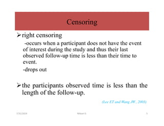
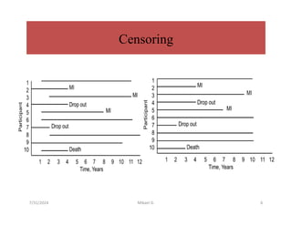
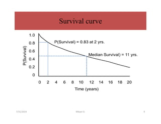
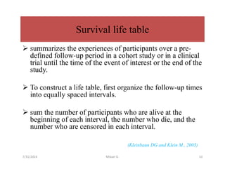
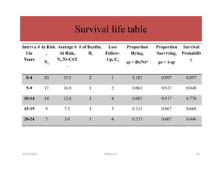
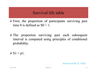
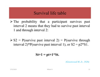
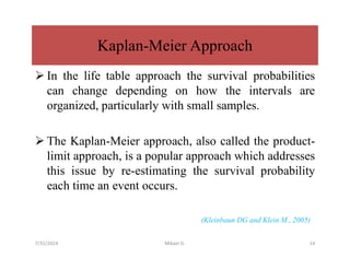
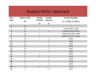
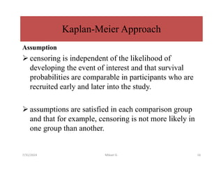
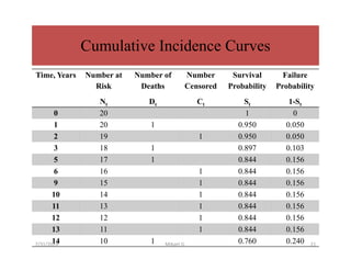
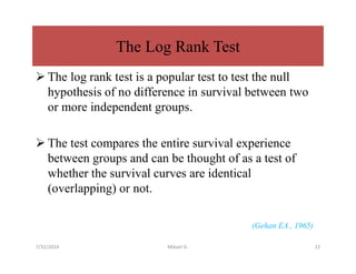
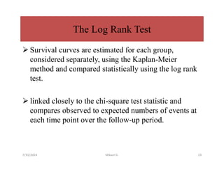
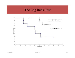
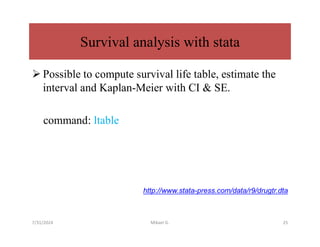
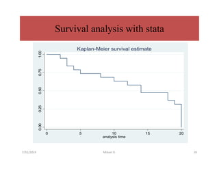
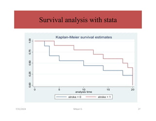
Survival life table and Kaplan-Meier estimate
Mikael Girum (MSc)
HAWASSA UNIVERSITY
COLLEGE OF MEDCINE AND HEALTH SCIENCE
SCHOOL OF PUBLIC HEALTH
7/31/2024 Mikael G. 1
Outline
o Survival data characteristics
o Research questions and hypothesis
o Censoring
o Life table method
o Kaplan-Meier estimate
o Log-rank estimate
o Reference
7/31/2024 Mikael G. 2
Survival data characteristics
 to analyze a "time to event outcome variable"
 "survival" in this context is remaining free of a particular
outcome over time.
 times to event are always positive and their distributions
are often skewed.
 Standard statistical procedures that assume normality of
distributions do not apply.
(Hosmer, DW and Lemeshow, S., 1999)
7/31/2024 Mikael G. 3
 complete data is not always available on each participant in a
study.
 Varied follow up period, drop out & incomplete follow-up
information.
 True survival time (failure time) is not known because the
study ends or because a participant drops out of the study
before experiencing the event.
 What we know is that the participants survival time is greater
than their last observed follow-up time. These times are called
censored times.
Survival data characteristics
7/31/2024
Mikael G. 4
Censoring
right censoring
-occurs when a participant does not have the event
of interest during the study and thus their last
observed follow-up time is less than their time to
event.
-drops out
the participants observed time is less than the
length of the follow-up.
(Lee ET and Wang JW., 2003)
7/31/2024 Mikael G. 5
Censoring
7/31/2024 Mikael G. 6
Research questions
 What is the probability that a participant survives
with certain time?
 Are there differences in survival between groups
(e.g., between those assigned to a new versus a
standard drug in a clinical trial)?
 How do certain personal, behavioral or clinical
characteristics affect participants' chances of
survival?
7/31/2024 Mikael G. 7
Estimating the Survival Function
 Parametric Vs. non parametric
 nonparametric methods make no assumptions about
how the probability that a person develops the event
changes over time.
- estimate and plot the survival distribution or the survival
curve.
(Hosmer, DW and Lemeshow, S., 1999)
7/31/2024 Mikael G. 8
Survival curve
7/31/2024 Mikael G. 9
Survival life table
 summarizes the experiences of participants over a pre-
defined follow-up period in a cohort study or in a clinical
trial until the time of the event of interest or the end of the
study.
 To construct a life table, first organize the follow-up times
into equally spaced intervals.
 sum the number of participants who are alive at the
beginning of each interval, the number who die, and the
number who are censored in each interval.
(Kleinbaun DG and Klein M., 2005)
7/31/2024 Mikael G. 10
Interva
l in
Years
# At Risk
,
Nt
Average #
At Risk,
Nt*Nt-Ct/2
.
# of Deaths,
Dt
Lost
Follow-
Up, Ct
Proportion
Dying,
qt = Dt/Nt*
Proportion
Surviving,
pt = 1-qt
Survival
Probabilit
y
0-4 20 19.5 2 1 0.103 0.897 0.897
5-9 17 16.0 1 2 0.063 0.937 0.840
10-14 14 12.0 1 4 0.083 0.917 0.770
15-19 9 7.5 1 3 0.133 0.867 0.668
20-24 5 3.0 1 4 0.333 0.667 0.446
Survival life table
7/31/2024 Mikael G. 11
 First, the proportion of participants surviving past
time 0 is defined as S0 = 1.
 The proportion surviving past each subsequent
interval is computed using principles of conditional
probability.
 S1 = p1.
(Greenwood M, Jr., 1926)
Survival life table
7/31/2024 Mikael G. 12
 The probability that a participant survives past
interval 2 means that they had to survive past interval
1 and through interval 2:
 S2 = P(survive past interval 2) = P(survive through
interval 2)*P(survive past interval 1), or S2 = p2*S1.
St+1 = pt+1*St.
(Greenwood M, Jr., 1926)
Survival life table
7/31/2024 Mikael G. 13
Kaplan-Meier Approach
 In the life table approach the survival probabilities
can change depending on how the intervals are
organized, particularly with small samples.
 The Kaplan-Meier approach, also called the product-
limit approach, is a popular approach which addresses
this issue by re-estimating the survival probability
each time an event occurs.
(Kleinbaun DG and Klein M., 2005)
7/31/2024 Mikael G. 14
Time,
Years
Number at Risk
Nt
Number
of Deaths
Dt
Number
Censored
Ct
Survival Probability
St+1 = St*((Nt+1-Dt+1)/Nt+1)
0 20 1
1 20 1 1*((20-1)/20) = 0.950
2 19 1 0.950*((19-0)/19)=0.950
3 18 1 0.950*((18-1)/18) = 0.897
5 17 1 0.897*((17-1)/17) = 0.844
6 16 1 0.844
9 15 1 0.844
10 14 1 0.844
11 13 1 0.844
12 12 1 0.844
13 11 1 0.844
14 10 1 0.760
17 9 1 1 0.676
18 7 1 0.676
19 6 1 0.676
21 5 1 0.676
23 4 1 0.507
24 3 3 0.507
Kaplan-Meier Approach
7/31/2024 Mikael G. 15
Assumption
 censoring is independent of the likelihood of
developing the event of interest and that survival
probabilities are comparable in participants who are
recruited early and later into the study.
 assumptions are satisfied in each comparison group
and that for example, censoring is not more likely in
one group than another.
Kaplan-Meier Approach
7/31/2024 Mikael G. 16
 At Time=0 (baseline, or the start of the study), all
participants are at risk and the survival probability is
1 (or 100%).
St+1 = St*((Nt+1-Dt+1)/Nt+1).
(Kleinbaun DG and Klein M., 2005)
Kaplan-Meier Approach
7/31/2024 Mikael G. 17
Standard Errors and Confidence Interval Estimates of
Survival Probabilities
 These estimates of survival probabilities at specific
times and the median survival time are point
estimates.
 Statistical software computing packages.
 A popular formula to estimate the standard error of
the survival estimates is called Greenwoods formula :
(Greenwood M, Jr., 1926)
7/31/2024 Mikael G. 18
Kaplan-Meier with CI
7/31/2024 Mikael G. 19
Cumulative Incidence Curves
 Cumulative incidence, or cumulative failure
probability, is computed as 1-St and can be computed
easily from the life table using the Kaplan-Meier
approach.
(Greenwood M, Jr., 1926)
7/31/2024 Mikael G. 20
Time, Years Number at
Risk
Nt
Number of
Deaths
Dt
Number
Censored
Ct
Survival
Probability
St
Failure
Probability
1-St
0 20 1 0
1 20 1 0.950 0.050
2 19 1 0.950 0.050
3 18 1 0.897 0.103
5 17 1 0.844 0.156
6 16 1 0.844 0.156
9 15 1 0.844 0.156
10 14 1 0.844 0.156
11 13 1 0.844 0.156
12 12 1 0.844 0.156
13 11 1 0.844 0.156
14 10 1 0.760 0.240
Cumulative Incidence Curves
7/31/2024 Mikael G. 21
The Log Rank Test
 The log rank test is a popular test to test the null
hypothesis of no difference in survival between two
or more independent groups.
 The test compares the entire survival experience
between groups and can be thought of as a test of
whether the survival curves are identical
(overlapping) or not.
(Gehan EA., 1965)
7/31/2024 Mikael G. 22
 Survival curves are estimated for each group,
considered separately, using the Kaplan-Meier
method and compared statistically using the log rank
test.
 linked closely to the chi-square test statistic and
compares observed to expected numbers of events at
each time point over the follow-up period.
The Log Rank Test
7/31/2024 Mikael G. 23
The Log Rank Test
7/31/2024 Mikael G. 24
Survival analysis with stata
 Possible to compute survival life table, estimate the
interval and Kaplan-Meier with CI & SE.
command: ltable
http://www.stata-press.com/data/r9/drugtr.dta
7/31/2024 Mikael G. 25
7/31/2024 Mikael G. 26
0.00
0.25
0.50
0.75
1.00
0 5 10 15 20
analysis time
Kaplan-Meier survival estimate
Survival analysis with stata
7/31/2024 Mikael G. 27
0.00
0.25
0.50
0.75
1.00
0 5 10 15 20
analysis time
stroke = 0 stroke = 1
Kaplan-Meier survival estimates
References
Greenwood M, Jr. The Natural Duration of Cancer. Reports of Public Health and Related Subjects
Vol 33, HMSO, London; 1926.
Gehan EA. A Generalized Wilcoxon Test for Comparing Arbitrarily Singly-Censored Samples.
Biometrika. 1965; 52: 203-223.
Hosmer, DW and Lemeshow, S. Applied Survival Analysis: Regression Modeling of Time to
Event Data. NewYork: John Wiley and Sons; 1999.
http://www.stata-press.com/data/r9/drugtr.dta
Kalbfleisch JD and Prentice RL. The Statistical Analysis of Failure Time Data. 2nd ed. New York:
Wiley, 2002.
Kleinbaun DG and Klein M. Survival Analysis: A Self-Learning Text. New York: Springer
Science + Business Median, Inc., 2005.
Lee ET and Wang JW. Statistical Methods for Survival Data Analysis. 3rd edition. New York:
John Wiley & Sons; 2003.
7/31/2024 Mikael G. 28
7/31/2024 Mikael G. 29

survival analysis and kaplan meier analysis.pdf

  • 1.
    Survival life tableand Kaplan-Meier estimate Mikael Girum (MSc) HAWASSA UNIVERSITY COLLEGE OF MEDCINE AND HEALTH SCIENCE SCHOOL OF PUBLIC HEALTH 7/31/2024 Mikael G. 1
  • 2.
    Outline o Survival datacharacteristics o Research questions and hypothesis o Censoring o Life table method o Kaplan-Meier estimate o Log-rank estimate o Reference 7/31/2024 Mikael G. 2
  • 3.
    Survival data characteristics to analyze a "time to event outcome variable"  "survival" in this context is remaining free of a particular outcome over time.  times to event are always positive and their distributions are often skewed.  Standard statistical procedures that assume normality of distributions do not apply. (Hosmer, DW and Lemeshow, S., 1999) 7/31/2024 Mikael G. 3
  • 4.
     complete datais not always available on each participant in a study.  Varied follow up period, drop out & incomplete follow-up information.  True survival time (failure time) is not known because the study ends or because a participant drops out of the study before experiencing the event.  What we know is that the participants survival time is greater than their last observed follow-up time. These times are called censored times. Survival data characteristics 7/31/2024 Mikael G. 4
  • 5.
    Censoring right censoring -occurs whena participant does not have the event of interest during the study and thus their last observed follow-up time is less than their time to event. -drops out the participants observed time is less than the length of the follow-up. (Lee ET and Wang JW., 2003) 7/31/2024 Mikael G. 5
  • 6.
  • 7.
    Research questions  Whatis the probability that a participant survives with certain time?  Are there differences in survival between groups (e.g., between those assigned to a new versus a standard drug in a clinical trial)?  How do certain personal, behavioral or clinical characteristics affect participants' chances of survival? 7/31/2024 Mikael G. 7
  • 8.
    Estimating the SurvivalFunction  Parametric Vs. non parametric  nonparametric methods make no assumptions about how the probability that a person develops the event changes over time. - estimate and plot the survival distribution or the survival curve. (Hosmer, DW and Lemeshow, S., 1999) 7/31/2024 Mikael G. 8
  • 9.
  • 10.
    Survival life table summarizes the experiences of participants over a pre- defined follow-up period in a cohort study or in a clinical trial until the time of the event of interest or the end of the study.  To construct a life table, first organize the follow-up times into equally spaced intervals.  sum the number of participants who are alive at the beginning of each interval, the number who die, and the number who are censored in each interval. (Kleinbaun DG and Klein M., 2005) 7/31/2024 Mikael G. 10
  • 11.
    Interva l in Years # AtRisk , Nt Average # At Risk, Nt*Nt-Ct/2 . # of Deaths, Dt Lost Follow- Up, Ct Proportion Dying, qt = Dt/Nt* Proportion Surviving, pt = 1-qt Survival Probabilit y 0-4 20 19.5 2 1 0.103 0.897 0.897 5-9 17 16.0 1 2 0.063 0.937 0.840 10-14 14 12.0 1 4 0.083 0.917 0.770 15-19 9 7.5 1 3 0.133 0.867 0.668 20-24 5 3.0 1 4 0.333 0.667 0.446 Survival life table 7/31/2024 Mikael G. 11
  • 12.
     First, theproportion of participants surviving past time 0 is defined as S0 = 1.  The proportion surviving past each subsequent interval is computed using principles of conditional probability.  S1 = p1. (Greenwood M, Jr., 1926) Survival life table 7/31/2024 Mikael G. 12
  • 13.
     The probabilitythat a participant survives past interval 2 means that they had to survive past interval 1 and through interval 2:  S2 = P(survive past interval 2) = P(survive through interval 2)*P(survive past interval 1), or S2 = p2*S1. St+1 = pt+1*St. (Greenwood M, Jr., 1926) Survival life table 7/31/2024 Mikael G. 13
  • 14.
    Kaplan-Meier Approach  Inthe life table approach the survival probabilities can change depending on how the intervals are organized, particularly with small samples.  The Kaplan-Meier approach, also called the product- limit approach, is a popular approach which addresses this issue by re-estimating the survival probability each time an event occurs. (Kleinbaun DG and Klein M., 2005) 7/31/2024 Mikael G. 14
  • 15.
    Time, Years Number at Risk Nt Number ofDeaths Dt Number Censored Ct Survival Probability St+1 = St*((Nt+1-Dt+1)/Nt+1) 0 20 1 1 20 1 1*((20-1)/20) = 0.950 2 19 1 0.950*((19-0)/19)=0.950 3 18 1 0.950*((18-1)/18) = 0.897 5 17 1 0.897*((17-1)/17) = 0.844 6 16 1 0.844 9 15 1 0.844 10 14 1 0.844 11 13 1 0.844 12 12 1 0.844 13 11 1 0.844 14 10 1 0.760 17 9 1 1 0.676 18 7 1 0.676 19 6 1 0.676 21 5 1 0.676 23 4 1 0.507 24 3 3 0.507 Kaplan-Meier Approach 7/31/2024 Mikael G. 15
  • 16.
    Assumption  censoring isindependent of the likelihood of developing the event of interest and that survival probabilities are comparable in participants who are recruited early and later into the study.  assumptions are satisfied in each comparison group and that for example, censoring is not more likely in one group than another. Kaplan-Meier Approach 7/31/2024 Mikael G. 16
  • 17.
     At Time=0(baseline, or the start of the study), all participants are at risk and the survival probability is 1 (or 100%). St+1 = St*((Nt+1-Dt+1)/Nt+1). (Kleinbaun DG and Klein M., 2005) Kaplan-Meier Approach 7/31/2024 Mikael G. 17
  • 18.
    Standard Errors andConfidence Interval Estimates of Survival Probabilities  These estimates of survival probabilities at specific times and the median survival time are point estimates.  Statistical software computing packages.  A popular formula to estimate the standard error of the survival estimates is called Greenwoods formula : (Greenwood M, Jr., 1926) 7/31/2024 Mikael G. 18
  • 19.
  • 20.
    Cumulative Incidence Curves Cumulative incidence, or cumulative failure probability, is computed as 1-St and can be computed easily from the life table using the Kaplan-Meier approach. (Greenwood M, Jr., 1926) 7/31/2024 Mikael G. 20
  • 21.
    Time, Years Numberat Risk Nt Number of Deaths Dt Number Censored Ct Survival Probability St Failure Probability 1-St 0 20 1 0 1 20 1 0.950 0.050 2 19 1 0.950 0.050 3 18 1 0.897 0.103 5 17 1 0.844 0.156 6 16 1 0.844 0.156 9 15 1 0.844 0.156 10 14 1 0.844 0.156 11 13 1 0.844 0.156 12 12 1 0.844 0.156 13 11 1 0.844 0.156 14 10 1 0.760 0.240 Cumulative Incidence Curves 7/31/2024 Mikael G. 21
  • 22.
    The Log RankTest  The log rank test is a popular test to test the null hypothesis of no difference in survival between two or more independent groups.  The test compares the entire survival experience between groups and can be thought of as a test of whether the survival curves are identical (overlapping) or not. (Gehan EA., 1965) 7/31/2024 Mikael G. 22
  • 23.
     Survival curvesare estimated for each group, considered separately, using the Kaplan-Meier method and compared statistically using the log rank test.  linked closely to the chi-square test statistic and compares observed to expected numbers of events at each time point over the follow-up period. The Log Rank Test 7/31/2024 Mikael G. 23
  • 24.
    The Log RankTest 7/31/2024 Mikael G. 24
  • 25.
    Survival analysis withstata  Possible to compute survival life table, estimate the interval and Kaplan-Meier with CI & SE. command: ltable http://www.stata-press.com/data/r9/drugtr.dta 7/31/2024 Mikael G. 25
  • 26.
    7/31/2024 Mikael G.26 0.00 0.25 0.50 0.75 1.00 0 5 10 15 20 analysis time Kaplan-Meier survival estimate Survival analysis with stata
  • 27.
    7/31/2024 Mikael G.27 0.00 0.25 0.50 0.75 1.00 0 5 10 15 20 analysis time stroke = 0 stroke = 1 Kaplan-Meier survival estimates
  • 28.
    References Greenwood M, Jr.The Natural Duration of Cancer. Reports of Public Health and Related Subjects Vol 33, HMSO, London; 1926. Gehan EA. A Generalized Wilcoxon Test for Comparing Arbitrarily Singly-Censored Samples. Biometrika. 1965; 52: 203-223. Hosmer, DW and Lemeshow, S. Applied Survival Analysis: Regression Modeling of Time to Event Data. NewYork: John Wiley and Sons; 1999. http://www.stata-press.com/data/r9/drugtr.dta Kalbfleisch JD and Prentice RL. The Statistical Analysis of Failure Time Data. 2nd ed. New York: Wiley, 2002. Kleinbaun DG and Klein M. Survival Analysis: A Self-Learning Text. New York: Springer Science + Business Median, Inc., 2005. Lee ET and Wang JW. Statistical Methods for Survival Data Analysis. 3rd edition. New York: John Wiley & Sons; 2003. 7/31/2024 Mikael G. 28
  • 29.