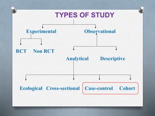
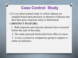
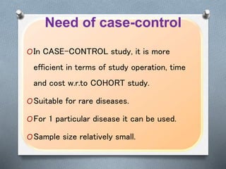
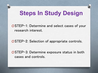
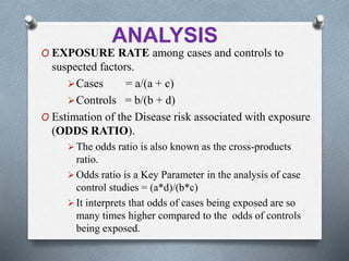
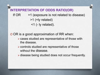
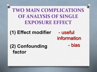
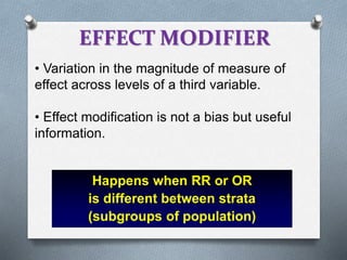
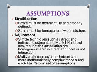
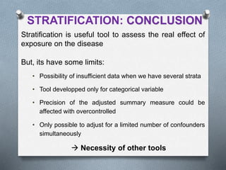
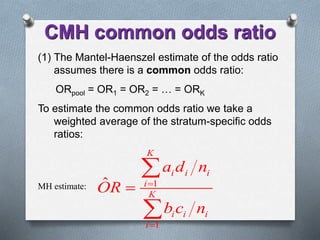
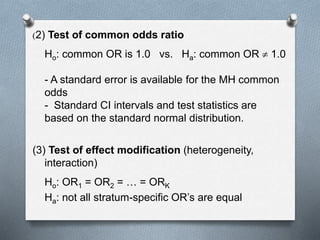
This document discusses case-control studies and their design and analysis. It begins by defining case-control studies as observational studies where subjects are sampled based on disease presence or absence and their prior exposure is then determined. It describes key features, need, steps in design including case and control selection. It then covers statistical analysis including odds ratios to measure risk associated with exposure and interpretations. It discusses effect modification and confounding, and analytical tools like stratification and multivariate modeling to control for confounding.
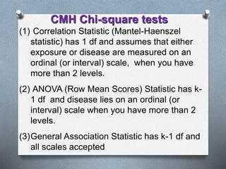
Study designs, Epidemiological study design, Types of studiesDr Lipilekha Patnaik
Study design, Epidemiological study designA study design is a specific plan or protocol
for conducting the study, which allows the investigator to translate the conceptual hypothesis into an operational one.
The ppt is a short description about how to ascertain the validity, ie; sensitivity and specificity of a screening test as well as their predictive powers. you can also find the technique to ascertain the best possible screening test through the help of an ROC curve...
In this presentation , we explain what is study design ,
why we need study design,
types of study design,
case control study design,
what is sample and how to estimate sample size
Excelsior College PBH 321 Page 1 CASE-CONTROL STU.docxgitagrimston
Excelsior College PBH 321
Page 1
CASE-CONTROL STUD IES
A case-control study is an observational design that involves studying a population in which cases of disease
are identified and enrolled, and a sample of the population that produced the cases is identified and enrolled
(controls). Exposures are determined for individuals in both groups.
Let’s say that we want to test the hypothesis that pesticide exposure increases the risk of breast cancer.
Consider a hypothetical prospective cohort study of 89,949 women aged 34-59; 1,439 breast cancer cases
were identified over 8 years of follow-up. Blood was drawn on all 89,949 at beginning of follow-up and
samples were frozen. The exposure was defined as the level of pesticides (e.g. DDE) in blood, characterized as
high or low. We compare women with high or low exposures to see if they got breast cancer or not by the end
of follow-up.
Breast Cancer
Yes No Total
DDE
exposure High 360 13,276 13,636
Relative Risk = RR = (360/13,636) / (1,079/76,313) = 1.9
Low 1,079 75,234 76,313
Women with high pesticide levels in the blood have 1.9
times the risk of developing breast cancer after 8 years
than women with low levels
Total 1,439 88,510 89,949
Conducting this study presents a practical problem: quantifying pesticide levels in the blood is very expensive -
-it's not feasible to analyze all 89,949 blood samples (this would cost many thousands of dollars).
To be efficient, we could instead analyze blood on all breast cancer cases (N=1,439) but take only a sample of
the women who did not get breast cancer, say two times as many cases (N=2,878) (controls). This is a case-
control study! Specifically, because we sampled cases and controls from within a complete cohort, we refer to
this as a nested case-control study.
Breast Cancer
Cases Controls
DDE
exposure
High 360 432
Low 1,079 2,446
Total 1,439 2,878
Excelsior College PBH 321
Page 2
Timing and Set Up of a Case-Control Study
Cases
When identifying cases, the criteria for the case definition should lead to accurate classification of disease.
This means the investigator must have efficient and accurate sources to identify cases, such as existing disease
registries or hospitals.
In our standard 2 x 2 table, the number of cases gives you the numerators of the rates of disease in exposed
and unexposed groups being compared.
Disease
Yes
(cases)
No
(controls)
Total
Exposure Yes a ? ? Rate of disease in exposed: a/?
No c ? ?
Rate of disease in
unexposed: c/?
Total a+c ? ?
What is missing? The denominators! If this were a cohort study, you would have the total population (if you
were calculating cumulative incidence) or total person-years (if you were calculating incidence rates) for both
the exposed and non-exposed groups, which would provide the c ...
Richard's aventures in two entangled wonderlandsRichard Gill
Since the loophole-free Bell experiments of 2020 and the Nobel prizes in physics of 2022, critics of Bell's work have retreated to the fortress of super-determinism. Now, super-determinism is a derogatory word - it just means "determinism". Palmer, Hance and Hossenfelder argue that quantum mechanics and determinism are not incompatible, using a sophisticated mathematical construction based on a subtle thinning of allowed states and measurements in quantum mechanics, such that what is left appears to make Bell's argument fail, without altering the empirical predictions of quantum mechanics. I think however that it is a smoke screen, and the slogan "lost in math" comes to my mind. I will discuss some other recent disproofs of Bell's theorem using the language of causality based on causal graphs. Causal thinking is also central to law and justice. I will mention surprising connections to my work on serial killer nurse cases, in particular the Dutch case of Lucia de Berk and the current UK case of Lucy Letby.
This pdf is about the Schizophrenia.
For more details visit on YouTube; @SELF-EXPLANATORY;
https://www.youtube.com/channel/UCAiarMZDNhe1A3Rnpr_WkzA/videos
Thanks...!
Professional air quality monitoring systems provide immediate, on-site data for analysis, compliance, and decision-making.
Monitor common gases, weather parameters, particulates.
A brief information about the SCOP protein database used in bioinformatics.
The Structural Classification of Proteins (SCOP) database is a comprehensive and authoritative resource for the structural and evolutionary relationships of proteins. It provides a detailed and curated classification of protein structures, grouping them into families, superfamilies, and folds based on their structural and sequence similarities.
Slide 1: Title Slide
Extrachromosomal Inheritance
Slide 2: Introduction to Extrachromosomal Inheritance
Definition: Extrachromosomal inheritance refers to the transmission of genetic material that is not found within the nucleus.
Key Components: Involves genes located in mitochondria, chloroplasts, and plasmids.
Slide 3: Mitochondrial Inheritance
Mitochondria: Organelles responsible for energy production.
Mitochondrial DNA (mtDNA): Circular DNA molecule found in mitochondria.
Inheritance Pattern: Maternally inherited, meaning it is passed from mothers to all their offspring.
Diseases: Examples include Leber’s hereditary optic neuropathy (LHON) and mitochondrial myopathy.
Slide 4: Chloroplast Inheritance
Chloroplasts: Organelles responsible for photosynthesis in plants.
Chloroplast DNA (cpDNA): Circular DNA molecule found in chloroplasts.
Inheritance Pattern: Often maternally inherited in most plants, but can vary in some species.
Examples: Variegation in plants, where leaf color patterns are determined by chloroplast DNA.
Slide 5: Plasmid Inheritance
Plasmids: Small, circular DNA molecules found in bacteria and some eukaryotes.
Features: Can carry antibiotic resistance genes and can be transferred between cells through processes like conjugation.
Significance: Important in biotechnology for gene cloning and genetic engineering.
Slide 6: Mechanisms of Extrachromosomal Inheritance
Non-Mendelian Patterns: Do not follow Mendel’s laws of inheritance.
Cytoplasmic Segregation: During cell division, organelles like mitochondria and chloroplasts are randomly distributed to daughter cells.
Heteroplasmy: Presence of more than one type of organellar genome within a cell, leading to variation in expression.
Slide 7: Examples of Extrachromosomal Inheritance
Four O’clock Plant (Mirabilis jalapa): Shows variegated leaves due to different cpDNA in leaf cells.
Petite Mutants in Yeast: Result from mutations in mitochondrial DNA affecting respiration.
Slide 8: Importance of Extrachromosomal Inheritance
Evolution: Provides insight into the evolution of eukaryotic cells.
Medicine: Understanding mitochondrial inheritance helps in diagnosing and treating mitochondrial diseases.
Agriculture: Chloroplast inheritance can be used in plant breeding and genetic modification.
Slide 9: Recent Research and Advances
Gene Editing: Techniques like CRISPR-Cas9 are being used to edit mitochondrial and chloroplast DNA.
Therapies: Development of mitochondrial replacement therapy (MRT) for preventing mitochondrial diseases.
Slide 10: Conclusion
Summary: Extrachromosomal inheritance involves the transmission of genetic material outside the nucleus and plays a crucial role in genetics, medicine, and biotechnology.
Future Directions: Continued research and technological advancements hold promise for new treatments and applications.
Slide 11: Questions and Discussion
Invite Audience: Open the floor for any questions or further discussion on the topic.
Seminar of U.V. Spectroscopy by SAMIR PANDASAMIR PANDA
Spectroscopy is a branch of science dealing the study of interaction of electromagnetic radiation with matter.
Ultraviolet-visible spectroscopy refers to absorption spectroscopy or reflect spectroscopy in the UV-VIS spectral region.
Ultraviolet-visible spectroscopy is an analytical method that can measure the amount of light received by the analyte.
2. TYPES OF STUDY
Experimental Observational
RCT Non RCT
Analytical Descriptive
Ecological Cross-sectional Case-control Cohort
3. Case Control Study
O It is an observational study in which subjects are
sampled based upon presence or absence of disease and
then their prior exposure status is determined.
O DISTINCT FEATURE:
1. Both exposure and outcome (disease) have occurred
before the start of the study.
2. The study proceeds backwards from effect to cause.
3. It uses a control or comparison group to support or
refute an inference.
4. Need of case-control
OIn CASE-CONTROL study, it is more
efficient in terms of study operation, time
and cost w.r.to COHORT study.
OSuitable for rare diseases.
OFor 1 particular disease it can be used.
OSample size relatively small.
5. Steps In Study Design
OSTEP-1: Determine and select cases of your
research interest.
OSTEP-2: Selection of appropriate controls.
OSTEP-3: Determine exposure status in both
cases and controls.
6. Cases Selection
O Study begins with cases, i.e. the patients in whom the
disease has already occurred.
O Patients with the disease in question (cases) were
enquired for all the details of their exposure to the
suspected cause.
O The new cases, which are similar clinically,
histologically, pathologically and in their duration of
exposure (stage) will be chosen to avoid any error and
for better comparison.
Sources of Cases
Hospitals.
General population
7. Who will be controls?
O Control ≠ non-case
O Controls are also at risk of the disease in his(her)
future.
O “Controls” are expected to be a representative sample
of the catchment population from which the case arise.
O For e.g. in a case-control study of gastric cancer, a
person who has received the Gastrectomy cannot be a
control since he never develop gastric cancer .
Sources of controls:
Hospital controls
General population
Relatives/Neighborhood
9. Statistical analysis
“Matched” vs. “Unmatched”
studies
The procedures for analyzing the results of
case-control studies differ depending on
whether the cases and controls are
matched or unmatched.
Matched Unmatched
・McNemar’s test ・Chi-square test
・Conditional logistic ・Unconditional logistic
regression analysis regression analysis
10. ANALYSIS
O EXPOSURE RATE among cases and controls to
suspected factors.
Cases = a/(a + c)
Controls = b/(b + d)
O Estimation of the Disease risk associated with exposure
(ODDS RATIO).
The odds ratio is also known as the cross-products
ratio.
Odds ratio is a Key Parameter in the analysis of case
control studies = (a*d)/(b*c)
It interprets that odds of cases being exposed are so
many times higher compared to the odds of controls
being exposed.
11. INTERPRETATION OF ODDS RATIO(OR)
If OR =1 (exposure is not related to disease)
>1 (+ly related)
<1 (- ly related).
O OR is a good approximation of RR when:
cases studied are representative of those with
the disease.
controls studied are representative of those
without the disease.
disease being studied does not occur frequently.
12. TWO MAIN COMPLICATIONS
OF ANALYSIS OF SINGLE
EXPOSURE EFFECT
(1) Effect modifier
(2) Confounding
factor
- useful
information
- bias
13. EFFECT MODIFIER
• Variation in the magnitude of measure of
effect across levels of a third variable.
• Effect modification is not a bias but useful
information.
Happens when RR or OR
is different between strata
(subgroups of population)
14. Continue….
• To study interaction between risk
factors.
• To identify a subgroup with a lower or
higher risk.
• To target public health action.
• Better understand of the disease:
biological mechanism.
15. To identify a subgroup with a
lower or higher risk
• Example 1 : Influenza :
O Important complications for
old people, for person with
cardiac and pulmonary
disease or diabetes…
O The risk of complication is
more higher for these
categories of people.
O Age and comorbidity are
effect modifiers for
influenza.
To target public health action
• Example 1 : Influenza
• Vaccination is
recommanded for :
Old person,
Person with cardiac and
pulmonary disease .
Diabetes …
EFFECT MODIFICATION : EXAMPLE
17. OShould be prevented or Needs to be
controlled for.
ODistortion of measure of effect because of
a third factor.
OStratification and Multivariate modeling are
the analytic tools used to control for
confounding.
OStratification allows for assessment of
confounding and effect modification.
OMultivariate analyses are used to carry out
statistical adjustment.
Continue….
18. ASSUMPTIONS
Stratification
O Strata must be meaningfully and properly
defined.
O Strata must be homogenous within stratum.
Adjustment
O Simple techniques such as direct and
indirect adjustment and Mantel-Haenszel
assume that the association are
homogenous across strata and there is not
interaction
O Multivariate regression techniques are
more mathematically complex models and
each has it’s own set of assumptions
19. • Positive confounding
- positively or negatively related to both
the disease and exposure
• Negative confounding
- positively related to disease but is
negatively related to exposure or the
reverse
20. Confounding: example
Drinker
Non-drinker
100 200
Lung cancer No lung
cancer
50 50
50 150
50% of cases are drinkers, but only 25% of
controls are drinkers.
Therefore, it appears that drinking is strongly
associated with lung cancer.
21. CONFOUNDING: EXAMPLE
Drinker
Non-drinker
Lung
cancer
No lung
cancer
45 15
30 10
Drinker
Non-drinker
Lung cancer No lung
cancer
5 35
20 140
Smoker
Non-smoker
Among smokers,
45/75=60% of lung
cancer cases drink
and
15/25=60% of
controls drink.
Among non-smokers
5/25=20% of lung
cancer cases drink
and
35/175=20% of
controls drink.
75
25
25
175
23. STRATIFICATION AND
MULTIVARIATE MODELING
OStratification and Multivariate modeling are
the analytic tools used to control for
confounding
OStratification allows for assessment of
confounding and effect modification
OMultivariate analyses are used to carry out
statistical adjustment
24. GENERAL FRAMEWORK FOR
STRATIFICATION
In the study design phase:
• Decide which variables to control for
In the implementation phase:
• Measure the confounders or other variables
needed to block path
In the analytical phase:
• Assess clinical, statistical and practical
consideration
25. STRATIFICATION: Principle
Principle :
O Create strata according to categories of
the third variable
O Perfom analysis inside these strata
O Conclude about the studied relation
inside the strata
O Forming «adjusted summary
estimate»: concept of weighted average
O Assumption: weak variability in the strata
26. TO PERFORM A STRATIFIED ANALYSIS,WE HAVE 6
STEPS:
1. Carry out simple analysis to test the association between the
exposure and the disease and to Identify potential
confounder
2. Categorize the confounder and divide the sample in
strata, according to the number of categories of the
confounder
3. Carry out simple analysis to test the association between
the exposure and the disease in each stratum
4. Test the presence or absence of effect modification
between the variables
5. If appropriate, check for confounding and calculate a point
estimate of overall effect (weighted average measure)
6. If appropriate, carry out and interpret an overall test for
association
27. STRATIFICATION: CONCLUSION
Stratification is useful tool to assess the real effect of
exposure on the disease
But, its have some limits:
• Possibility of insufficient data when we have several strata
• Tool developped only for categorical variable
• Precision of the adjusted summary measure could be
affected with overcontrolled
• Only possible to adjust for a limited number of confounders
simultaneously
Necessity of other tools
28. MULTIVARIATE ANALYSIS
Definition: A technique that takes into account
a number of variables simultaneously.
• Involves construction of a mathematical
model that efficiently describes the
association between exposure and disease,
as well as other variables that may confound
or modify the effect of exposure.
Examples:
Multiple linear regression model
Logistic regression model
29. MULTIPLE LINEAR REGRESSION MODEL:
Y = a + b1X1 + b2X2 + …bnXn
Where:
n = the number of independent variables (IVs)
(e.g. Exposure(s) and confounders)
X1 … Xn = individual’s set of values for the Ivs
b1 … bn = respective coefficients for the IVs
30. LOGISTIC REGRESSION MODEL:
ln [Y / (1-Y)] = a + b1X1 + b2X2 + …bnXn
Where:
Y = probability of disease
n = the number of independent variables
(IVs)
(e.g. exposure(s) and confounders)
X1 … Xn = individual’s set of values for the
IVs
b1 … bn = respective coefficients for the IVs
32. Assess association between disease and
exposure after controlling for one or more
confounding variables.
ai
ci
bi
di
(ai + ci) (bi + di)
(ai + bi)
(ci + di)
ni
D
D
E E
where i = 1,2,…,K is the number of
strata
Mantel Haenszel
Methods-Notations
33. (1) Correlation Statistic (Mantel-Haenszel
statistic) has 1 df and assumes that either
exposure or disease are measured on an
ordinal (or interval) scale, when you have
more than 2 levels.
(2) ANOVA (Row Mean Scores) Statistic has k-
1 df and disease lies on an ordinal (or
interval) scale when you have more than 2
levels.
(3)General Association Statistic has k-1 df and
all scales accepted
CMH Chi-square tests
34. (1) The Mantel-Haenszel estimate of the odds ratio
assumes there is a common odds ratio:
ORpool = OR1 = OR2 = … = ORK
To estimate the common odds ratio we take a
weighted average of the stratum-specific odds
ratios:
MH estimate: 1
1
ˆ
K
i i i
i
K
i i i
i
a d n
OR
b c n
CMH common odds ratio
35. (2) Test of common odds ratio
Ho: common OR is 1.0 vs. Ha: common OR 1.0
- A standard error is available for the MH common
odds
- Standard CI intervals and test statistics are
based on the standard normal distribution.
(3) Test of effect modification (heterogeneity,
interaction)
Ho: OR1 = OR2 = … = ORK
Ha: not all stratum-specific OR’s are equal
36. 36
Computing Cochran-Mantel-
Haenszel Statistics for a Stratified
Table
OThe data set Migraine contains
hypothetical data for a clinical trial of
migraine treatment. Subjects of both
genders receive either a new drug
therapy or a placebo. Assess the effect of
new drug adjusting for gender.
37. 37
Example - Migraine
Response
Treatment Better Same Total
Active 28 27 55
Placebo 12 39 51
Total 40 66 106
Pearson Chi-squares test p = 0.0037
But after stratify by sex, it will be different for male vs female.
38. 38
Male Response
Treatment Better Same Total
Active 12 16 28
p = 0.2205
Placebo 7 19 26
Total 19 35 54
Female Response
Treatment Better Same Total
Active 16 11 27
p = 0.0039
Placebo 5 20 25
Total 21 31 52
39. 39
Comments
O The significant p-value (0.004) indicates that the
association between treatment and response
remains strong after adjusting for gender
O The probability of migraine improvement with the
new drug is just over two times the probability of
improvement with the placebo.
O The large p-value for the Breslow-Day test (0.2218)
indicates no significant gender difference in the
odds ratios.
Editor's Notes
refute;
prove (a statement or theory) to be wrong or false; disprove.
A gastrectomy is a medical procedure where all or part of the stomach is surgically removed. There are four types of gastrectomy: total gastrectomy – the whole stomach is removed. partial gastrectomy – the lower part of the stomach is removed
In medicine, comorbidity is the presence of one or more additional disorders (or diseases) co-occurring with a primary disease or disorder; or the effect of such additional disorders or diseases. The additional disorder may also be a behavioral or mental disorder.