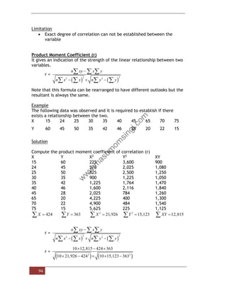
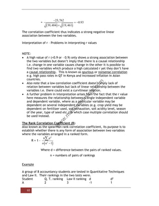
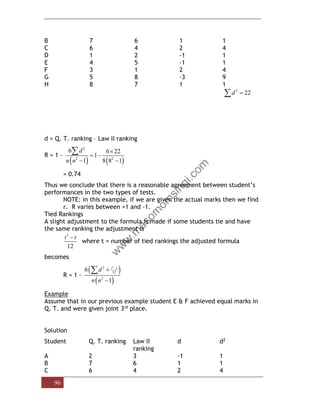
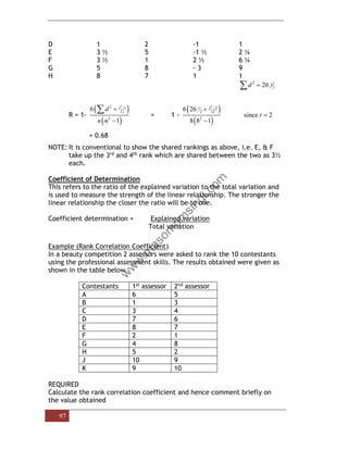
SlideShare a Scribd company logo
1 of 22
Download to read offline
87
Moment coefficient of Kurtosis
M4
S4
Example
Find the moment coefficient of the following distribution
X f
12 1
14 4
16 6
18 10
20 7
22 2
X F xf (x-m) (x-m)2 (x-m)2f (x-m)4f
12 1 12 -5.6 31.36 31.36 983.45
14 4 56 -3.6 12.96 51.84 671.85
16 6 96 -1.6 2.56 15.36 39.32
18 10 180 .4 0.16 1.60 0.256
20 7 140 2.4 5.76 40.32 232.24
22 2 44 4.4 19.36 38.72 749.62
30 528 179.20 2,676.74
M =
528
30
= 17.6
σ2 =
179.20
30
= 5.973
σ4 = 35.677
M4 =
( )
4
x m f
f
−


=
2,676.74
30
= 89.22
Moment coefficient of Kurtosis =
89.22
35.677
= 2.5
Note Coefficient of kurtosis can also be found using the method of assumed
mean.
CHAPTER FIVE
CORRELATION AND REGRESSION
88
Specific Objectives
At the end of the topic the trainee should be able to:
➢ Draw the scatter diagram;
➢ Differentiate between the various forms of correlation;
➢ Determine the correlation coefficient and interpret;
➢ Determine the coefficient of determination and interpret;
➢ Apply the linear regression models.
Introduction
When the relationship is of a quantitative nature, the appropriate
statistical tool for discovering and measuring the relationship and
expressing it in a brief formula is known as a correlation. This is an
important statistical concept which refers to interrelationship or
association between variables. The purpose of studying correlation is for
one to be able to establish a relationship, plan and control the inputs
(independent variables) and the output (dependent variables).
In business one may be interested to establish whether there exists a
relationship between the
i. Amount of fertilizer applied on a given farm and the resulting
harvest
ii. Amount of experience one has and the corresponding
performance
iii. Amount of money spent on advertisement and the expected
incomes after sale of the goods/service
There are two methods that measure the degree of correlation between
two variables these are denoted by R and r.
(a) Coefficient of correlation denoted by r, this provides a measure of
the strength of association between two variables one the dependent
variable the other the independent variable r can range between +1
and – 1 for perfect positive correlation and perfect negative
correlation respectively with zero indicating no relation i.e. for
perfect positive correlation y increase linearly with x increment.
(b) Rank correlation coefficient denoted by R is used to measure
association between two sets of ranked or ordered data. R can also
vary from +1, perfect positive rank correlation and -1 perfect
negative rank correlation where O or any number near zero
representing no correlation.
89
Significance of the study of correlation
➢ Most of the variation shows some kind of relationship between price
and supply income and expenditure. With the help of correlation
analysis the degree of relationship existing between the variable can
be measured.
➢ The value of one variable can be estimated once it has been known
that they closely related. It can be done with the help of regression
analysis.
➢ It contributes to the economic behavior, aids in locating the critically
important variable on which other depend.
➢ Nature has been found to be multiplying of interrelated force.
➢ It helps in determining the degree of relationship between two or
more variable.
Types of correlation
• Positive and negative correlation
• Simple, partial and multiple
• Linear and non linear.
Positive and negative correlation
If both the variable is varying in the same direction i.e. if one variable is
increasing the other on an average is also increasing or if one variable is
decreasing the other on an average is also decreasing. Correlation is said to
be positive. On the other hand if they are varying in the opposite directions
i.e. as one variable is increasing the other is decreasing or vice versa,
correlation is said to be negative.
Positive correlation negative correlation
X T X T
10 15 20 40
12 20 30 30
15 22 40 22
18 25 60 15
20 37 80 16
Simple partial and multiple correlations
The distribution between simple, partial and multiple correlations are
based upon the number of variable studied.
When only two variables are studied it is a problem of simple correlation.
When three or more variables are studied it is a problem of either
Multiple or partial correlation.
In multiple correlations three or more variables are studied simultaneously.
90
Linear and non linear correlation
The distinction between linear and non linear correlation is based upon the
constancy of the ratio of change between the variables. If the amount of
change in one variable tends to bear constant ratio to the amount of
change in the other variable then the correlation is said to be linear. If such
variable are plotted on a graph paper, all the plotted points would fall on a
straight line. Correlation would be non linear or curvilinear, If the amount
of change in one variable does not bear constant ratio to the amount of
change in the other variable.
Scatter diagram
The simplest device for studying correlation in two variables is a special
type of dot chart called dotogram or scatter diagram.
A scatter graph is a graph which comprises of points which have been
plotted but are not joined by line segments
The pattern of the points will definitely reveal the types of relationship
existing between variables
The following sketch graphs will greatly assist in the interpretation of
scatter graphs.
Perfect positive correlation
y
Dependant variable x
x
x
x
x
x
x
x
Independent variable
NB: For the above pattern, it is referred to as perfect because the points
may easily be represented by a single line graph e.g. when measuring
relationship between volumes of sales and profits in a company, the more
the company sales the higher the profits.
91
Perfect negative correlation
y x
Quantity sold x
X
x
x
x
x
x
x
10 20 X
Price
This example considers volume of sale in relation to the price, the cheaper
the goods the bigger the sale.
High positive correlation
y
Dependant variable xx
xx
x
x
xx
xx
xx
xx
x
xxx
x
x
Independent variable
High negative correlation
y
Quantity sold x
92
x
xx
x
xx
x
x
x
x
xx
x
price
No correlation
y
600 x x x x x
x x x
400 x x x x x
x x x x
200 x x x x x
x x x x
0
10 20 30 40 50 x
h) Spurious Correlations
93
in some rare situations when plotting the data for x and y we may have
a group showing either positive correlation or –ve correlation but when
you analyze the data for x and y in normal life there may be no
convincing evidence that there is such a relationship. This implies
therefore that the relationship only exists in theory and hence it is
referred to as spurious or non sense e.g. when high pass rates of student
show high relation with increased accidents.
Correlation coefficient
These are numerical measures of the correlations existing between the
dependent and the independent variables. These are better measures of
correlation than scatter graphs (diagrams).The range for correlation
coefficients lies between +ve 1 and –ve 1. A correlation coefficient of +1
implies that there is perfect positive correlation. A value of –ve shows
that there is perfect negative correlation. A value of 0 implies no
correlation at all.
The following chart will be found useful in interpreting correlation
coefficients.
__ 1.0} Perfect +ve correlation
} High positive correlation
__ 0.5 }
} Low positive correlation
__0 }
} Low negative correlation
__-0.5}
} High negative correlation
__-1.0} Perfect –ve correlation
There are usually two types of correlation coefficients normally used
namely;-
Merits of scatter diagram
• It is simple and non mathematical method of studying correlation
between the variables.
• It is not influenced by the size of extreme values whereas most of
the mathematical methods of findings correlation are influenced by
extreme values.
94
Limitation
• Exact degree of correlation can not be established between the
variable
Product Moment Coefficient (r)
It gives an indication of the strength of the linear relationship between two
variables.
r =
( ) ( )
2 2
2 2
n xy x y
n x x n y y
−
−  −
  
   
Note that this formula can be rearranged to have different outlooks but the
resultant is always the same.
Example
The following data was observed and it is required to establish if there
exists a relationship between the two.
X 15 24 25 30 35 40 45 65 70 75
Y 60 45 50 35 42 46 28 20 22 15
Solution
Compute the product moment coefficient of correlation (r)
X Y X2 Y2 XY
15 60 225 3,600 900
24 45 576 2,025 1,080
25 50 625 2,500 1,250
30 35 900 1,225 1,050
35 42 1,225 1,764 1,470
40 46 1,600 2,116 1,840
45 28 2,025 784 1,260
65 20 4,225 400 1,300
70 22 4,900 484 1,540
75 15 5,625 225 1,125
424
X =
 363
Y =
 2
21,926
X =
 2
15,123
Y =
 12,815
XY =

r =
( ) ( )
2 2
2 2
n xy x y
n x x n y y
−
−  −
  
   
r =
( ) ( )
2 2
10 12,815 424 363
10 21,926 424 10 15,123 363
 − 
 −   −
95
=
( ) ( )
25,762
0.93
39,484 19,461
−
= −

The correlation coefficient thus indicates a strong negative linear
association between the two variables.
Interpretation of r – Problems in interpreting r values
NOTE:
• A high value of r (+0.9 or – 0.9) only shows a strong association between
the two variables but doesn’t imply that there is a causal relationship
i.e. change in one variable causes change in the other it is possible to
find two variables which produce a high calculated r yet they don’t have
a causal relationship. This is known as spurious or nonsense correlation
e.g. high pass rates in QT in Kenya and increased inflation in Asian
countries.
• Also note that a low correlation coefficient doesn’t imply lack of
relation between variables but lack of linear relationship between the
variables i.e. there could exist a curvilinear relation.
• A further problem in interpretation arises from the fact that the r value
here measures the relationship between a single independent variable
and dependent variable, where as a particular variable may be
dependent on several independent variables (e.g. crop yield may be
dependent on fertilizer used, soil exhaustion, soil acidity level, season
of the year, type of seed etc.) in which case multiple correlation should
be used instead.
The Rank Correlation Coefficient (R)
Also known as the spearman rank correlation coefficient, its purpose is to
establish whether there is any form of association between two variables
where the variables arranged in a ranked form.
R = 1 -
( )
2
2
6
1
d
n n −

Where d = difference between the pairs of ranked values.
n = numbers of pairs of rankings
Example
A group of 8 accountancy students are tested in Quantitative Techniques
and Law II. Their rankings in the two tests were.
Student Q. T. ranking Law II ranking d d2
A 2 3 -1 1
96
B 7 6 1 1
C 6 4 2 4
D 1 2 -1 1
E 4 5 -1 1
F 3 1 2 4
G 5 8 -3 9
H 8 7 1 1
2
22
d =

d = Q. T. ranking – Law II ranking
R = 1 -
( ) ( )
2
2 2
6 6 22
1
1 8 8 1
d
n n

= −
− −

= 0.74
Thus we conclude that there is a reasonable agreement between student’s
performances in the two types of tests.
NOTE: in this example, if we are given the actual marks then we find
r. R varies between +1 and -1.
Tied Rankings
A slight adjustment to the formula is made if some students tie and have
the same ranking the adjustment is
3
12
t t
−
where t = number of tied rankings the adjusted formula
becomes
R = 1 -
( )
( )
3
2
12
2
6
1
t t
d
n n
−
+
−

Example
Assume that in our previous example student E & F achieved equal marks in
Q. T. and were given joint 3rd place.
Solution
Student Q. T. ranking Law II
ranking
d d2
A 2 3 -1 1
B 7 6 1 1
C 6 4 2 4
97
D 1 2 -1 1
E 3 ½ 5 -1 ½ 2 ¼
F 3 ½ 1 2 ½ 6 ¼
G 5 8 - 3 9
H 8 7 1 1
2 1
2
26
d =

R = 1-
( )
( )
3
2
12
2
6
1
t t
d
n n
−
+
−
 = 1 -
( )
( )
3
2 2
1
2 12
2
6 26
since 2
8 8 1
t
−
+
=
−
= 0.68
NOTE: It is conventional to show the shared rankings as above, i.e. E, & F
take up the 3rd and 4th rank which are shared between the two as 3½
each.
Coefficient of Determination
This refers to the ratio of the explained variation to the total variation and
is used to measure the strength of the linear relationship. The stronger the
linear relationship the closer the ratio will be to one.
Coefficient determination = Explained variation
Total variation
Example (Rank Correlation Coefficient)
In a beauty competition 2 assessors were asked to rank the 10 contestants
using the professional assessment skills. The results obtained were given as
shown in the table below
Contestants 1st assessor 2nd assessor
A 6 5
B 1 3
C 3 4
D 7 6
E 8 7
F 2 1
G 4 8
H 5 2
J 10 9
K 9 10
REQUIRED
Calculate the rank correlation coefficient and hence comment briefly on
the value obtained
98
d d2
A 6 5 1 1
B 1 3 -2 4
C 3 4 -1 1
D 7 6 1 1
E 8 7 1 1
F 2 1 1 1
G 4 8 -4 16
H 5 2 3 9
J 10 9 +1 1
K 9 10 -1 1
Σd2 = 36
∴ The rank correlation coefficient R
R = 1 -
( )
2
2
6
1
d
n n −

= 1 -
( )
2
6 36
10 10 1

−
= 1 -
216
990
= 1 – 0
Comment: since the correlation is 0.78 it implies that there is
high positive correlation between the ranks awarded to the
contestants. 0.78 > 0 and 0.78 > 0.5
Example
Contestant 1st
assessor
2nd
assessor
d d2
A 1 2 -1 1
B 5 (5.5) 3 2.5 6.25
C 3 4 -1 1
D 2 1 1 1
E 4 5 -1 1
F 5 (5.5) 6.5 -1 1
99
G 7 6.5 -0.5 0.25
H 8 8 0 0
Σd2 = 11.25
Required: Complete the rank correlation coefficient
∴ R = 1 -
( )
2
2
6
1
d
n n −
 = 1 -
( )
6 11.25
8 63

= 1 –
67.5
504
= 1 – 0.13
= 0.87
This implies high positive correlation
Example (Rank Correlation Coefficient)
Sometimes numerical data which refers to the quantifiable variables may
be given after which a rank correlation coefficient may be worked out.
Is such a situation, the rank correlation coefficient will be determined after
the given variables have been converted into ranks. See the following
example;
Candidates Math r Accounts r d d2
P 92 1 67 5 -4 16
Q 82 3 88 1 2 4
R 60 5(5.5) 58 7(7.5) -2 4
S 87 2 80 2 0 0
T 72 4 69 4 0 0
U 60 5(5.5) 77 3 -2.50 6.25
V 52 8 58 7(7.5) 0.5 0.25
W 50 9 60 6 3 9
X 47 10 32 10 0 0
Y 59 7 54 9 -2 4
Σd2 = 43.5
∴ Rank correlation r = 1 -
( )
2
2
6
1
d
n n −

= 1 -
( )
2
6 43.5
10 10 1

−
= 1 –
261
990
= 0.74 (High positive correlation between mathematics
marks and accounts)
Example
(Product moment correlation)
100
The following data was obtained during a social survey conducted in a given
urban area regarding the annual income of given families and the
corresponding expenditures.
Family (x)Annual
income £
000
(y)Annual
expenditure £
000
xy x2 Y2
A 420 360 151200 176400 129600
B 380 390 148200 144400 152100
C 520 510 265200 270400 260100
D 610 500 305000 372100 250000
E 400 360 144000 160000 129600
F 320 290 92800 102400 84100
G 280 250 70000 78400 62500
H 410 380 155800 168100 144400
J 380 240 91200 144400 57600
K 300 270 81000 90000 72900
Total 4020 3550 1504400 1706600 1342900
Required
Calculate the product moment correlation coefficient briefly comment on
the value obtained
The produce moment correlation
r =
( ) ( )
2 2
2 2
n xy x y
n x x n y y
−
−  −
  
   
Workings:
X =
4020
10
= 402
3550
355
10
Y = =
r =
( ) ( )( )
( ) ( ) ( )
2
2
10 1,504,400 4020 3550
10 1,706,600 4020 10 1,342,900 3550
−
−  −
= 0.89
Comment: The value obtained 0.89 suggests that the correlation between
annual income and annual expenditure is high and positive. This implies
that the more one earns the more one spends.
REGRESSION
BASIC CONCEPTS
This is a concept, which refers to the changes which occur in the dependent
variable as a result of changes occurring on the independent variable.
Knowledge of regression is particularly very useful in business statistics
101
where it is necessary to consider the corresponding changes on dependant
variables whenever independent variables change. It should be noted that
most business activities involve a dependent variable and either one or
more independent variable. Therefore knowledge of regression will enable
a business statistician to predict or estimate the expenditure value of a
dependant variable when given an independent variable e.g. consider the
above example for annual incomes and annual expenditures. Using the
regression techniques one can be able to determine the estimated
expenditure of a given family if the annual income is known and vice versa.
Difference between correlation and regression analysis
There are two important points of difference between correlation and
regression analysis
1. Correlation coefficient as a measure of degree of relationship
between x and y. while regression analysis is to study the nature of
relationship between the variables.
2. The cause and effect relation is clearly indicated through regression
analysis while correlation is merely a tool of ascertaining the degree
of relationship between two variables.
The general equation used in simple regression analysis is as follows
y = a + bx
Where y = Dependant variable
a= Interception y axis (constant)
b = Slope on the y axis
x = Independent variable
i. The determination of the regression equation such as given
above is normally done by using a technique known as “the
method of least squares’.
Regression equation of y on x i.e. y = a + bx
102
y x x Line of best fit
x x
x x
x x
x x
x x
x
The following sets of equations normally known as normal equation are
used to determine the equation of the above regression line when given a
set of data.
Σy = an + bΣx
Σxy = aΣx + bΣx2
Where Σy = Sum of y values
Σxy = sum of the product of x and y
Σx = sum of x values
Σx2= sum of the squares of the x values
a = The intercept on the y axis
b = Slope gradient line of y on x
NB: The above regression line is normally used in one way only i.e. it is
used to estimate the y values when the x values are given.
Regression line of x on y i.e. x = a + by
- The fact that regression lines can only be used in one way leads to
what is known as a regression paradox
- This means that the regression lines are not ordinary mathematical
line graphs which may be used to estimate the x and y
simultaneously
- Therefore one has to be careful when using regression lines as it
becomes necessary to develop an equation for x and y before doing
the estimation.
The following example will illustrate how regression lines are used
Example
An investment company advertised the sale of pieces of land at different
prices. The following table shows the pieces of land their acreage and costs
103
Piece of
land
(x)Acreage
Hectares
(y) Cost £
000
xy x2
A 2.3 230 529 5.29
B 1.7 150 255 2.89
C 4.2 450 1890 17.64
D 3.3 310 1023 10.89
E 5.2 550 2860 27.04
F 6.0 590 3540 36
G 7.3 740 5402 53.29
H 8.4 850 7140 70.56
J 5.6 530 2969 31.36
Σx =44.0 Σy = 4400 Σxy= 25607 Σx2 = 254.96
Required
Determine the regression equations of
i. y on x and hence estimate the cost of a piece of land with 4.5
hectares
ii. Estimate the expected average if the piece of land costs £ 900,000
Σy = an + bΣxy
Σxy = a∑x + bΣx2
By substituting of the appropriate values in the above equations we have
4400 = 9a + 44b …….. (i)
25607 = 44a + 254.96b …….. (ii)
By multiplying equation …. (i) by 44 and equation …… (ii) by 9 we have
193600 = 396a + 1936b …….. (iii)
230463 = 396a + 2294.64b …….. (iv)
By subtraction of equation …. (iii) from equation …… (iv) we have
36863 = 358.64b
102.78 = b
by substituting for b in …….. (i)
4400 = 9a + 44(102.78)
4400 – 4522.32 = 9a
–122.32 = 9a
-13.59 = a
Therefore the equation of the regression line of y on x is
Y = 13.59 + 102.78x
When the acreage (hectares) is 4.5 then the cost
(y) = -13.59 + (102.78 x 4.5)
= 448.92
= £ 448, 920
Note that
Where the regression equation is given by
y= a + bx
Where a is the intercept on the y axis and
104
b is the slope of the line or regression coefficient
n is the sample size
then,
intercept a =
y b x
n
−
 
Slope b =
( )
2
2
n xy x y
n x x
−
−
  
 
Example
The calculations for our sample size n = 10 are given below. The linear
regression model is
y = a + bx
Table
Distance x
miles
Time y mins xy x2 y2
3.5 16 56.0 12.25 256
2.4 13 31.0 5.76 169
4.9 19 93.1 24.01 361
4.2 18 75.6 17.64 324
3.0 12 36.0 9.0 144
1.3 11 14.3 1.69 121
1.0 8 8.0 1.0 64
3.0 14 42.0 9.0 196
1.5 9 13.5 2.25 81
4.1 16 65.6 16.81 256
Σx = 28.9 Σy = 136 Σxy =
435.3
Σx2 = 99.41 Σy2= 1972
The Slope b = 2
10 435.3 28.9 136 422.6
10 99.41 28.9 158.9
 − 
=
 −
= 2.66
and the intercept a =
( )
136 2.66 28.9
10
− 
= 5.91
We now insert these values in the linear model giving
y = 5.91 + 2.66x
or
Delivery time (mins) = 5.91 + 2.66 (delivery distance in miles)
105
The slope of the regression line is the estimated number of minutes per
mile needed for a delivery. The intercept is the estimated time to prepare
for the journey and to deliver the goods which is the time needed for each
journey other than the actual traveling time.
PREDICTION WITHIN THE RANGE OF SAMPLE DATA
We can use the linear regression model to predict the mean of dependant
variable for any given value of independent variable
For example if the sample model is given by
Time (min) = 5.91 + 2.66 (distance in miles)
Then if the distance is 4.0 miles then our estimated mean time is
Ý = 5.91 + 2.66 x 4.0 = 16.6 minutes
Multiple Linear Regression Models
There are situations in which there is more than one factor which influence
the dependent variable
Example
Cost of production per week in a large department depends on several
factors;
i. Total numbers of hours worked
ii. Raw material used during the week
iii. Total number of items produced during the week
iv. Number of hours spent on repair and maintenance
It is sensible to use all the identified factors to predict department costs
Scatter diagram will not give the relationship between the various factors
and total costs
The linear model for multiple linear regression if of the type; (which is the
line of best fit).
y = α + b1x1 +b2x2 +………… + bnxn
We assume that errors or residuals are negligible.
In order to choose between the models we examine the values of the
multiple correlation coefficient r and the standard deviation of the
residuals α.
A model which describes well the relationship between y and x’s has
multiple correlation coefficient r close to ±1 and the value of α which is
small.
Example
Odino chemicals limited are aware that its power costs are semi variable
cost and over the last six months these costs have shown the following
relationship with a standard measure of output.
106
Month Output (standard units) Total power costs £
000
1 12 6.2
2 18 8.0
3 19 8.6
4 20 10.4
5 24 10.2
6 30 12.4
Required
i. Using the method of least squares, determine an appropriate
linear relationship between total power costs and output
ii. If total power costs are related to both output and time (as
measured by the number of the month) the following least
squares regression equation is obtained
Power costs = 4.42 + (0.82) output + (0.10) month
Where the regression coefficients (i.e. 0.82 and 0.10) have t
values 2.64 and 0.60 respectively and coefficient of multiple
correlation amounts to 0.976
Compare the relative merits of this fitted relationship with one
you determine in (a). Explain (without doing any further analysis)
how you might use the data to forecast total power costs in seven
months.
Solution
a)
Output (x) Power costs (y) x2 y2 xy
12 6.2 144 38.44 74.40
18 8.0 324 64.00 144.00
19 8.6 361 73.96 163.40
20 10.4 400 108.16 208.00
24 10.2 576 104.04 244.80
30 12.4 900 153.76 372.00
Σx = 123 Σy = 55.8 Σx2 = 2705 Σy2 =
542.36
Σxy=
1,206.60
b =
( )
2
2
n xy x y
n x x
−
−
  
 
=
( )
2
6 1206.6 123 55.8
6 2705 123
 − 
 −
=
376.2
1101
= 0.342
107
a =
1
n
(Σy – bΣx)
=
1
6
 (55.8 – 0.342)  123
= 2.29
 (Power costs) = 2.29 + 0.342 (output)
b. For linear regression calculated above, the coefficient of correlation r is
r =
( ) ( )
6 1206.6 123 55.8
6 2705 123 123 6 542.36 55.8 55.8
 − 
 −   − 
=
376.2
1101 140.52

= 0.96
This show a strong correlation between power cost and output. The
multiple correlations when both output and time are considered at the
same time are 0.976.
We observe that there has been very little increase in r which means that
inclusion of time variable does not improve the correlation significantly
The value for time variable is only 0.60 which is insignificant as compared
with a t value of 2.64 for the output variable
In fact, if we work out correlation between output and time, there will be a
high correlation. Hence there is no necessity of taking both the variables.
Inclusion of time does improve the correlation coefficient but by a very
small amount.
If we use the linear regression analysis and attempt to find the linear
relationship between output and time i.e.
Month Output
1 12
2 18
3 19
4 20
5 24
6 30
The value of b and a will turn out to be 3.11 and 9.6 i.e. relationship will
be of the form
108
Output = 9.6 + 3.11 × month
For this equation forecast for 7th month will be
Output = 9.6 + 3.11 × 7
= 9.6 + 21.77
= 31.37 units
Using the equation, Power costs = 2.29 + 0.34 × output
= 2.29 + 0.34 × 31.37
= 2.29 + 10.67
= 12.96 i.e. £ 12,960
Non Linear Relationships
If the scatter diagram and the correlation coefficient do not indicate linear
relationship, then the relationship may be non – linear
Two such relationships are of peculiar interest
x b
y ab and y ax
= =
Both of these can be reduced to linear model. Simple or multiple linear
regression methods are then used to determine the values of the
coefficients
i. Exponential model
x
y ab
=
Take log of both sides
log y = log a + log bx
log y = log a + xlog b
Let log y = Y and log a = A and log b = B
Thus we get Y = A + Bx. This is a linear regression model
ii. Geometric model
b
y ax
=
Using the same technique as above
Log y = log a + blog x
Y = A + bX
Where Y = log y
A = log a
X = log x
Using linear regression technique (the method of least squares), it is
possible to calculate the value of a and b

More Related Content

Similar to CORRELATION-AND-REGRESSION.pdf for human resource

Correlation by Neeraj Bhandari ( Surkhet.Nepal )
Correlation by Neeraj Bhandari ( Surkhet.Nepal )Correlation by Neeraj Bhandari ( Surkhet.Nepal )
Correlation by Neeraj Bhandari ( Surkhet.Nepal )Neeraj Bhandari
 
correlation.final.ppt (1).pptx
correlation.final.ppt (1).pptxcorrelation.final.ppt (1).pptx
correlation.final.ppt (1).pptxChieWoo1
 
Statistics
Statistics Statistics
Statistics KafiPati
 
5.-SIMPLE-LINEAR-REGRESSION-MEASURES-OF-CORRELATION.pptx
5.-SIMPLE-LINEAR-REGRESSION-MEASURES-OF-CORRELATION.pptx5.-SIMPLE-LINEAR-REGRESSION-MEASURES-OF-CORRELATION.pptx
5.-SIMPLE-LINEAR-REGRESSION-MEASURES-OF-CORRELATION.pptxAnnMichelleJolo
 
Simple Correlation : Karl Pearson’s Correlation co- efficient and Spearman’s ...
Simple Correlation : Karl Pearson’s Correlation co- efficient and Spearman’s ...Simple Correlation : Karl Pearson’s Correlation co- efficient and Spearman’s ...
Simple Correlation : Karl Pearson’s Correlation co- efficient and Spearman’s ...RekhaChoudhary24
 
Corr-and-Regress (1).ppt
Corr-and-Regress (1).pptCorr-and-Regress (1).ppt
Corr-and-Regress (1).pptMuhammadAftab89
 
Cr-and-Regress.ppt
Cr-and-Regress.pptCr-and-Regress.ppt
Cr-and-Regress.pptRidaIrfan10
 
Corr-and-Regress.ppt
Corr-and-Regress.pptCorr-and-Regress.ppt
Corr-and-Regress.pptkrunal soni
 
Corr-and-Regress.ppt
Corr-and-Regress.pptCorr-and-Regress.ppt
Corr-and-Regress.pptMoinPasha12
 
Correlation & Regression for Statistics Social Science
Correlation & Regression for Statistics Social ScienceCorrelation & Regression for Statistics Social Science
Correlation & Regression for Statistics Social Sciencessuser71ac73
 
correlationcoefficient-20090414 0531.pdf
correlationcoefficient-20090414 0531.pdfcorrelationcoefficient-20090414 0531.pdf
correlationcoefficient-20090414 0531.pdfDrAmanSaxena
 
Unit-III Correlation and Regression.pptx
Unit-III Correlation and Regression.pptxUnit-III Correlation and Regression.pptx
Unit-III Correlation and Regression.pptxAnusuya123
 

Similar to CORRELATION-AND-REGRESSION.pdf for human resource (20)

A correlation analysis.ppt 2018
A correlation analysis.ppt 2018A correlation analysis.ppt 2018
A correlation analysis.ppt 2018
 
Correlation by Neeraj Bhandari ( Surkhet.Nepal )
Correlation by Neeraj Bhandari ( Surkhet.Nepal )Correlation by Neeraj Bhandari ( Surkhet.Nepal )
Correlation by Neeraj Bhandari ( Surkhet.Nepal )
 
correlation.final.ppt (1).pptx
correlation.final.ppt (1).pptxcorrelation.final.ppt (1).pptx
correlation.final.ppt (1).pptx
 
Statistics
Statistics Statistics
Statistics
 
5.-SIMPLE-LINEAR-REGRESSION-MEASURES-OF-CORRELATION.pptx
5.-SIMPLE-LINEAR-REGRESSION-MEASURES-OF-CORRELATION.pptx5.-SIMPLE-LINEAR-REGRESSION-MEASURES-OF-CORRELATION.pptx
5.-SIMPLE-LINEAR-REGRESSION-MEASURES-OF-CORRELATION.pptx
 
Simple Correlation : Karl Pearson’s Correlation co- efficient and Spearman’s ...
Simple Correlation : Karl Pearson’s Correlation co- efficient and Spearman’s ...Simple Correlation : Karl Pearson’s Correlation co- efficient and Spearman’s ...
Simple Correlation : Karl Pearson’s Correlation co- efficient and Spearman’s ...
 
Corr-and-Regress (1).ppt
Corr-and-Regress (1).pptCorr-and-Regress (1).ppt
Corr-and-Regress (1).ppt
 
Corr-and-Regress.ppt
Corr-and-Regress.pptCorr-and-Regress.ppt
Corr-and-Regress.ppt
 
Cr-and-Regress.ppt
Cr-and-Regress.pptCr-and-Regress.ppt
Cr-and-Regress.ppt
 
Corr-and-Regress.ppt
Corr-and-Regress.pptCorr-and-Regress.ppt
Corr-and-Regress.ppt
 
Corr-and-Regress.ppt
Corr-and-Regress.pptCorr-and-Regress.ppt
Corr-and-Regress.ppt
 
Correlation & Regression for Statistics Social Science
Correlation & Regression for Statistics Social ScienceCorrelation & Regression for Statistics Social Science
Correlation & Regression for Statistics Social Science
 
Corr-and-Regress.ppt
Corr-and-Regress.pptCorr-and-Regress.ppt
Corr-and-Regress.ppt
 
Measure of Association
Measure of AssociationMeasure of Association
Measure of Association
 
Regression
RegressionRegression
Regression
 
Correlation
CorrelationCorrelation
Correlation
 
Corr And Regress
Corr And RegressCorr And Regress
Corr And Regress
 
correlationcoefficient-20090414 0531.pdf
correlationcoefficient-20090414 0531.pdfcorrelationcoefficient-20090414 0531.pdf
correlationcoefficient-20090414 0531.pdf
 
Correlation Analysis
Correlation AnalysisCorrelation Analysis
Correlation Analysis
 
Unit-III Correlation and Regression.pptx
Unit-III Correlation and Regression.pptxUnit-III Correlation and Regression.pptx
Unit-III Correlation and Regression.pptx
 

Recently uploaded

NewBase 19 April 2024 Energy News issue - 1717 by Khaled Al Awadi.pdf
NewBase  19 April  2024  Energy News issue - 1717 by Khaled Al Awadi.pdfNewBase  19 April  2024  Energy News issue - 1717 by Khaled Al Awadi.pdf
NewBase 19 April 2024 Energy News issue - 1717 by Khaled Al Awadi.pdfKhaled Al Awadi
 
India Consumer 2024 Redacted Sample Report
India Consumer 2024 Redacted Sample ReportIndia Consumer 2024 Redacted Sample Report
India Consumer 2024 Redacted Sample ReportMintel Group
 
Lowrate Call Girls In Sector 18 Noida ❤️8860477959 Escorts 100% Genuine Servi...
Lowrate Call Girls In Sector 18 Noida ❤️8860477959 Escorts 100% Genuine Servi...Lowrate Call Girls In Sector 18 Noida ❤️8860477959 Escorts 100% Genuine Servi...
Lowrate Call Girls In Sector 18 Noida ❤️8860477959 Escorts 100% Genuine Servi...lizamodels9
 
Call Us 📲8800102216📞 Call Girls In DLF City Gurgaon
Call Us 📲8800102216📞 Call Girls In DLF City GurgaonCall Us 📲8800102216📞 Call Girls In DLF City Gurgaon
Call Us 📲8800102216📞 Call Girls In DLF City Gurgaoncallgirls2057
 
(8264348440) 🔝 Call Girls In Mahipalpur 🔝 Delhi NCR
(8264348440) 🔝 Call Girls In Mahipalpur 🔝 Delhi NCR(8264348440) 🔝 Call Girls In Mahipalpur 🔝 Delhi NCR
(8264348440) 🔝 Call Girls In Mahipalpur 🔝 Delhi NCRsoniya singh
 
BEST Call Girls In Old Faridabad ✨ 9773824855 ✨ Escorts Service In Delhi Ncr,
BEST Call Girls In Old Faridabad ✨ 9773824855 ✨ Escorts Service In Delhi Ncr,BEST Call Girls In Old Faridabad ✨ 9773824855 ✨ Escorts Service In Delhi Ncr,
BEST Call Girls In Old Faridabad ✨ 9773824855 ✨ Escorts Service In Delhi Ncr,noida100girls
 
Marketing Management Business Plan_My Sweet Creations
Marketing Management Business Plan_My Sweet CreationsMarketing Management Business Plan_My Sweet Creations
Marketing Management Business Plan_My Sweet Creationsnakalysalcedo61
 
Digital Transformation in the PLM domain - distrib.pdf
Digital Transformation in the PLM domain - distrib.pdfDigital Transformation in the PLM domain - distrib.pdf
Digital Transformation in the PLM domain - distrib.pdfJos Voskuil
 
Future Of Sample Report 2024 | Redacted Version
Future Of Sample Report 2024 | Redacted VersionFuture Of Sample Report 2024 | Redacted Version
Future Of Sample Report 2024 | Redacted VersionMintel Group
 
8447779800, Low rate Call girls in Kotla Mubarakpur Delhi NCR
8447779800, Low rate Call girls in Kotla Mubarakpur Delhi NCR8447779800, Low rate Call girls in Kotla Mubarakpur Delhi NCR
8447779800, Low rate Call girls in Kotla Mubarakpur Delhi NCRashishs7044
 
Annual General Meeting Presentation Slides
Annual General Meeting Presentation SlidesAnnual General Meeting Presentation Slides
Annual General Meeting Presentation SlidesKeppelCorporation
 
8447779800, Low rate Call girls in New Ashok Nagar Delhi NCR
8447779800, Low rate Call girls in New Ashok Nagar Delhi NCR8447779800, Low rate Call girls in New Ashok Nagar Delhi NCR
8447779800, Low rate Call girls in New Ashok Nagar Delhi NCRashishs7044
 
8447779800, Low rate Call girls in Shivaji Enclave Delhi NCR
8447779800, Low rate Call girls in Shivaji Enclave Delhi NCR8447779800, Low rate Call girls in Shivaji Enclave Delhi NCR
8447779800, Low rate Call girls in Shivaji Enclave Delhi NCRashishs7044
 
Call Girls Miyapur 7001305949 all area service COD available Any Time
Call Girls Miyapur 7001305949 all area service COD available Any TimeCall Girls Miyapur 7001305949 all area service COD available Any Time
Call Girls Miyapur 7001305949 all area service COD available Any Timedelhimodelshub1
 
8447779800, Low rate Call girls in Tughlakabad Delhi NCR
8447779800, Low rate Call girls in Tughlakabad Delhi NCR8447779800, Low rate Call girls in Tughlakabad Delhi NCR
8447779800, Low rate Call girls in Tughlakabad Delhi NCRashishs7044
 
RE Capital's Visionary Leadership under Newman Leech
RE Capital's Visionary Leadership under Newman LeechRE Capital's Visionary Leadership under Newman Leech
RE Capital's Visionary Leadership under Newman LeechNewman George Leech
 
Flow Your Strategy at Flight Levels Day 2024
Flow Your Strategy at Flight Levels Day 2024Flow Your Strategy at Flight Levels Day 2024
Flow Your Strategy at Flight Levels Day 2024Kirill Klimov
 
Call US-88OO1O2216 Call Girls In Mahipalpur Female Escort Service
Call US-88OO1O2216 Call Girls In Mahipalpur Female Escort ServiceCall US-88OO1O2216 Call Girls In Mahipalpur Female Escort Service
Call US-88OO1O2216 Call Girls In Mahipalpur Female Escort Servicecallgirls2057
 
8447779800, Low rate Call girls in Rohini Delhi NCR
8447779800, Low rate Call girls in Rohini Delhi NCR8447779800, Low rate Call girls in Rohini Delhi NCR
8447779800, Low rate Call girls in Rohini Delhi NCRashishs7044
 
Lean: From Theory to Practice — One City’s (and Library’s) Lean Story… Abridged
Lean: From Theory to Practice — One City’s (and Library’s) Lean Story… AbridgedLean: From Theory to Practice — One City’s (and Library’s) Lean Story… Abridged
Lean: From Theory to Practice — One City’s (and Library’s) Lean Story… AbridgedKaiNexus
 

Recently uploaded (20)

NewBase 19 April 2024 Energy News issue - 1717 by Khaled Al Awadi.pdf
NewBase  19 April  2024  Energy News issue - 1717 by Khaled Al Awadi.pdfNewBase  19 April  2024  Energy News issue - 1717 by Khaled Al Awadi.pdf
NewBase 19 April 2024 Energy News issue - 1717 by Khaled Al Awadi.pdf
 
India Consumer 2024 Redacted Sample Report
India Consumer 2024 Redacted Sample ReportIndia Consumer 2024 Redacted Sample Report
India Consumer 2024 Redacted Sample Report
 
Lowrate Call Girls In Sector 18 Noida ❤️8860477959 Escorts 100% Genuine Servi...
Lowrate Call Girls In Sector 18 Noida ❤️8860477959 Escorts 100% Genuine Servi...Lowrate Call Girls In Sector 18 Noida ❤️8860477959 Escorts 100% Genuine Servi...
Lowrate Call Girls In Sector 18 Noida ❤️8860477959 Escorts 100% Genuine Servi...
 
Call Us 📲8800102216📞 Call Girls In DLF City Gurgaon
Call Us 📲8800102216📞 Call Girls In DLF City GurgaonCall Us 📲8800102216📞 Call Girls In DLF City Gurgaon
Call Us 📲8800102216📞 Call Girls In DLF City Gurgaon
 
(8264348440) 🔝 Call Girls In Mahipalpur 🔝 Delhi NCR
(8264348440) 🔝 Call Girls In Mahipalpur 🔝 Delhi NCR(8264348440) 🔝 Call Girls In Mahipalpur 🔝 Delhi NCR
(8264348440) 🔝 Call Girls In Mahipalpur 🔝 Delhi NCR
 
BEST Call Girls In Old Faridabad ✨ 9773824855 ✨ Escorts Service In Delhi Ncr,
BEST Call Girls In Old Faridabad ✨ 9773824855 ✨ Escorts Service In Delhi Ncr,BEST Call Girls In Old Faridabad ✨ 9773824855 ✨ Escorts Service In Delhi Ncr,
BEST Call Girls In Old Faridabad ✨ 9773824855 ✨ Escorts Service In Delhi Ncr,
 
Marketing Management Business Plan_My Sweet Creations
Marketing Management Business Plan_My Sweet CreationsMarketing Management Business Plan_My Sweet Creations
Marketing Management Business Plan_My Sweet Creations
 
Digital Transformation in the PLM domain - distrib.pdf
Digital Transformation in the PLM domain - distrib.pdfDigital Transformation in the PLM domain - distrib.pdf
Digital Transformation in the PLM domain - distrib.pdf
 
Future Of Sample Report 2024 | Redacted Version
Future Of Sample Report 2024 | Redacted VersionFuture Of Sample Report 2024 | Redacted Version
Future Of Sample Report 2024 | Redacted Version
 
8447779800, Low rate Call girls in Kotla Mubarakpur Delhi NCR
8447779800, Low rate Call girls in Kotla Mubarakpur Delhi NCR8447779800, Low rate Call girls in Kotla Mubarakpur Delhi NCR
8447779800, Low rate Call girls in Kotla Mubarakpur Delhi NCR
 
Annual General Meeting Presentation Slides
Annual General Meeting Presentation SlidesAnnual General Meeting Presentation Slides
Annual General Meeting Presentation Slides
 
8447779800, Low rate Call girls in New Ashok Nagar Delhi NCR
8447779800, Low rate Call girls in New Ashok Nagar Delhi NCR8447779800, Low rate Call girls in New Ashok Nagar Delhi NCR
8447779800, Low rate Call girls in New Ashok Nagar Delhi NCR
 
8447779800, Low rate Call girls in Shivaji Enclave Delhi NCR
8447779800, Low rate Call girls in Shivaji Enclave Delhi NCR8447779800, Low rate Call girls in Shivaji Enclave Delhi NCR
8447779800, Low rate Call girls in Shivaji Enclave Delhi NCR
 
Call Girls Miyapur 7001305949 all area service COD available Any Time
Call Girls Miyapur 7001305949 all area service COD available Any TimeCall Girls Miyapur 7001305949 all area service COD available Any Time
Call Girls Miyapur 7001305949 all area service COD available Any Time
 
8447779800, Low rate Call girls in Tughlakabad Delhi NCR
8447779800, Low rate Call girls in Tughlakabad Delhi NCR8447779800, Low rate Call girls in Tughlakabad Delhi NCR
8447779800, Low rate Call girls in Tughlakabad Delhi NCR
 
RE Capital's Visionary Leadership under Newman Leech
RE Capital's Visionary Leadership under Newman LeechRE Capital's Visionary Leadership under Newman Leech
RE Capital's Visionary Leadership under Newman Leech
 
Flow Your Strategy at Flight Levels Day 2024
Flow Your Strategy at Flight Levels Day 2024Flow Your Strategy at Flight Levels Day 2024
Flow Your Strategy at Flight Levels Day 2024
 
Call US-88OO1O2216 Call Girls In Mahipalpur Female Escort Service
Call US-88OO1O2216 Call Girls In Mahipalpur Female Escort ServiceCall US-88OO1O2216 Call Girls In Mahipalpur Female Escort Service
Call US-88OO1O2216 Call Girls In Mahipalpur Female Escort Service
 
8447779800, Low rate Call girls in Rohini Delhi NCR
8447779800, Low rate Call girls in Rohini Delhi NCR8447779800, Low rate Call girls in Rohini Delhi NCR
8447779800, Low rate Call girls in Rohini Delhi NCR
 
Lean: From Theory to Practice — One City’s (and Library’s) Lean Story… Abridged
Lean: From Theory to Practice — One City’s (and Library’s) Lean Story… AbridgedLean: From Theory to Practice — One City’s (and Library’s) Lean Story… Abridged
Lean: From Theory to Practice — One City’s (and Library’s) Lean Story… Abridged
 

CORRELATION-AND-REGRESSION.pdf for human resource

  • 1. 87 Moment coefficient of Kurtosis M4 S4 Example Find the moment coefficient of the following distribution X f 12 1 14 4 16 6 18 10 20 7 22 2 X F xf (x-m) (x-m)2 (x-m)2f (x-m)4f 12 1 12 -5.6 31.36 31.36 983.45 14 4 56 -3.6 12.96 51.84 671.85 16 6 96 -1.6 2.56 15.36 39.32 18 10 180 .4 0.16 1.60 0.256 20 7 140 2.4 5.76 40.32 232.24 22 2 44 4.4 19.36 38.72 749.62 30 528 179.20 2,676.74 M = 528 30 = 17.6 σ2 = 179.20 30 = 5.973 σ4 = 35.677 M4 = ( ) 4 x m f f −   = 2,676.74 30 = 89.22 Moment coefficient of Kurtosis = 89.22 35.677 = 2.5 Note Coefficient of kurtosis can also be found using the method of assumed mean. CHAPTER FIVE CORRELATION AND REGRESSION
  • 2. 88 Specific Objectives At the end of the topic the trainee should be able to: ➢ Draw the scatter diagram; ➢ Differentiate between the various forms of correlation; ➢ Determine the correlation coefficient and interpret; ➢ Determine the coefficient of determination and interpret; ➢ Apply the linear regression models. Introduction When the relationship is of a quantitative nature, the appropriate statistical tool for discovering and measuring the relationship and expressing it in a brief formula is known as a correlation. This is an important statistical concept which refers to interrelationship or association between variables. The purpose of studying correlation is for one to be able to establish a relationship, plan and control the inputs (independent variables) and the output (dependent variables). In business one may be interested to establish whether there exists a relationship between the i. Amount of fertilizer applied on a given farm and the resulting harvest ii. Amount of experience one has and the corresponding performance iii. Amount of money spent on advertisement and the expected incomes after sale of the goods/service There are two methods that measure the degree of correlation between two variables these are denoted by R and r. (a) Coefficient of correlation denoted by r, this provides a measure of the strength of association between two variables one the dependent variable the other the independent variable r can range between +1 and – 1 for perfect positive correlation and perfect negative correlation respectively with zero indicating no relation i.e. for perfect positive correlation y increase linearly with x increment. (b) Rank correlation coefficient denoted by R is used to measure association between two sets of ranked or ordered data. R can also vary from +1, perfect positive rank correlation and -1 perfect negative rank correlation where O or any number near zero representing no correlation.
  • 3. 89 Significance of the study of correlation ➢ Most of the variation shows some kind of relationship between price and supply income and expenditure. With the help of correlation analysis the degree of relationship existing between the variable can be measured. ➢ The value of one variable can be estimated once it has been known that they closely related. It can be done with the help of regression analysis. ➢ It contributes to the economic behavior, aids in locating the critically important variable on which other depend. ➢ Nature has been found to be multiplying of interrelated force. ➢ It helps in determining the degree of relationship between two or more variable. Types of correlation • Positive and negative correlation • Simple, partial and multiple • Linear and non linear. Positive and negative correlation If both the variable is varying in the same direction i.e. if one variable is increasing the other on an average is also increasing or if one variable is decreasing the other on an average is also decreasing. Correlation is said to be positive. On the other hand if they are varying in the opposite directions i.e. as one variable is increasing the other is decreasing or vice versa, correlation is said to be negative. Positive correlation negative correlation X T X T 10 15 20 40 12 20 30 30 15 22 40 22 18 25 60 15 20 37 80 16 Simple partial and multiple correlations The distribution between simple, partial and multiple correlations are based upon the number of variable studied. When only two variables are studied it is a problem of simple correlation. When three or more variables are studied it is a problem of either Multiple or partial correlation. In multiple correlations three or more variables are studied simultaneously.
  • 4. 90 Linear and non linear correlation The distinction between linear and non linear correlation is based upon the constancy of the ratio of change between the variables. If the amount of change in one variable tends to bear constant ratio to the amount of change in the other variable then the correlation is said to be linear. If such variable are plotted on a graph paper, all the plotted points would fall on a straight line. Correlation would be non linear or curvilinear, If the amount of change in one variable does not bear constant ratio to the amount of change in the other variable. Scatter diagram The simplest device for studying correlation in two variables is a special type of dot chart called dotogram or scatter diagram. A scatter graph is a graph which comprises of points which have been plotted but are not joined by line segments The pattern of the points will definitely reveal the types of relationship existing between variables The following sketch graphs will greatly assist in the interpretation of scatter graphs. Perfect positive correlation y Dependant variable x x x x x x x x Independent variable NB: For the above pattern, it is referred to as perfect because the points may easily be represented by a single line graph e.g. when measuring relationship between volumes of sales and profits in a company, the more the company sales the higher the profits.
  • 5. 91 Perfect negative correlation y x Quantity sold x X x x x x x x 10 20 X Price This example considers volume of sale in relation to the price, the cheaper the goods the bigger the sale. High positive correlation y Dependant variable xx xx x x xx xx xx xx x xxx x x Independent variable High negative correlation y Quantity sold x
  • 6. 92 x xx x xx x x x x xx x price No correlation y 600 x x x x x x x x 400 x x x x x x x x x 200 x x x x x x x x x 0 10 20 30 40 50 x h) Spurious Correlations
  • 7. 93 in some rare situations when plotting the data for x and y we may have a group showing either positive correlation or –ve correlation but when you analyze the data for x and y in normal life there may be no convincing evidence that there is such a relationship. This implies therefore that the relationship only exists in theory and hence it is referred to as spurious or non sense e.g. when high pass rates of student show high relation with increased accidents. Correlation coefficient These are numerical measures of the correlations existing between the dependent and the independent variables. These are better measures of correlation than scatter graphs (diagrams).The range for correlation coefficients lies between +ve 1 and –ve 1. A correlation coefficient of +1 implies that there is perfect positive correlation. A value of –ve shows that there is perfect negative correlation. A value of 0 implies no correlation at all. The following chart will be found useful in interpreting correlation coefficients. __ 1.0} Perfect +ve correlation } High positive correlation __ 0.5 } } Low positive correlation __0 } } Low negative correlation __-0.5} } High negative correlation __-1.0} Perfect –ve correlation There are usually two types of correlation coefficients normally used namely;- Merits of scatter diagram • It is simple and non mathematical method of studying correlation between the variables. • It is not influenced by the size of extreme values whereas most of the mathematical methods of findings correlation are influenced by extreme values.
  • 8. 94 Limitation • Exact degree of correlation can not be established between the variable Product Moment Coefficient (r) It gives an indication of the strength of the linear relationship between two variables. r = ( ) ( ) 2 2 2 2 n xy x y n x x n y y − −  −        Note that this formula can be rearranged to have different outlooks but the resultant is always the same. Example The following data was observed and it is required to establish if there exists a relationship between the two. X 15 24 25 30 35 40 45 65 70 75 Y 60 45 50 35 42 46 28 20 22 15 Solution Compute the product moment coefficient of correlation (r) X Y X2 Y2 XY 15 60 225 3,600 900 24 45 576 2,025 1,080 25 50 625 2,500 1,250 30 35 900 1,225 1,050 35 42 1,225 1,764 1,470 40 46 1,600 2,116 1,840 45 28 2,025 784 1,260 65 20 4,225 400 1,300 70 22 4,900 484 1,540 75 15 5,625 225 1,125 424 X =  363 Y =  2 21,926 X =  2 15,123 Y =  12,815 XY =  r = ( ) ( ) 2 2 2 2 n xy x y n x x n y y − −  −        r = ( ) ( ) 2 2 10 12,815 424 363 10 21,926 424 10 15,123 363  −   −   −
  • 9. 95 = ( ) ( ) 25,762 0.93 39,484 19,461 − = −  The correlation coefficient thus indicates a strong negative linear association between the two variables. Interpretation of r – Problems in interpreting r values NOTE: • A high value of r (+0.9 or – 0.9) only shows a strong association between the two variables but doesn’t imply that there is a causal relationship i.e. change in one variable causes change in the other it is possible to find two variables which produce a high calculated r yet they don’t have a causal relationship. This is known as spurious or nonsense correlation e.g. high pass rates in QT in Kenya and increased inflation in Asian countries. • Also note that a low correlation coefficient doesn’t imply lack of relation between variables but lack of linear relationship between the variables i.e. there could exist a curvilinear relation. • A further problem in interpretation arises from the fact that the r value here measures the relationship between a single independent variable and dependent variable, where as a particular variable may be dependent on several independent variables (e.g. crop yield may be dependent on fertilizer used, soil exhaustion, soil acidity level, season of the year, type of seed etc.) in which case multiple correlation should be used instead. The Rank Correlation Coefficient (R) Also known as the spearman rank correlation coefficient, its purpose is to establish whether there is any form of association between two variables where the variables arranged in a ranked form. R = 1 - ( ) 2 2 6 1 d n n −  Where d = difference between the pairs of ranked values. n = numbers of pairs of rankings Example A group of 8 accountancy students are tested in Quantitative Techniques and Law II. Their rankings in the two tests were. Student Q. T. ranking Law II ranking d d2 A 2 3 -1 1
  • 10. 96 B 7 6 1 1 C 6 4 2 4 D 1 2 -1 1 E 4 5 -1 1 F 3 1 2 4 G 5 8 -3 9 H 8 7 1 1 2 22 d =  d = Q. T. ranking – Law II ranking R = 1 - ( ) ( ) 2 2 2 6 6 22 1 1 8 8 1 d n n  = − − −  = 0.74 Thus we conclude that there is a reasonable agreement between student’s performances in the two types of tests. NOTE: in this example, if we are given the actual marks then we find r. R varies between +1 and -1. Tied Rankings A slight adjustment to the formula is made if some students tie and have the same ranking the adjustment is 3 12 t t − where t = number of tied rankings the adjusted formula becomes R = 1 - ( ) ( ) 3 2 12 2 6 1 t t d n n − + −  Example Assume that in our previous example student E & F achieved equal marks in Q. T. and were given joint 3rd place. Solution Student Q. T. ranking Law II ranking d d2 A 2 3 -1 1 B 7 6 1 1 C 6 4 2 4
  • 11. 97 D 1 2 -1 1 E 3 ½ 5 -1 ½ 2 ¼ F 3 ½ 1 2 ½ 6 ¼ G 5 8 - 3 9 H 8 7 1 1 2 1 2 26 d =  R = 1- ( ) ( ) 3 2 12 2 6 1 t t d n n − + −  = 1 - ( ) ( ) 3 2 2 1 2 12 2 6 26 since 2 8 8 1 t − + = − = 0.68 NOTE: It is conventional to show the shared rankings as above, i.e. E, & F take up the 3rd and 4th rank which are shared between the two as 3½ each. Coefficient of Determination This refers to the ratio of the explained variation to the total variation and is used to measure the strength of the linear relationship. The stronger the linear relationship the closer the ratio will be to one. Coefficient determination = Explained variation Total variation Example (Rank Correlation Coefficient) In a beauty competition 2 assessors were asked to rank the 10 contestants using the professional assessment skills. The results obtained were given as shown in the table below Contestants 1st assessor 2nd assessor A 6 5 B 1 3 C 3 4 D 7 6 E 8 7 F 2 1 G 4 8 H 5 2 J 10 9 K 9 10 REQUIRED Calculate the rank correlation coefficient and hence comment briefly on the value obtained
  • 12. 98 d d2 A 6 5 1 1 B 1 3 -2 4 C 3 4 -1 1 D 7 6 1 1 E 8 7 1 1 F 2 1 1 1 G 4 8 -4 16 H 5 2 3 9 J 10 9 +1 1 K 9 10 -1 1 Σd2 = 36 ∴ The rank correlation coefficient R R = 1 - ( ) 2 2 6 1 d n n −  = 1 - ( ) 2 6 36 10 10 1  − = 1 - 216 990 = 1 – 0 Comment: since the correlation is 0.78 it implies that there is high positive correlation between the ranks awarded to the contestants. 0.78 > 0 and 0.78 > 0.5 Example Contestant 1st assessor 2nd assessor d d2 A 1 2 -1 1 B 5 (5.5) 3 2.5 6.25 C 3 4 -1 1 D 2 1 1 1 E 4 5 -1 1 F 5 (5.5) 6.5 -1 1
  • 13. 99 G 7 6.5 -0.5 0.25 H 8 8 0 0 Σd2 = 11.25 Required: Complete the rank correlation coefficient ∴ R = 1 - ( ) 2 2 6 1 d n n −  = 1 - ( ) 6 11.25 8 63  = 1 – 67.5 504 = 1 – 0.13 = 0.87 This implies high positive correlation Example (Rank Correlation Coefficient) Sometimes numerical data which refers to the quantifiable variables may be given after which a rank correlation coefficient may be worked out. Is such a situation, the rank correlation coefficient will be determined after the given variables have been converted into ranks. See the following example; Candidates Math r Accounts r d d2 P 92 1 67 5 -4 16 Q 82 3 88 1 2 4 R 60 5(5.5) 58 7(7.5) -2 4 S 87 2 80 2 0 0 T 72 4 69 4 0 0 U 60 5(5.5) 77 3 -2.50 6.25 V 52 8 58 7(7.5) 0.5 0.25 W 50 9 60 6 3 9 X 47 10 32 10 0 0 Y 59 7 54 9 -2 4 Σd2 = 43.5 ∴ Rank correlation r = 1 - ( ) 2 2 6 1 d n n −  = 1 - ( ) 2 6 43.5 10 10 1  − = 1 – 261 990 = 0.74 (High positive correlation between mathematics marks and accounts) Example (Product moment correlation)
  • 14. 100 The following data was obtained during a social survey conducted in a given urban area regarding the annual income of given families and the corresponding expenditures. Family (x)Annual income £ 000 (y)Annual expenditure £ 000 xy x2 Y2 A 420 360 151200 176400 129600 B 380 390 148200 144400 152100 C 520 510 265200 270400 260100 D 610 500 305000 372100 250000 E 400 360 144000 160000 129600 F 320 290 92800 102400 84100 G 280 250 70000 78400 62500 H 410 380 155800 168100 144400 J 380 240 91200 144400 57600 K 300 270 81000 90000 72900 Total 4020 3550 1504400 1706600 1342900 Required Calculate the product moment correlation coefficient briefly comment on the value obtained The produce moment correlation r = ( ) ( ) 2 2 2 2 n xy x y n x x n y y − −  −        Workings: X = 4020 10 = 402 3550 355 10 Y = = r = ( ) ( )( ) ( ) ( ) ( ) 2 2 10 1,504,400 4020 3550 10 1,706,600 4020 10 1,342,900 3550 − −  − = 0.89 Comment: The value obtained 0.89 suggests that the correlation between annual income and annual expenditure is high and positive. This implies that the more one earns the more one spends. REGRESSION BASIC CONCEPTS This is a concept, which refers to the changes which occur in the dependent variable as a result of changes occurring on the independent variable. Knowledge of regression is particularly very useful in business statistics
  • 15. 101 where it is necessary to consider the corresponding changes on dependant variables whenever independent variables change. It should be noted that most business activities involve a dependent variable and either one or more independent variable. Therefore knowledge of regression will enable a business statistician to predict or estimate the expenditure value of a dependant variable when given an independent variable e.g. consider the above example for annual incomes and annual expenditures. Using the regression techniques one can be able to determine the estimated expenditure of a given family if the annual income is known and vice versa. Difference between correlation and regression analysis There are two important points of difference between correlation and regression analysis 1. Correlation coefficient as a measure of degree of relationship between x and y. while regression analysis is to study the nature of relationship between the variables. 2. The cause and effect relation is clearly indicated through regression analysis while correlation is merely a tool of ascertaining the degree of relationship between two variables. The general equation used in simple regression analysis is as follows y = a + bx Where y = Dependant variable a= Interception y axis (constant) b = Slope on the y axis x = Independent variable i. The determination of the regression equation such as given above is normally done by using a technique known as “the method of least squares’. Regression equation of y on x i.e. y = a + bx
  • 16. 102 y x x Line of best fit x x x x x x x x x x x The following sets of equations normally known as normal equation are used to determine the equation of the above regression line when given a set of data. Σy = an + bΣx Σxy = aΣx + bΣx2 Where Σy = Sum of y values Σxy = sum of the product of x and y Σx = sum of x values Σx2= sum of the squares of the x values a = The intercept on the y axis b = Slope gradient line of y on x NB: The above regression line is normally used in one way only i.e. it is used to estimate the y values when the x values are given. Regression line of x on y i.e. x = a + by - The fact that regression lines can only be used in one way leads to what is known as a regression paradox - This means that the regression lines are not ordinary mathematical line graphs which may be used to estimate the x and y simultaneously - Therefore one has to be careful when using regression lines as it becomes necessary to develop an equation for x and y before doing the estimation. The following example will illustrate how regression lines are used Example An investment company advertised the sale of pieces of land at different prices. The following table shows the pieces of land their acreage and costs
  • 17. 103 Piece of land (x)Acreage Hectares (y) Cost £ 000 xy x2 A 2.3 230 529 5.29 B 1.7 150 255 2.89 C 4.2 450 1890 17.64 D 3.3 310 1023 10.89 E 5.2 550 2860 27.04 F 6.0 590 3540 36 G 7.3 740 5402 53.29 H 8.4 850 7140 70.56 J 5.6 530 2969 31.36 Σx =44.0 Σy = 4400 Σxy= 25607 Σx2 = 254.96 Required Determine the regression equations of i. y on x and hence estimate the cost of a piece of land with 4.5 hectares ii. Estimate the expected average if the piece of land costs £ 900,000 Σy = an + bΣxy Σxy = a∑x + bΣx2 By substituting of the appropriate values in the above equations we have 4400 = 9a + 44b …….. (i) 25607 = 44a + 254.96b …….. (ii) By multiplying equation …. (i) by 44 and equation …… (ii) by 9 we have 193600 = 396a + 1936b …….. (iii) 230463 = 396a + 2294.64b …….. (iv) By subtraction of equation …. (iii) from equation …… (iv) we have 36863 = 358.64b 102.78 = b by substituting for b in …….. (i) 4400 = 9a + 44(102.78) 4400 – 4522.32 = 9a –122.32 = 9a -13.59 = a Therefore the equation of the regression line of y on x is Y = 13.59 + 102.78x When the acreage (hectares) is 4.5 then the cost (y) = -13.59 + (102.78 x 4.5) = 448.92 = £ 448, 920 Note that Where the regression equation is given by y= a + bx Where a is the intercept on the y axis and
  • 18. 104 b is the slope of the line or regression coefficient n is the sample size then, intercept a = y b x n −   Slope b = ( ) 2 2 n xy x y n x x − −      Example The calculations for our sample size n = 10 are given below. The linear regression model is y = a + bx Table Distance x miles Time y mins xy x2 y2 3.5 16 56.0 12.25 256 2.4 13 31.0 5.76 169 4.9 19 93.1 24.01 361 4.2 18 75.6 17.64 324 3.0 12 36.0 9.0 144 1.3 11 14.3 1.69 121 1.0 8 8.0 1.0 64 3.0 14 42.0 9.0 196 1.5 9 13.5 2.25 81 4.1 16 65.6 16.81 256 Σx = 28.9 Σy = 136 Σxy = 435.3 Σx2 = 99.41 Σy2= 1972 The Slope b = 2 10 435.3 28.9 136 422.6 10 99.41 28.9 158.9  −  =  − = 2.66 and the intercept a = ( ) 136 2.66 28.9 10 −  = 5.91 We now insert these values in the linear model giving y = 5.91 + 2.66x or Delivery time (mins) = 5.91 + 2.66 (delivery distance in miles)
  • 19. 105 The slope of the regression line is the estimated number of minutes per mile needed for a delivery. The intercept is the estimated time to prepare for the journey and to deliver the goods which is the time needed for each journey other than the actual traveling time. PREDICTION WITHIN THE RANGE OF SAMPLE DATA We can use the linear regression model to predict the mean of dependant variable for any given value of independent variable For example if the sample model is given by Time (min) = 5.91 + 2.66 (distance in miles) Then if the distance is 4.0 miles then our estimated mean time is Ý = 5.91 + 2.66 x 4.0 = 16.6 minutes Multiple Linear Regression Models There are situations in which there is more than one factor which influence the dependent variable Example Cost of production per week in a large department depends on several factors; i. Total numbers of hours worked ii. Raw material used during the week iii. Total number of items produced during the week iv. Number of hours spent on repair and maintenance It is sensible to use all the identified factors to predict department costs Scatter diagram will not give the relationship between the various factors and total costs The linear model for multiple linear regression if of the type; (which is the line of best fit). y = α + b1x1 +b2x2 +………… + bnxn We assume that errors or residuals are negligible. In order to choose between the models we examine the values of the multiple correlation coefficient r and the standard deviation of the residuals α. A model which describes well the relationship between y and x’s has multiple correlation coefficient r close to ±1 and the value of α which is small. Example Odino chemicals limited are aware that its power costs are semi variable cost and over the last six months these costs have shown the following relationship with a standard measure of output.
  • 20. 106 Month Output (standard units) Total power costs £ 000 1 12 6.2 2 18 8.0 3 19 8.6 4 20 10.4 5 24 10.2 6 30 12.4 Required i. Using the method of least squares, determine an appropriate linear relationship between total power costs and output ii. If total power costs are related to both output and time (as measured by the number of the month) the following least squares regression equation is obtained Power costs = 4.42 + (0.82) output + (0.10) month Where the regression coefficients (i.e. 0.82 and 0.10) have t values 2.64 and 0.60 respectively and coefficient of multiple correlation amounts to 0.976 Compare the relative merits of this fitted relationship with one you determine in (a). Explain (without doing any further analysis) how you might use the data to forecast total power costs in seven months. Solution a) Output (x) Power costs (y) x2 y2 xy 12 6.2 144 38.44 74.40 18 8.0 324 64.00 144.00 19 8.6 361 73.96 163.40 20 10.4 400 108.16 208.00 24 10.2 576 104.04 244.80 30 12.4 900 153.76 372.00 Σx = 123 Σy = 55.8 Σx2 = 2705 Σy2 = 542.36 Σxy= 1,206.60 b = ( ) 2 2 n xy x y n x x − −      = ( ) 2 6 1206.6 123 55.8 6 2705 123  −   − = 376.2 1101 = 0.342
  • 21. 107 a = 1 n (Σy – bΣx) = 1 6  (55.8 – 0.342)  123 = 2.29  (Power costs) = 2.29 + 0.342 (output) b. For linear regression calculated above, the coefficient of correlation r is r = ( ) ( ) 6 1206.6 123 55.8 6 2705 123 123 6 542.36 55.8 55.8  −   −   −  = 376.2 1101 140.52  = 0.96 This show a strong correlation between power cost and output. The multiple correlations when both output and time are considered at the same time are 0.976. We observe that there has been very little increase in r which means that inclusion of time variable does not improve the correlation significantly The value for time variable is only 0.60 which is insignificant as compared with a t value of 2.64 for the output variable In fact, if we work out correlation between output and time, there will be a high correlation. Hence there is no necessity of taking both the variables. Inclusion of time does improve the correlation coefficient but by a very small amount. If we use the linear regression analysis and attempt to find the linear relationship between output and time i.e. Month Output 1 12 2 18 3 19 4 20 5 24 6 30 The value of b and a will turn out to be 3.11 and 9.6 i.e. relationship will be of the form
  • 22. 108 Output = 9.6 + 3.11 × month For this equation forecast for 7th month will be Output = 9.6 + 3.11 × 7 = 9.6 + 21.77 = 31.37 units Using the equation, Power costs = 2.29 + 0.34 × output = 2.29 + 0.34 × 31.37 = 2.29 + 10.67 = 12.96 i.e. £ 12,960 Non Linear Relationships If the scatter diagram and the correlation coefficient do not indicate linear relationship, then the relationship may be non – linear Two such relationships are of peculiar interest x b y ab and y ax = = Both of these can be reduced to linear model. Simple or multiple linear regression methods are then used to determine the values of the coefficients i. Exponential model x y ab = Take log of both sides log y = log a + log bx log y = log a + xlog b Let log y = Y and log a = A and log b = B Thus we get Y = A + Bx. This is a linear regression model ii. Geometric model b y ax = Using the same technique as above Log y = log a + blog x Y = A + bX Where Y = log y A = log a X = log x Using linear regression technique (the method of least squares), it is possible to calculate the value of a and b