This document provides an introduction and overview of MATLAB and its Control System Toolbox. It discusses transfer functions, representing systems using poles and zeros, multiplying transfer functions, finding closed-loop transfer functions, and converting between transfer function and state space representations. It also demonstrates how to use MATLAB to analyze and simulate linear time-invariant control systems, including finding step, impulse, and ramp responses.

3. Slide Title
• INTRODUCTION OF MATLAB
• CONTROL SYSTEM TOOLBOX
• TRANSFER FUNCTION
– Poles & Zeroes
– Multiplication Of Transfer Functions
– Closed-loop Transfer Function
• TIME RESPONSE OF A CONTROL SYSTEM
– Impulse
– Step
– Ramp
• STATE SPACE REPRESENTATION
– State space to transfer function
– Transfer function to state space

4. INTRODUCTION

5. What is MATLAB
• MATLAB is a programming platform designed
specifically for engineers and scientists.
• MATLAB=Matrix + laboratory
• The heart of MATLAB is the MATLAB language, a
matrix-based language.
• MATLAB features a family of application-specific
solutions called toolboxes.
• Areas in which toolboxes are available include signal
processing, control systems, neural networks, fuzzy
logic and many others.

6. View of MATLAB

7. What can you do with MATLAB?
• Using MATLAB, you can:
• Analyze data
• Develop algorithms
• Create models and
applications

8. CONTROL SYSTEM TOOLBOX

9. LINEAR CONTROL SYSTEM
• A linear control system may be
presented either by a set of
differential equations or by a transfer
function.

10. Transfer Function
• A transfer function is defined as the ratio of the
Laplace transform of output to the Laplace transform
of the input.
• Transfer functions are defined in MATLAB by storing
the coefficients of the numerator and the denominator
in vectors.
• For example,

11. T/F IN MATLAB
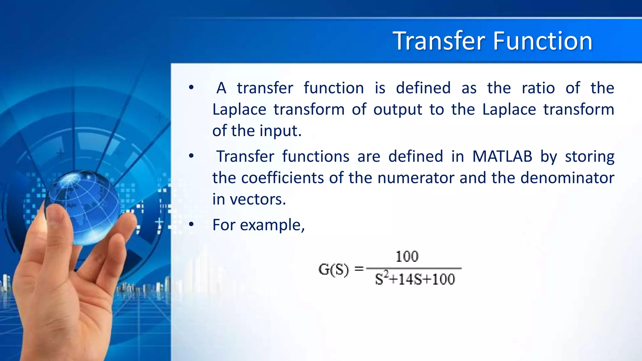
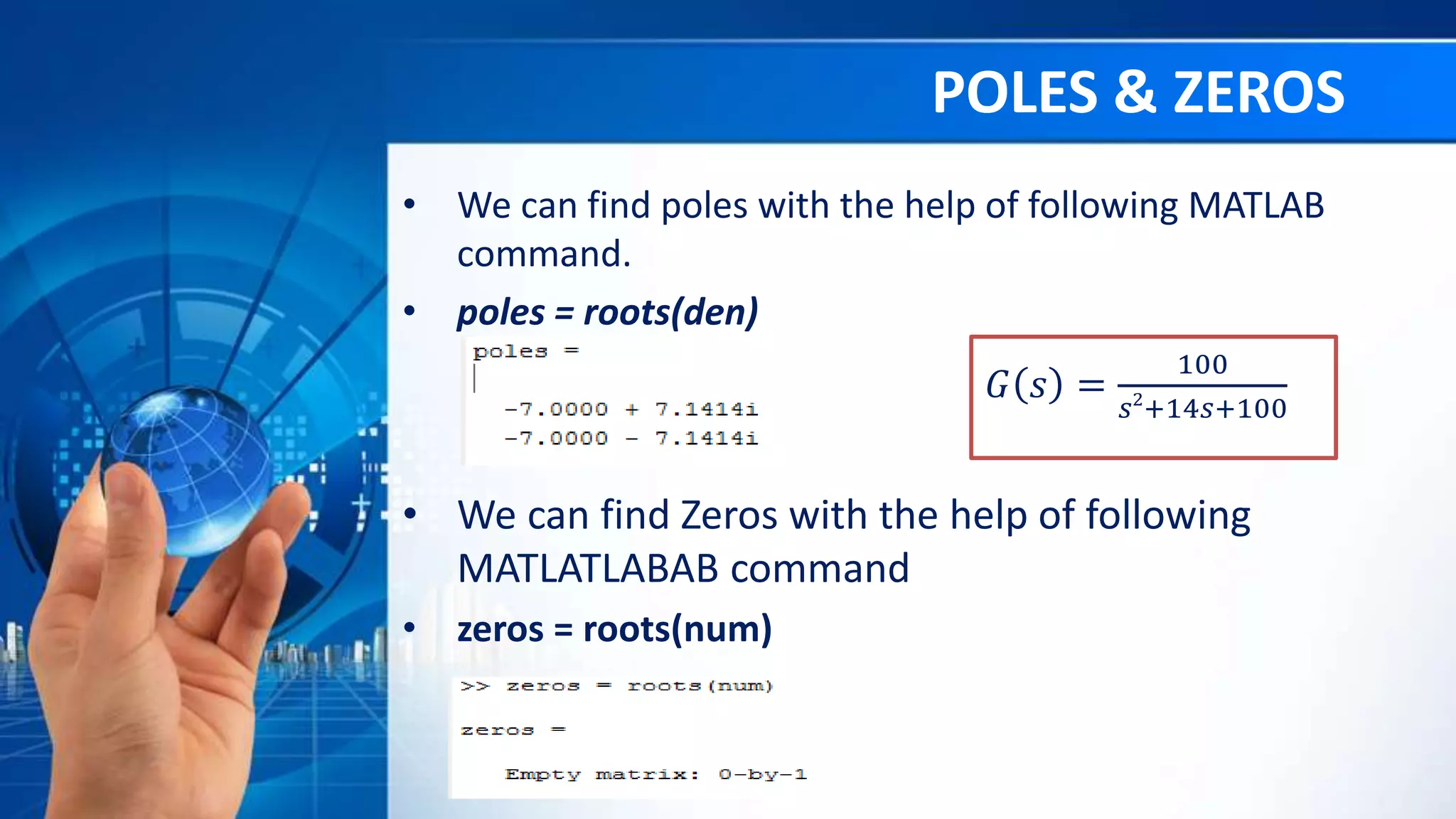
• 𝐺 𝑠 =
100
𝑠2
+14𝑠+100
• Here we type the following code
• num = 100;
• den = [1 14 100];
• To check your entry you can
use the command printsys
as shown below:
– printsys(num,den);
– Or G=tf(num,den)

12. POLES & ZEROS
• We can find poles with the help of following MATLAB
command.
• poles = roots(den)
𝐺 𝑠 =
100
𝑠2
+14𝑠+100
• We can find Zeros with the help of following
MATLATLABAB command
• zeros = roots(num)

13. PZMAP
• To plot the poles and zeros of any transfer function
there is a built in function pzmap in the MATLAB
• pzmap(num,den)

14. MULTIPLICATION OF TRANSFER FUNCTIONS
• num1 = [1 0];
• den1 = [9 17];
• num2 = 9*[1 3];
• den2 = [2 9 27];
• [num, den] = series (num1,den1,num2,den2);
printsys(num,den);

15. CLOSED-LOOP TRANSFER FUNCTION
• num = 9;
• den = [1 5];
• [numt,dent] = cloop(num,den,-1);
• printsys(numt,dent)

16. TIME RESPONSE OF CONTROL SYSTEM

17. TIME RESPONSE OF A CONTROL SYSTEM
• Step Response
• G(S)=
𝟏𝟎𝟎
𝑺 𝟐
+𝟏𝟒𝑺+𝟏𝟎𝟎
• To find the step response of the system
• num = 100;
• den = [1 14 100];
• step(num,den)

18. IMPULSE RESPONSE
• G(S)=
𝟏𝟎𝟎
S2+14S+100
• To find the step response of the system
• num = 100;
• den = [1 14 100];
• impulse(num,den)

19. Ramp Response
• G(S)=
100
S2+14S+100
• To find the ramp response of the system:
• t = 0:0.01:10;
• r = t;
• num = 100;
• den = [1 14 100];
• lsim(num,den,r,t)

21. TRANSFER FUNCTION TO STATE SPACE
• num = [12 59];
•
• den = [1 6 8];
•
• [A,B,C,D] = tf2ss(num,den);
•
• printsys(A,B,C,D)

22. STATE SPACE TO TRANSFER FUNCTION
• A = [-5 -1; 3 -1]
• B = [1 ; 0];
• C = [1 2];
• D = [0];
• [num,den]= ss2tf(A,B,C,D);
•
• printsys(num,den)

23. ANY QUESTION?