MATLAB is a high-level programming language and computing environment used for numerical computations, visualization, and programming. The document discusses MATLAB's capabilities including its toolboxes, plotting functions, control structures, M-files, and user-defined functions. MATLAB is useful for engineering and scientific calculations due to its matrix-based operations and built-in functions.

2. • The workshop covers basic MATLAB
commands that are used in introductory
Electrical Circuits and Machine analysis

3. • In this workshop you will learn a few of the
basic functions of MATLAB.
• First we will start working with basic numbers,
formats, demos, mathematical functions,
setting variables, matrices and generating
plots by using the plot functions.
• Brief overview of how to generate scripts in
MATLAB called M-files.

4. • MATLAB, which stands for MATRIX
LABORATORY, is a powerful, general-purpose
system or environment for doing
mathematics, scientific and engineeng
calculations.
• MATLAB is a "High-Performance Numeric
Computation and Visualization Software"
package.

5. • FORTRAN:
real*8 A(10,10), B(10,10), C(10,10)
do i=1,10
do j=1,10
C(i,j) = A(i,j) + B(i,j)
10 continue
20 continue
• MATLAB:
C = A + B

6. • MATLAB is an interactive system whose basic
data is a matrix that does not require
dimensioning.

7. What is Matlab?
• Matlab is basically a high level language which has
many specialized toolboxes for making things
easier for us
• How high?
Assembly
High Level
Languages such as
C, Pascal etc.
Matlab

8. Introduction to Matlab

9. Outline:
What is Matlab?
• Matlab Screen
• Variables, array, matrix, indexing
• Operators (Arithmetic, relational, logical )
• Display Facilities
• Flow Control
• Using of M-File
• Writing User Defined Functions
• Conclusion

10. What is Matlab?
• Matlab is basically a high level language which
has many specialized toolboxes for making
things easier for us
• How high?
Assembly
High Level
Languages such as
C, Pascal etc.
Matlab

11. What are we interested in?
• Matlab is too broad for our purposes in this
course.
• The features we are going to require is
Matlab
Command
Line
m-files
functions
mat-files
Command execution
like DOS command
window
Series of
Matlab
commands
Input
Output
capability
Data
storage/
loading

12. Matlab Screen
• Command Window
– type commands
• Current Directory
– View folders and m-files
• Workspace
– View program variables
– Double click on a variable
to see it in the Array Editor
• Command History
– view past commands
– save a whole session
using diary

13. Variables
• No need for types. i.e.,
• All variables are created with double precision unless
specified and they are matrices.
• After these statements, the variables are 1x1 matrices with
double precision
int a;
double b;
float c;
Example:
>>x=5;
>>x1=2;

14. Array, Matrix
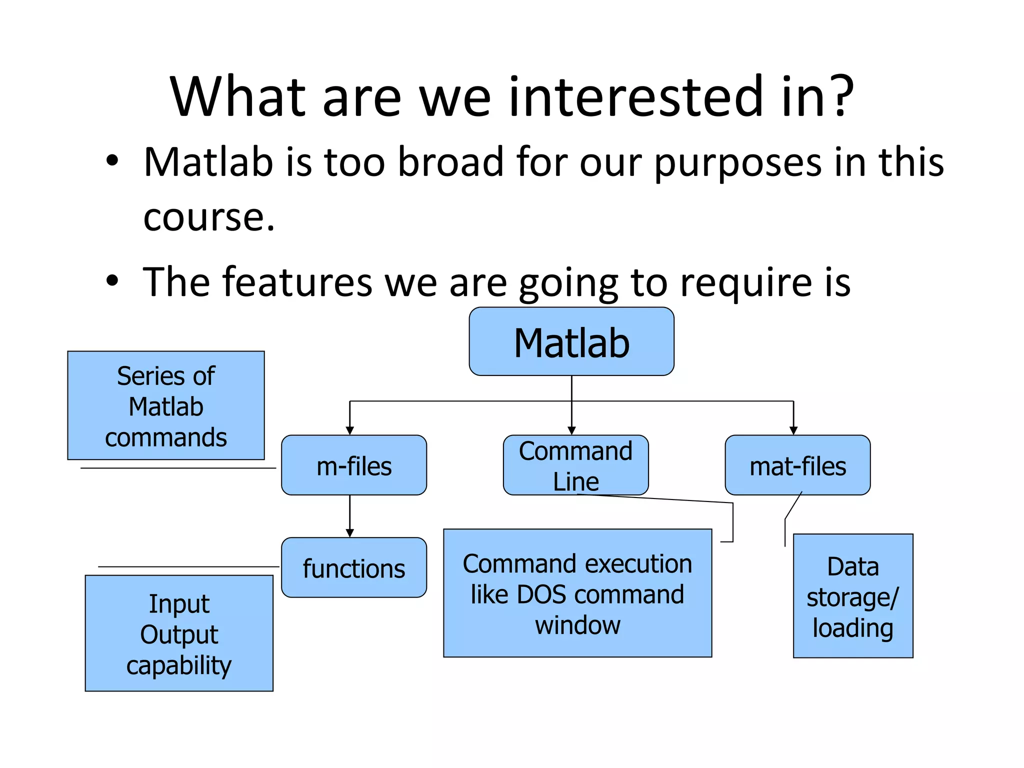
• a vector x = [1 2 5 1]
x =
1 2 5 1
• a matrix x = [1 2 3; 5 1 4; 3 2 -1]
x =
1 2 3
5 1 4
3 2 -1
• transpose y = x’ y =
1
2
5
1

15. Long Array, Matrix
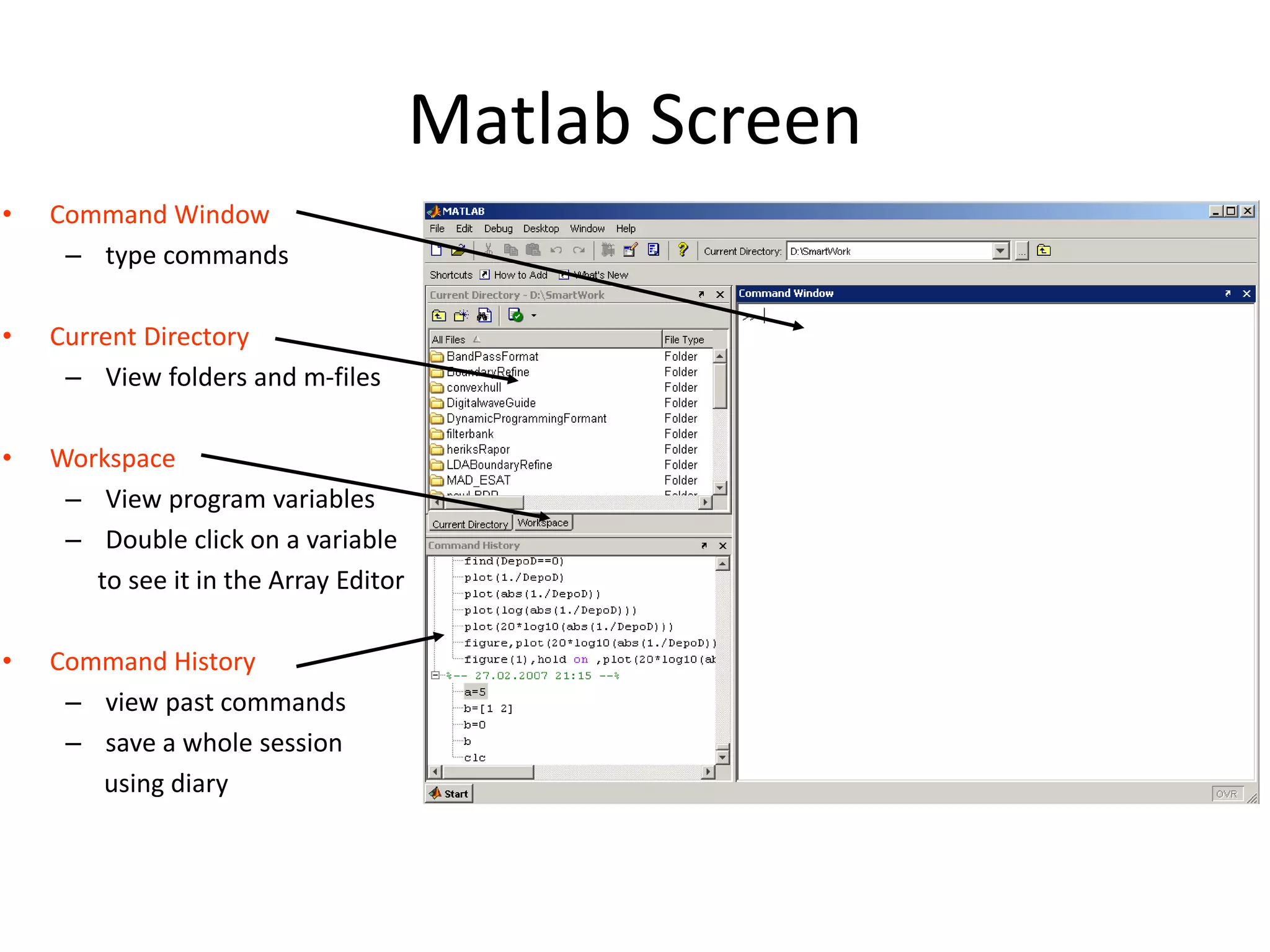
• t =1:10
t =
1 2 3 4 5 6 7 8 9 10
• k =2:-0.5:-1
k =
2 1.5 1 0.5 0 -0.5 -1
• B = [1:4; 5:8]
x =
1 2 3 4
5 6 7 8

16. Generating Vectors from functions
• zeros(M,N) MxN matrix of zeros
• ones(M,N) MxN matrix of ones
• rand(M,N) MxN matrix of uniformly
distributed random
numbers on (0,1)
x = zeros(1,3)
x =
0 0 0
x = ones(1,3)
x =
1 1 1
x = rand(1,3)
x =
0.9501 0.2311 0.6068

17. Matrix Index
• The matrix indices begin from 1 (not 0 (as in C))
• The matrix indices must be positive integer
Given:
A(-2), A(0)
Error: ??? Subscript indices must either be real positive integers or logicals.
A(4,2)
Error: ??? Index exceeds matrix dimensions.

18. Concatenation of Matrices
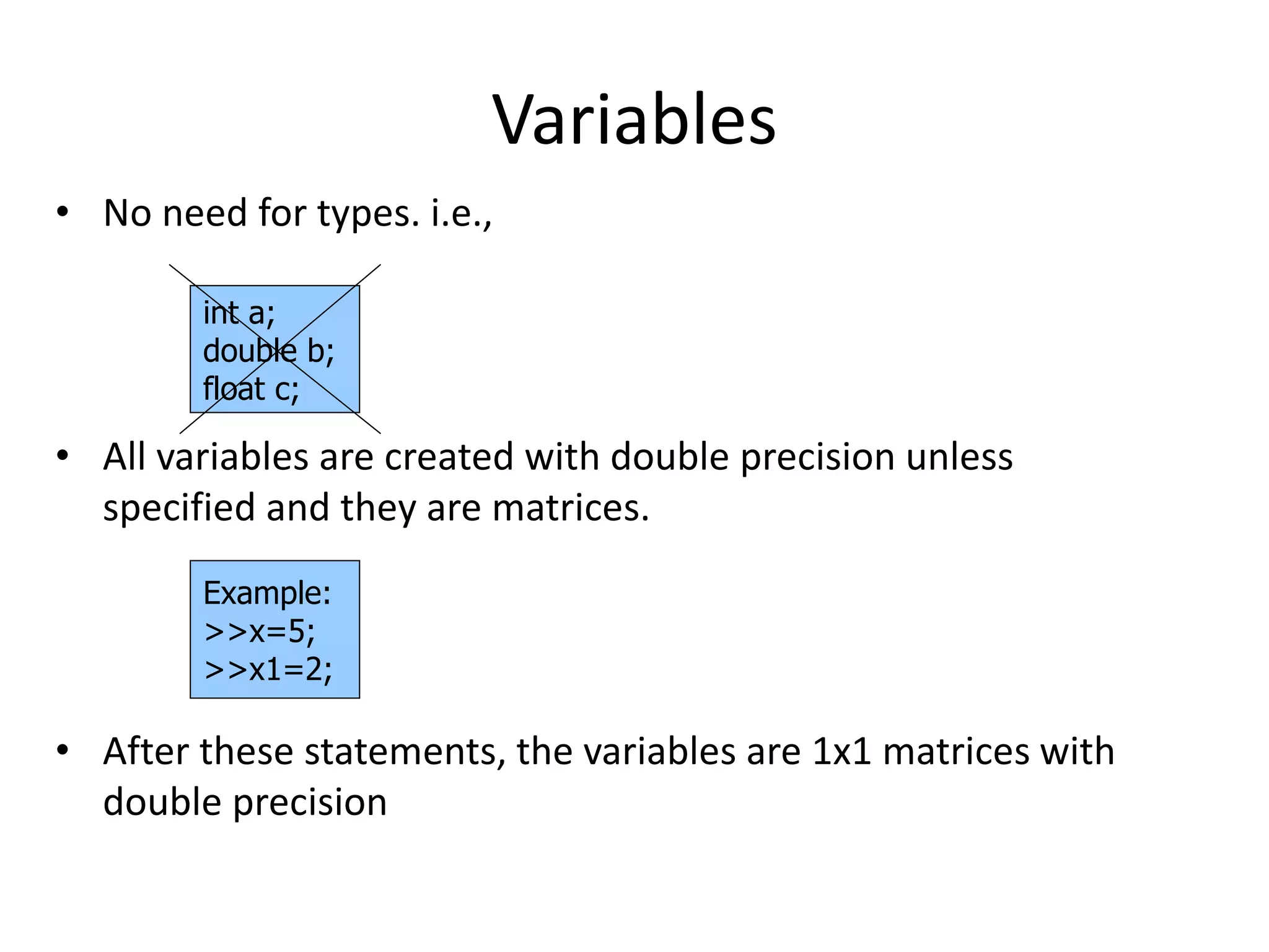
• x = [1 2], y = [4 5], z=[ 0 0]
A = [ x y]
1 2 4 5
B = [x ; y]
1 2
4 5
C = [x y ;z]
Error:
??? Error using ==> vertcat CAT arguments dimensions are not consistent.

19. Operators (arithmetic)
+ addition
- subtraction
* multiplication
/ division
^ power
‘ complex conjugate transpose

20. Matrices Operations
Given A and B:
Addition Subtraction Product Transpose

21. Operators (Element by Element)
.*element-by-element multiplication
./ element-by-element division
.^element-by-element power

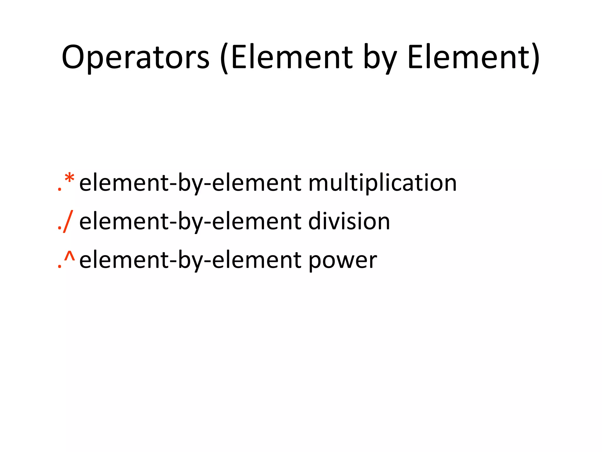
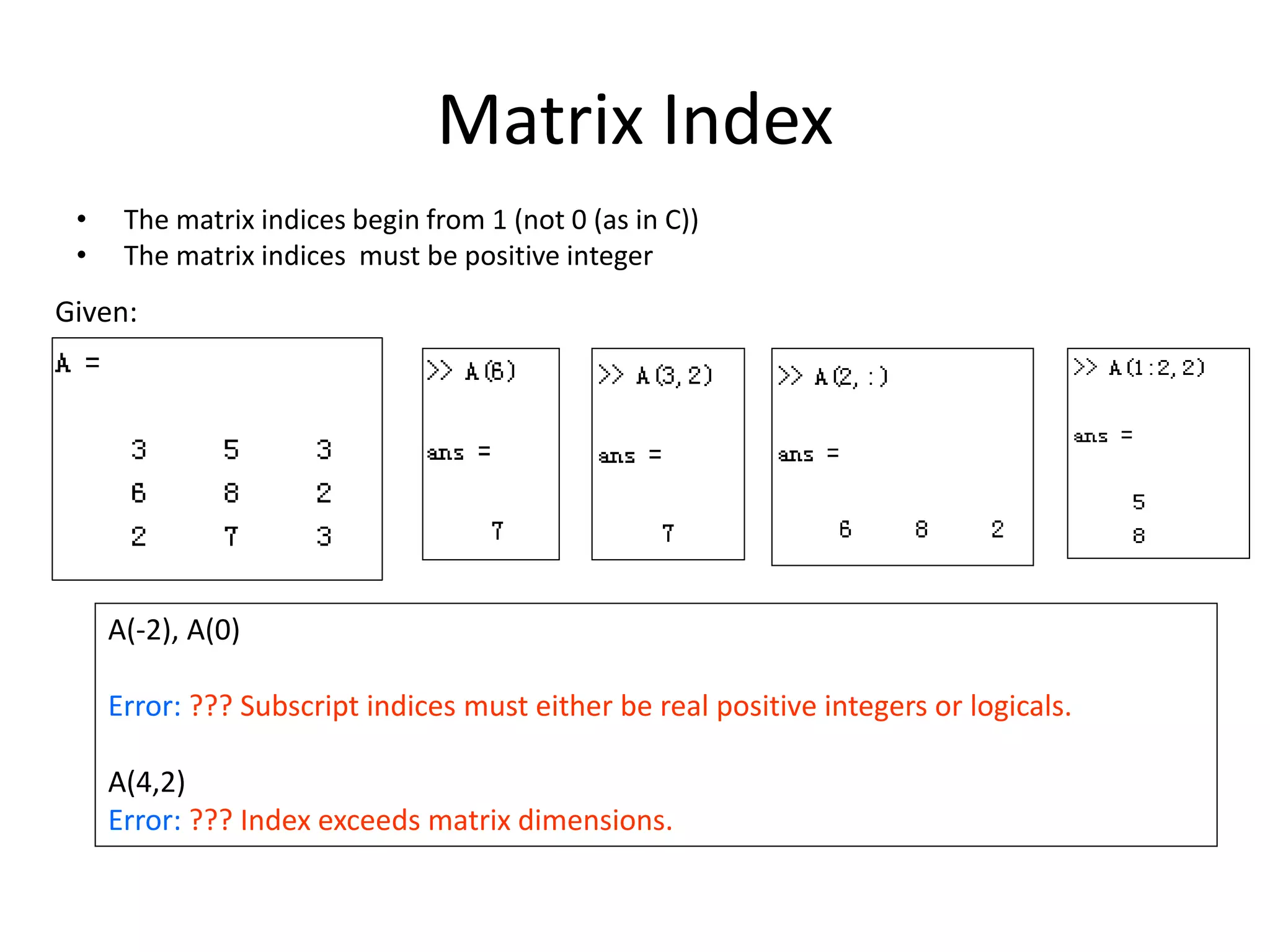
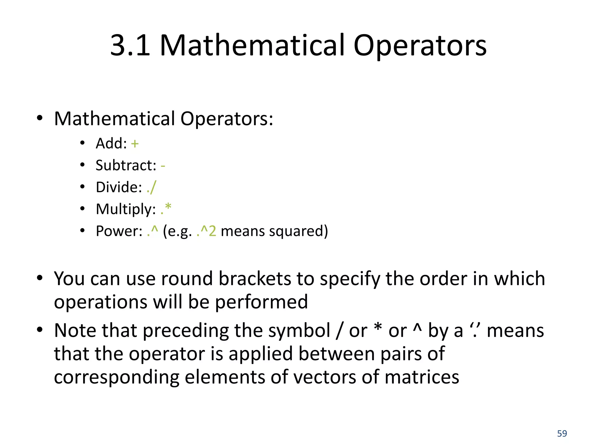
22. The use of “.” – “Element” Operation
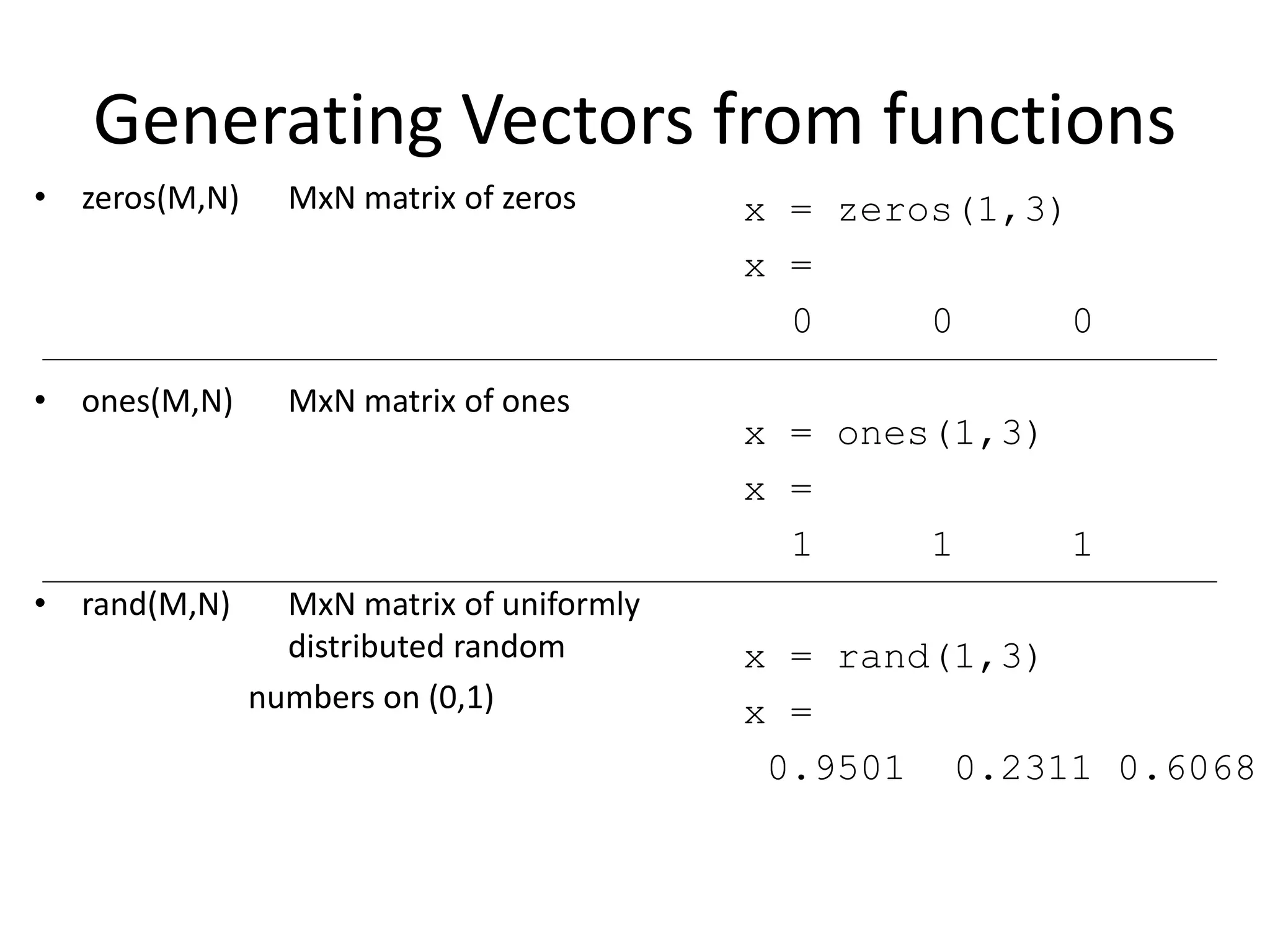
K= x^2
Erorr:
??? Error using ==> mpower Matrix must be square.
B=x*y
Erorr:
??? Error using ==> mtimes Inner matrix dimensions must agree.
A = [1 2 3; 5 1 4; 3 2 1]
A =
1 2 3
5 1 4
3 2 -1
y = A(3 ,:)
y=
3 4 -1
b = x .* y
b=
3 8 -3
c = x . / y
c=
0.33 0.5 -3
d = x .^2
d=
1 4 9
x = A(1,:)
x=
1 2 3

23. Basic Task: Plot the function sin(x) between
0≤x≤4π
• Create an x-array of 100 samples between 0 and
4π.
• Calculate sin(.) of the x-array
• Plot the y-array
>>x=linspace(0,4*pi,100);
>>y=sin(x);
>>plot(y)
0 10 20 30 40 50 60 70 80 90 100
-1
-0.8
-0.6
-0.4
-0.2
0
0.2
0.4
0.6
0.8
1

24. Plot the function e-x/3sin(x) between 0≤x≤4π
• Create an x-array of 100 samples between 0
and 4π.
• Calculate sin(.) of the x-array
• Calculate e-x/3 of the x-array
• Multiply the arrays y and y1
>>x=linspace(0,4*pi,100);
>>y=sin(x);
>>y1=exp(-x/3);
>>y2=y*y1;

25. Plot the function e-x/3sin(x) between 0≤x≤4π
• Multiply the arrays y and y1 correctly
• Plot the y2-array
>>y2=y.*y1;
>>plot(y2)
0 10 20 30 40 50 60 70 80 90 100
-0.3
-0.2
-0.1
0
0.1
0.2
0.3
0.4
0.5
0.6
0.7

26. Display Facilities
• plot(.)
• stem(.)
Example:
>>x=linspace(0,4*pi,100);
>>y=sin(x);
>>plot(y)
>>plot(x,y)
Example:
>>stem(y)
>>stem(x,y)
0 10 20 30 40 50 60 70 80 90 100
-0.3
-0.2
-0.1
0
0.1
0.2
0.3
0.4
0.5
0.6
0.7
0 10 20 30 40 50 60 70 80 90 100
-0.3
-0.2
-0.1
0
0.1
0.2
0.3
0.4
0.5
0.6
0.7

27. Display Facilities
• title(.)
• xlabel(.)
• ylabel(.)
>>title(‘This is the sinus function’)
>>xlabel(‘x (secs)’)
>>ylabel(‘sin(x)’)
0 10 20 30 40 50 60 70 80 90 100
-1
-0.8
-0.6
-0.4
-0.2
0
0.2
0.4
0.6
0.8
1
This is the sinus function
x (secs)
sin(x)

28. Operators (relational, logical)
• == Equal to
• ~= Not equal to
• < Strictly smaller
• > Strictly greater
• <= Smaller than or equal to
• >= Greater than equal to
• & And operator
• | Or operator

29. Flow Control
• if
• for
• while
• break
• ….

30. Control Structures
• If Statement Syntax
if (Condition_1)
Matlab Commands
elseif (Condition_2)
Matlab Commands
elseif (Condition_3)
Matlab Commands
else
Matlab Commands
end
Some Dummy Examples
if ((a>3) & (b==5))
Some Matlab Commands;
end
if (a<3)
Some Matlab Commands;
elseif (b~=5)
Some Matlab Commands;
end
if (a<3)
Some Matlab Commands;
else
Some Matlab Commands;
end

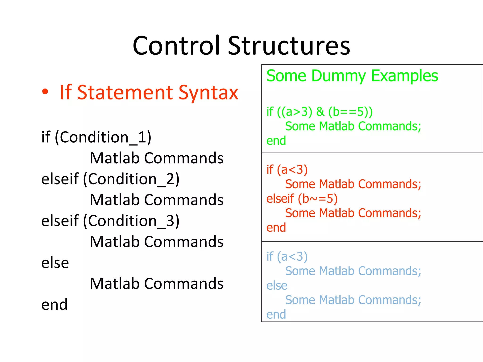
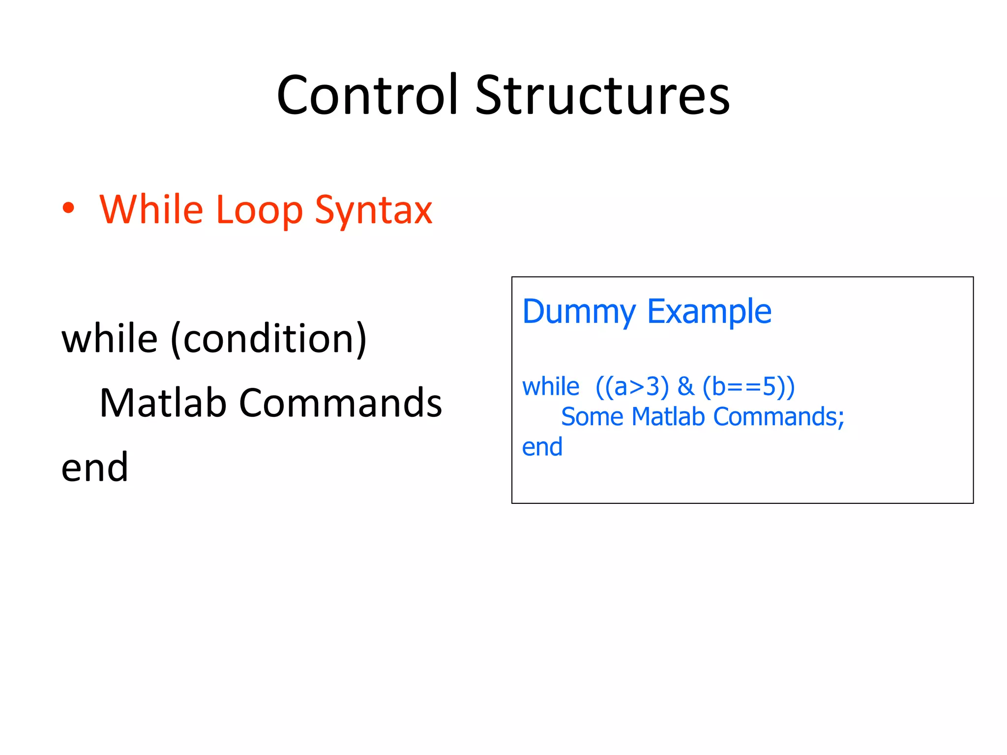
31. Control Structures
• For loop syntax
for i=Index_Array
Matlab Commands
end
Some Dummy Examples
for i=1:100
Some Matlab Commands;
end
for j=1:3:200
Some Matlab Commands;
end
for m=13:-0.2:-21
Some Matlab Commands;
end
for k=[0.1 0.3 -13 12 7 -9.3]
Some Matlab Commands;
end

32. Control Structures
• While Loop Syntax
while (condition)
Matlab Commands
end
Dummy Example
while ((a>3) & (b==5))
Some Matlab Commands;
end

33. Use of M-File
Click to create a
new M-File
• Extension “.m”
• A text file containing script or function or program to run

34. Use of M-File
If you include “;” at the
end of each statement,
result will not be shown
immediately
Save file as Denem430.m

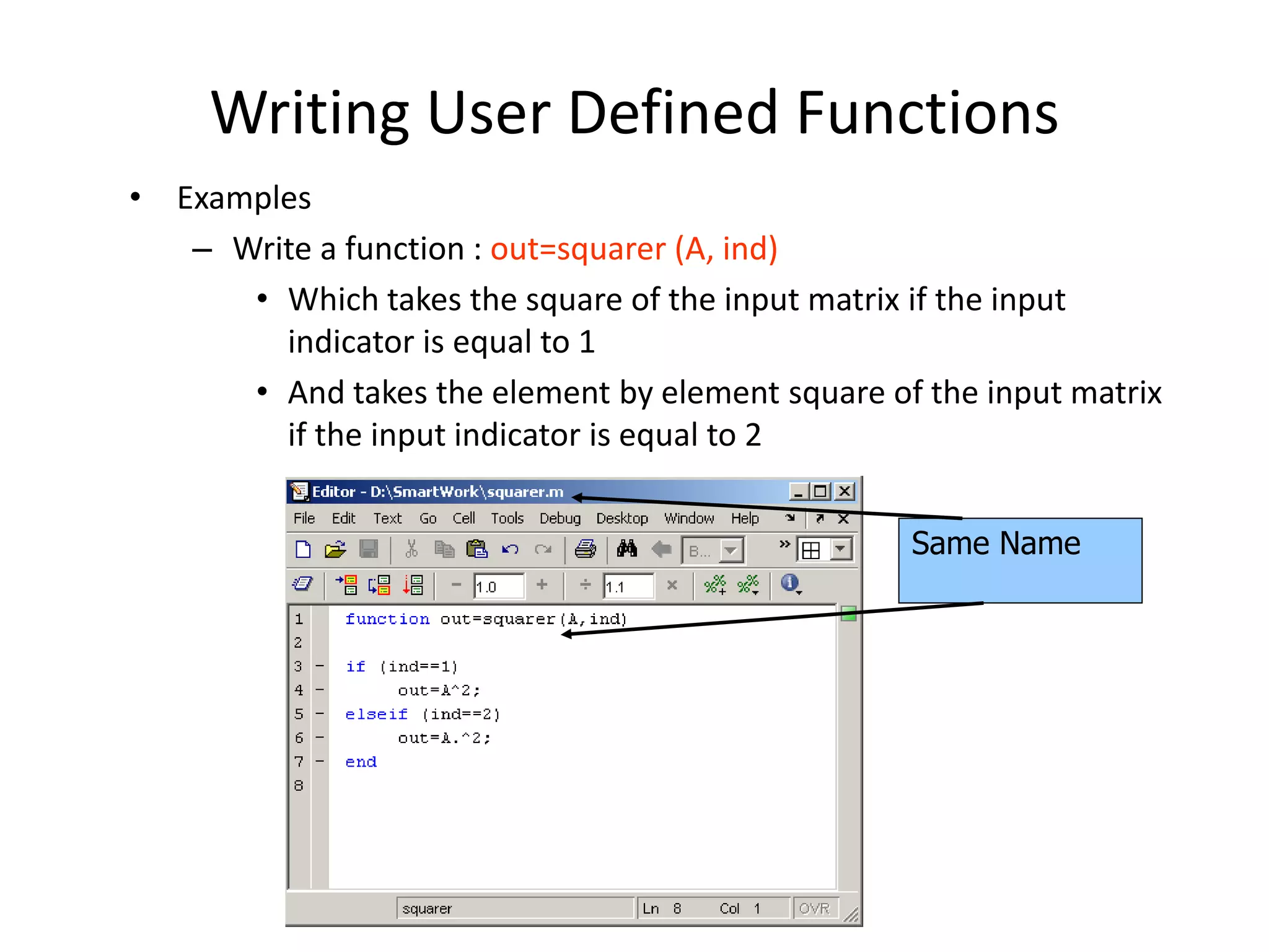
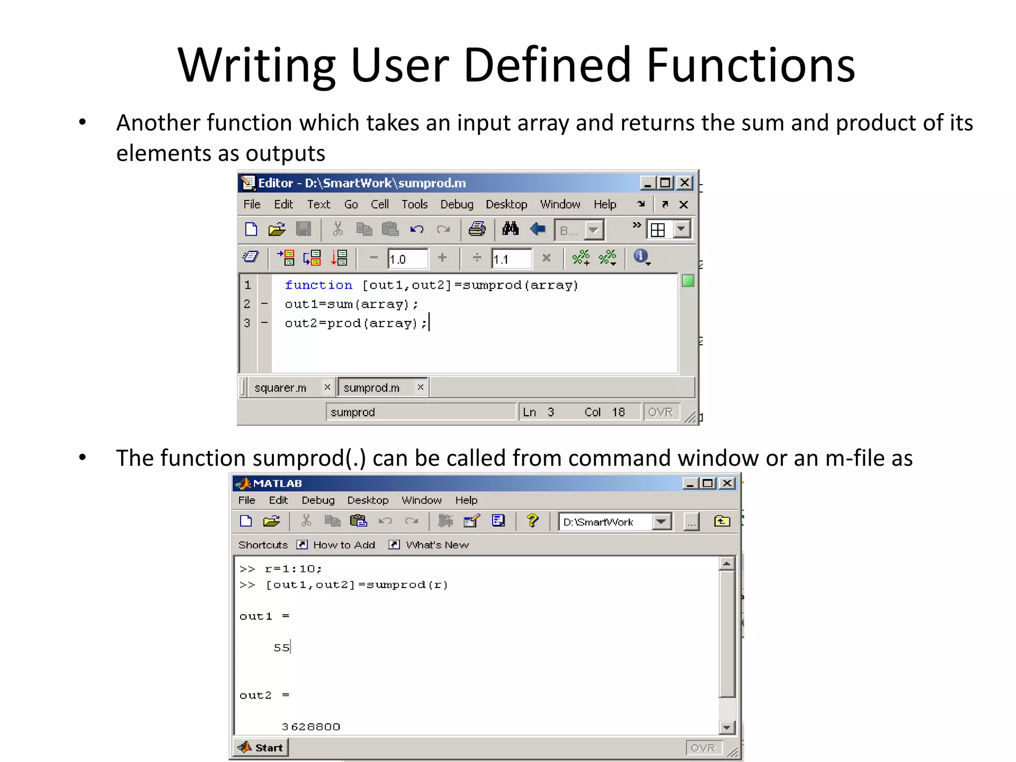
35. Writing User Defined Functions
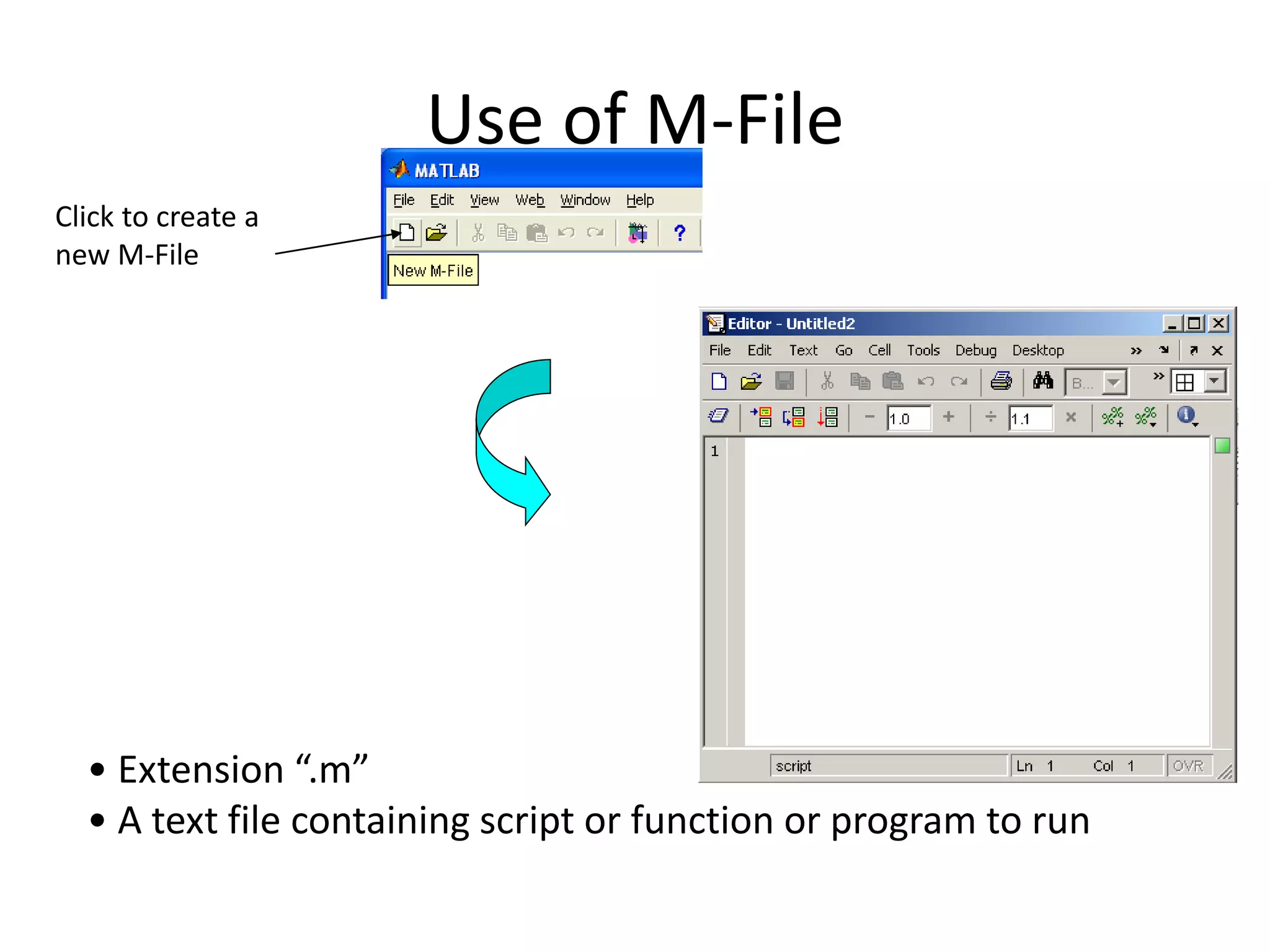
• Functions are m-files which can be executed by specifying
some inputs and supply some desired outputs.
• The code telling the Matlab that an m-file is actually a function
is
• You should write this command at the beginning of the m-file
and you should save the m-file with a file name same as the
function name
function out1=functionname(in1)
function out1=functionname(in1,in2,in3)
function [out1,out2]=functionname(in1,in2)

36. Writing User Defined Functions
• Examples
– Write a function : out=squarer (A, ind)
• Which takes the square of the input matrix if the input
indicator is equal to 1
• And takes the element by element square of the input matrix
if the input indicator is equal to 2
Same Name

37. Writing User Defined Functions
• Another function which takes an input array and returns the sum and product of its
elements as outputs
• The function sumprod(.) can be called from command window or an m-file as

38. Notes:
• “%” is the neglect sign for Matlab (equaivalent
of “//” in C). Anything after it on the same line
is neglected by Matlab compiler.
• Sometimes slowing down the execution is
done deliberately for observation purposes.
You can use the command “pause” for this
purpose
pause %wait until any key
pause(3) %wait 3 seconds

39. Useful Commands
• The two commands used most by Matlab
users are
>>help functionname
>>lookfor keyword

40. Questions
• ?
• ?
• ?
• ?
• ?

41. Thank You…

42. • MATLAB has a number of add-on software modules,
called toolbox , that perform more specialized
computations.
• Electrical Engineering
Signal Processing- Image Processing Communications -
System Identification - Wavelet Filter Design
• Control Design
• Control System - Fuzzy Logic - Robust Control - µ-
Analysis and Synthesis - LMI Control - Model Predictive
Control Model-Based Calibration
• More than 60 toolboxes!

44. • In Windows systems MATLAB is started by
double-clicking the mouse on the appropriate
icon.

45. MATLAB has many toolboxes:
• Control toolbox is one of the important
toolbox in MATLAB.
• RLC Circuit Response,
• Gain and Phase Margins,
• Notch Filter Discrete,
• PID and ...

46. • Simulink has the ability to simulate a large
range of systems, from very simple to
extraordinarily complex. The Model and
demonstrations that you will see in this
section include both simple and complex
systems.
• Imitate the appearance or character

47. • Simulink has the ability to simulate a large
range of systems, in the menu of Simulation
we have:
• Pause.
• Stop,
• Simulation Parameters,
• Start,

48. • MATLAB is a numeric computation software for
engineering and scientific calculations.
• MATLAB is increasingly being used by students,
researchers, practicing engineers and technicians.
The causes of MATLAB popularity are legion.
Among them are its iterative mode of operation,
built-in functions, simple programming, rich set
of graphing facilities, possibilities for writing
additional functions, and its extensive toolboxes.

49. • MATLAB is a high-level language whose basic
data type is a matrix that does not require
dimensioning. There is no compilation and
linking as is done in high-level languages, such
as C or FORTRAN. Computer solutions in
MATLAB seem to be much quicker than those
of a high-level language such as C or
FORTRAN. All computations are performed in
complex-valued double precision arithmetic to
guarantee high accuracy.

50. • MATLAB is a numeric computation software for
engineering and scientific calculations.
• The name MATLAB stands for MATRIX
LABORATORY.
• MATLAB is primarily a tool for matrix
computations. It was developed by John Little and
Cleve Moler of MathWorks, Inc. MATLAB was
originally written to provide easy access to the
matrix computation software packages LINPACK
and EISPACK.

57. • The Language
• The MATLAB language is a high-level matrix/array language with
control flow statements, functions, data structures, input/output,
and object-oriented programming features.
• Graphics
• MATLAB has extensive facilities for displaying vectors and matrices
as graphs, as well as editing and printing these graphs. It also
includes functions that allow you to customize the appearance of
graphics as well as build complete graphical user interfaces on your
MATLAB applications.
• External Interfaces
• The external interfaces library allows you to write C and Fortran
programs that interact with MATLAB.

58. • Plotting Multiple Data Sets in One Graph
– Multiple x-y pair arguments create multiple graphs with a
single call to plot.
For example: x = 0:pi/100:2*pi;
y = sin(x);
y2 = sin(x-.25);
y3 = sin(x-.5);
plot(x,y,x,y2,x,y3)

59. 3.1 Mathematical Operators
• Mathematical Operators:
• Add: +
• Subtract: -
• Divide: ./
• Multiply: .*
• Power: .^ (e.g. .^2 means squared)
• You can use round brackets to specify the order in which
operations will be performed
• Note that preceding the symbol / or * or ^ by a ‘.’ means
that the operator is applied between pairs of
corresponding elements of vectors of matrices
59

60. 3.1 Operation on matrices
• Multiplication of matrices with * calculates inner
products between rows and columns
• To transpose a matrix, use ‘
• det(A) calculates the determinant of a matrix A
• inv(A) calculates the inverse of a matrix A
• pinv(A) calculates the pseudo-inverse of A
• …and so on

61. 3.2 Logical Operators
– You can use Logical Indexing to find data that
conforms to some limitations
– Logical Operators:
• Greater Than: >
• Less Than: <
• Greater Than or Equal To: >=
• Less Than or Equal To: <=
• Is Equal: ==
• Not Equal To: ~=
61

62. 4 Functions
• MATLAB has many built in functions which make it easy to perform a
variety of statistical operations
– sum – Sums the content of the variable passed
– prod – Multiplies the content of the variable passed
– mean – Calculates the mean of the variable passed
– median – Calculates the median of the variable passed
– mode – Calculates the Mode of the variable passed
– std – Calculates the standard deviation of the variable passed
– sqrt – Calculates the square root of the variable passed
– max – Finds the maximum of the data
– min – Finds the minimum of the data
– size – Gives the size of the variable passed
62

63. 4 Special functions
• There are a number of special functions that provide
useful constants
– pi = 3.14159265….
– i or j = square root of -1
– Inf = infinity
– NaN = not a number

64. 5 Plotting
• The plot function can be used in different ways:
>> plot(data)
>> plot(x, y)
>> plot(data, ‘r.-’)
• In the last example the line style is defined
Colour: r, b, g, c, k, y etc.
Point style: . + * x o > etc.
Line style: - -- : .-
– Type ‘help plot’ for a full list of the options
64