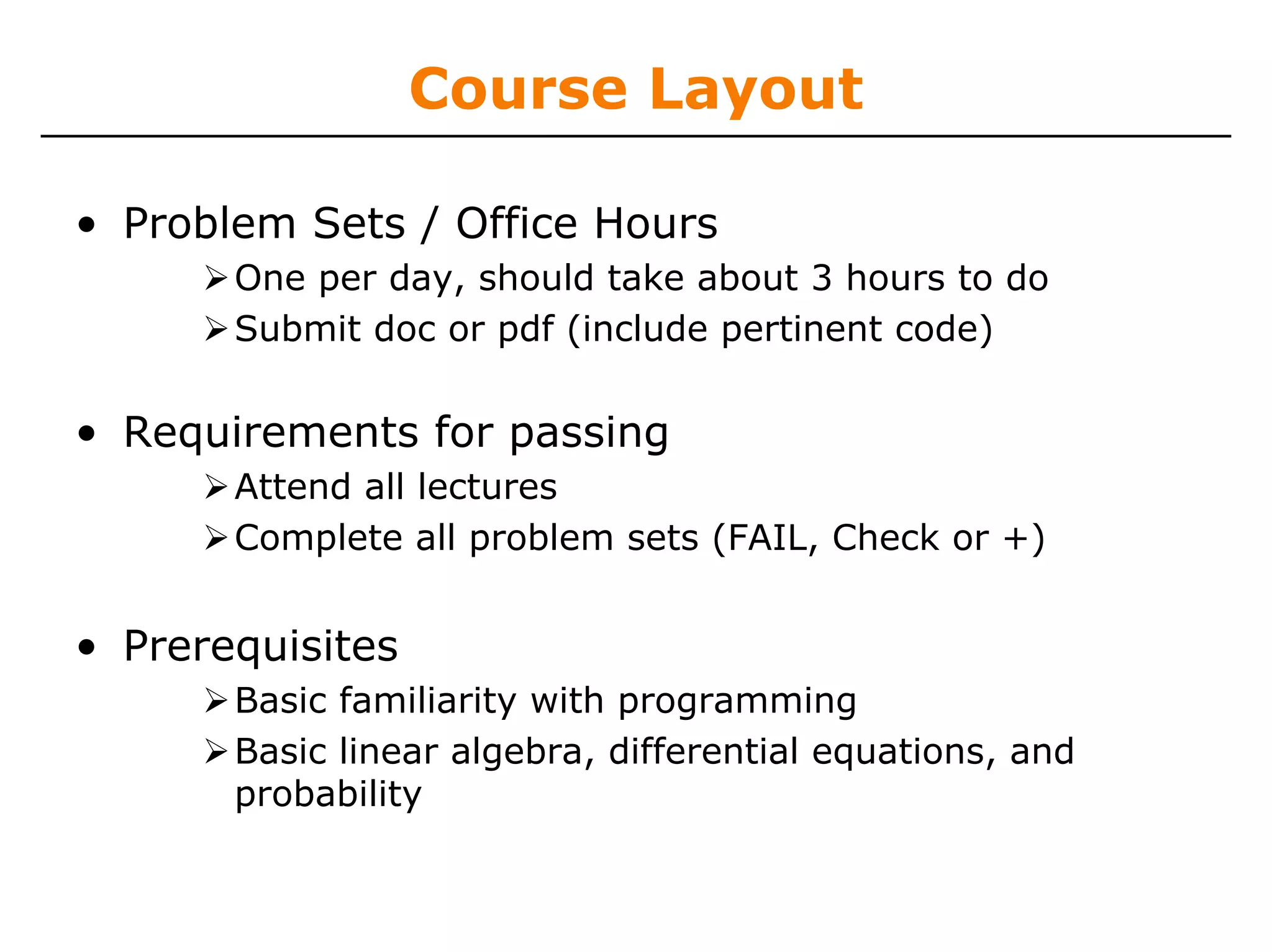
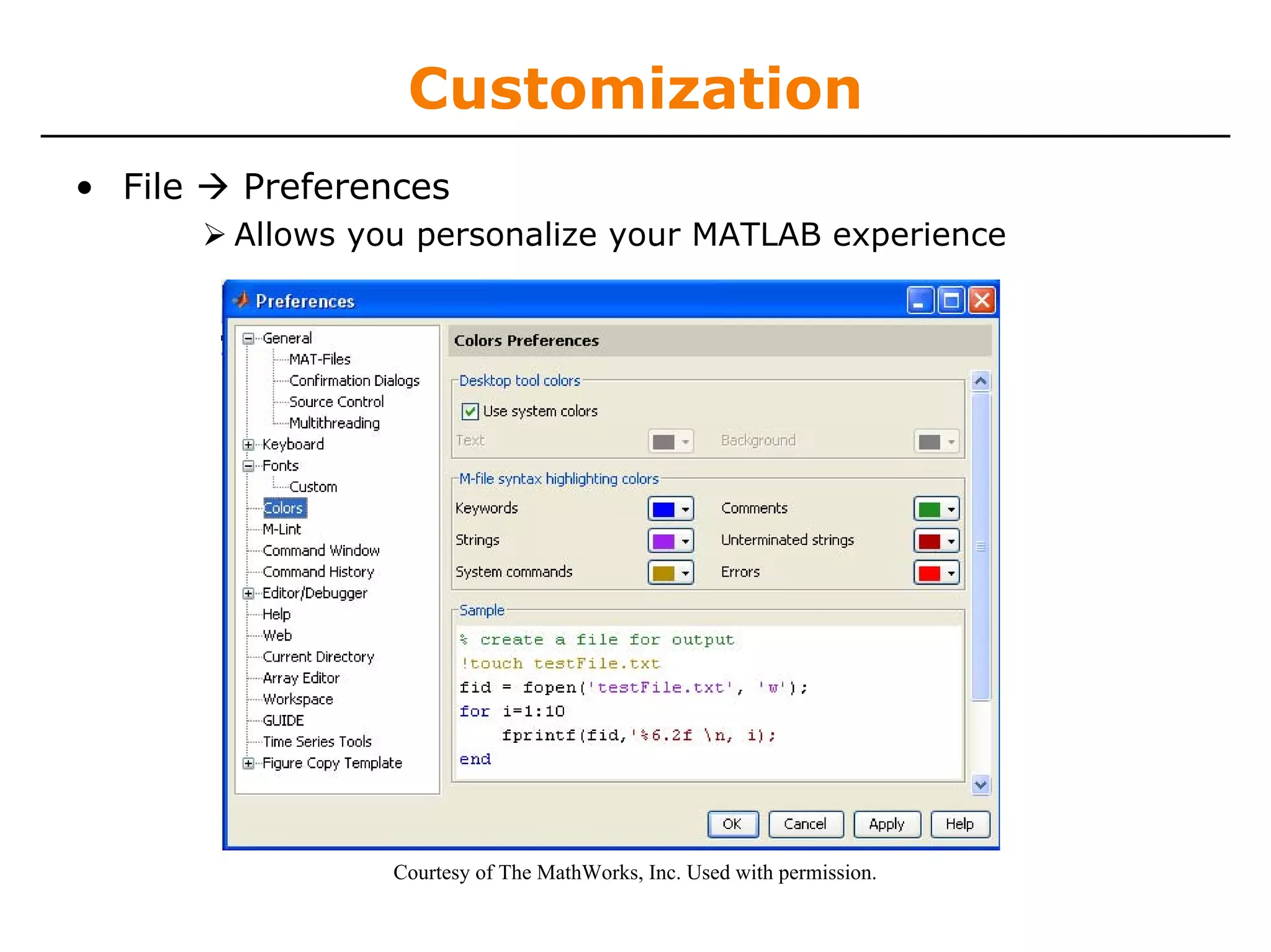
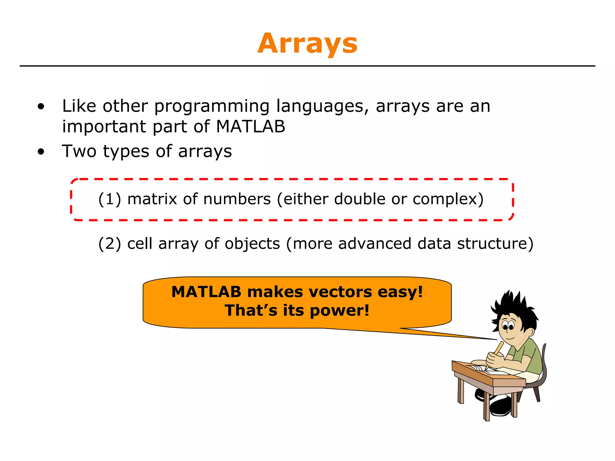
![Row Vectors
• Row vector: comma or space separated values between
brackets
» row = [1 2 5.4 -6.6];
» row = [1, 2, 5.4, -6.6];
• Command window:
• Workspace:
Courtesy of The MathWorks, Inc. Used with permission.](https://image.slidesharecdn.com/matlablec1-100301012417-phpapp02/75/Matlab-lec1-17-2048.jpg)
![Column Vectors
• Column vector: semicolon separated values between
brackets
» column = [4;2;7;4];
• Command window:
• Workspace:
Courtesy of The MathWorks, Inc. Used with permission.](https://image.slidesharecdn.com/matlablec1-100301012417-phpapp02/75/Matlab-lec1-18-2048.jpg)
![Matrices
• Make matrices like vectors
⎡1 2⎤
• Element by element a=⎢
» a= [1 2;3 4]; ⎣3 4⎥
⎦
• By concatenating vectors or matrices (dimension matters)
» a = [1 2];
» b = [3 4];
» c = [5;6];
» d = [a;b];
» e = [d c];
» f = [[e e];[a b a]];](https://image.slidesharecdn.com/matlablec1-100301012417-phpapp02/75/Matlab-lec1-19-2048.jpg)
![Exercise: Variables
• Do the following 5 things:
Create the variable r as a row vector with values 1 4
7 10 13
Create the variable c as a column vector with values
13 10 7 4 1
Save these two variables to file varEx
clear the workspace
load the two variables you just created
» r=[1 4 7 10 13];
» c=[13; 10; 7; 4; 1];
» save varEx r c
» clear r c
» load varEx](https://image.slidesharecdn.com/matlablec1-100301012417-phpapp02/75/Matlab-lec1-21-2048.jpg)
![transpose
• The transpose operators turns a column vector into a row
vector and vice versa
» a = [1 2 3 4]
» transpose(a)
• Can use dot-apostrophe as short-cut
» a.'
• The apostrophe gives the Hermitian-transpose, i.e.
transposes and conjugates all complex numbers
» a = [1+j 2+3*j]
» a'
» a.'
• For vectors of real numbers .' and ' give same result](https://image.slidesharecdn.com/matlablec1-100301012417-phpapp02/75/Matlab-lec1-28-2048.jpg)
![Addition and Subtraction
• Addition and subtraction are element-wise; sizes must
match (unless one is a scalar):
[12 3 32 −11] ⎡ 12 ⎤ ⎡ 3 ⎤ ⎡ 9 ⎤
⎢ 1 ⎥ ⎢ −1⎥ ⎢ 2 ⎥
+ [ 2 11 −30 32] ⎢ ⎥−⎢ ⎥ = ⎢ ⎥
⎢ −10 ⎥ ⎢13 ⎥ ⎢ −23⎥
= [14 14 2 21] ⎢ ⎥ ⎢ ⎥ ⎢ ⎥
⎣ 0 ⎦ ⎣33⎦ ⎣ −33⎦
• The following would give an error
» c = row + column
• Use the transpose to make sizes compatible
» c = row’ + column
» c = row + column’
• Can sum up or multiply elements of vector
» s=sum(row);
» p=prod(row);](https://image.slidesharecdn.com/matlablec1-100301012417-phpapp02/75/Matlab-lec1-29-2048.jpg)
![Element-Wise Functions
• All the functions that work on scalars also work on vectors
» t = [1 2 3];
» f = exp(t);
is the same as
» f = [exp(1) exp(2) exp(3)];
• If in doubt, check a function’s help file to see if it handles
vectors elementwise
• Operators (* / ^) have two modes of operation
element-wise
standard](https://image.slidesharecdn.com/matlablec1-100301012417-phpapp02/75/Matlab-lec1-30-2048.jpg)
![Operators: element-wise
• To do element-wise operations, use the dot. BOTH
dimensions must match (unless one is scalar)!
» a=[1 2 3];b=[4;2;1];
» a.*b, a./b, a.^b all errors
» a.*b’, a./b’, a.^(b’) all valid
⎡ 4⎤ ⎡1 1 1 ⎤ ⎡1 2 3⎤ ⎡ 1 2 3⎤
⎢ 2 2 2 ⎥ .* ⎢1 2 3⎥ = ⎢ 2 4 6 ⎥
[1 2 3] .* ⎢ 2⎥ = ERROR
⎢ ⎥ ⎢ ⎥ ⎢ ⎥ ⎢ ⎥
⎢1 ⎥
⎣ ⎦ ⎢ 3 3 3 ⎥ ⎢1 2 3⎥ ⎢ 3 6 9 ⎥
⎣ ⎦ ⎣ ⎦ ⎣ ⎦
⎡1 ⎤ ⎡ 4⎤ ⎡ 4⎤ 3 × 3.* 3 × 3 = 3 × 3
⎢ 2 ⎥ .* ⎢ 2 ⎥ = ⎢ 4 ⎥
⎢ ⎥ ⎢ ⎥ ⎢ ⎥
⎢ 3⎥ ⎢1 ⎥ ⎢ 3⎥
⎣ ⎦ ⎣ ⎦ ⎣ ⎦
⎡1 2 ⎤ ⎡12 22 ⎤
3 ×1.* 3 ×1 = 3 × 1 ⎢3 4 ⎥ .^ 2 = ⎢ 2 ⎥
⎣ ⎦ ⎣ 3 42 ⎦
Can be any dimension](https://image.slidesharecdn.com/matlablec1-100301012417-phpapp02/75/Matlab-lec1-31-2048.jpg)
![Operators: standard
• Multiplication can be done in a standard way or element-wise
• Standard multiplication (*) is either a dot-product or an outer-
product
Remember from linear algebra: inner dimensions must MATCH!!
• Standard exponentiation (^) implicitly uses *
Can only be done on square matrices or scalars
• Left and right division (/ ) is same as multiplying by inverse
Our recommendation: just multiply by inverse (more on this
later)
⎡ 4⎤ ⎡1 2 ⎤ ⎡1 2 ⎤ ⎡1 2 ⎤ ⎡1 1 1⎤ ⎡1 2 3⎤ ⎡3 6 9 ⎤
[1 2 3]* ⎢ 2⎥ = 11
⎢ ⎥
⎢3 4 ⎥
⎣ ⎦
^2=⎢ ⎥ * ⎢3 4 ⎥
⎣3 4 ⎦ ⎣ ⎦
⎢2 2 2⎥ * ⎢1 2 3⎥ = ⎢6 12 18 ⎥
⎢ ⎥ ⎢ ⎥ ⎢ ⎥
⎢1 ⎥
⎣ ⎦ Must be square to do powers ⎢3 3 3⎥ ⎢1 2 3⎥ ⎢9 18 27⎥
⎣ ⎦ ⎣ ⎦ ⎣ ⎦
1× 3* 3 ×1 = 1× 1 3 × 3* 3 × 3 = 3 × 3](https://image.slidesharecdn.com/matlablec1-100301012417-phpapp02/75/Matlab-lec1-32-2048.jpg)
![Exercise: Vector Operations
• Find the inner product between [1 2 3] and [3 5 4]
» a=[1 2 3]*[3 5 4]’
• Multiply the same two vectors element-wise
» b=[1 2 3].*[3 5 4]
• Calculate the natural log of each element of the resulting
vector
» c=log(b)](https://image.slidesharecdn.com/matlablec1-100301012417-phpapp02/75/Matlab-lec1-33-2048.jpg)
![Automatic Initialization
• Initialize a vector of ones, zeros, or random numbers
» o=ones(1,10)
row vector with 10 elements, all 1
» z=zeros(23,1)
column vector with 23 elements, all 0
» r=rand(1,45)
row vector with 45 elements (uniform [0,1])
» n=nan(1,69)
row vector of NaNs (useful for representing uninitialized
variables)
The general function call is:
var=zeros(M,N);
Number of rows Number of columns](https://image.slidesharecdn.com/matlablec1-100301012417-phpapp02/75/Matlab-lec1-34-2048.jpg)

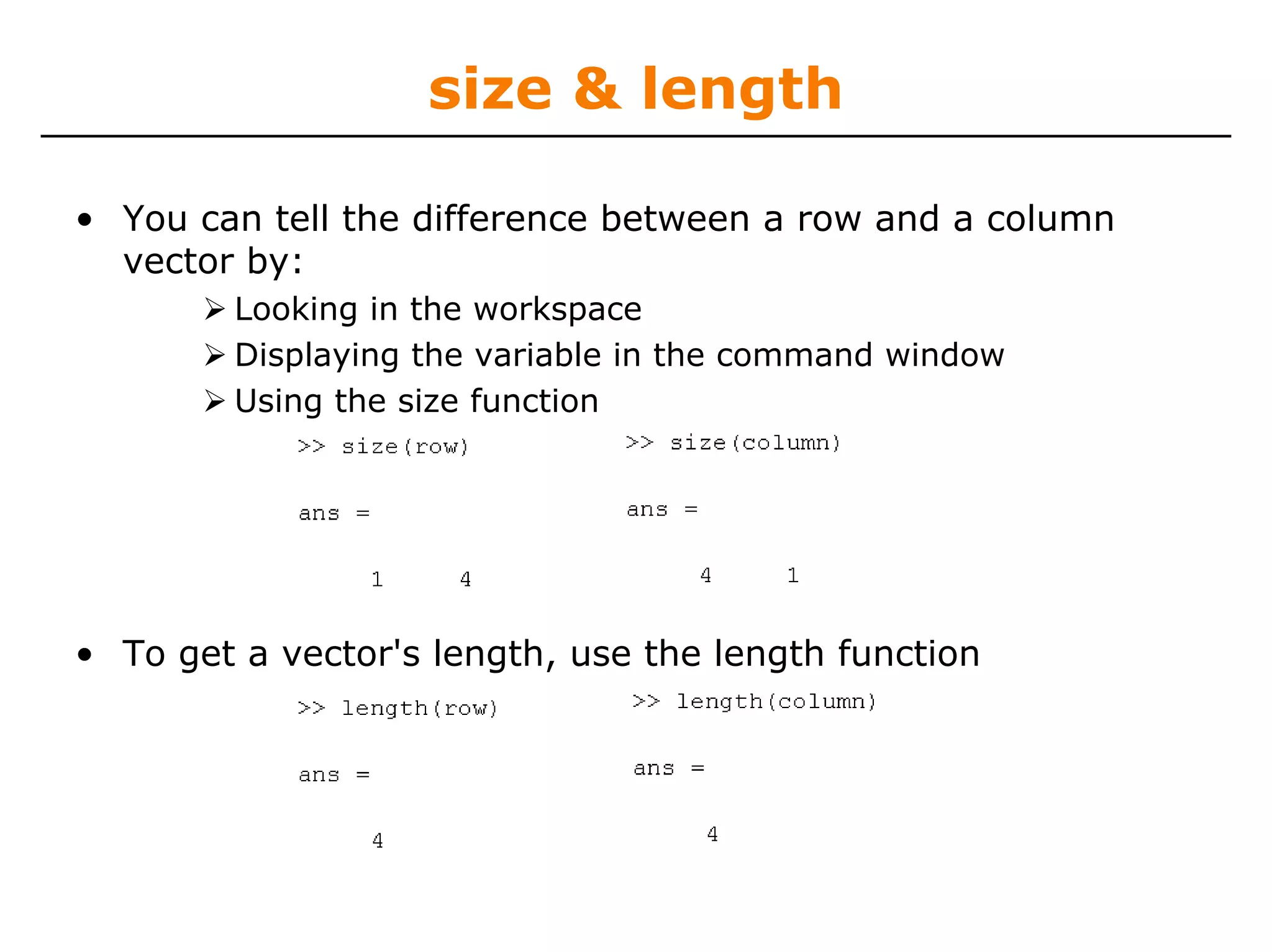
![Vector Indexing
• MATLAB indexing starts with 1, not 0
We will not respond to any emails where this is the
problem.
• a(n) returns the nth element
[13 5 9 10]
a(1) a(2) a(3) a(4)
• The index argument can be a vector. In this case, each
element is looked up individually, and returned as a vector
of the same size as the index vector.
» x=[12 13 5 8];
» a=x(2:3); a=[13 5];
» b=x(1:end-1); b=[12 13 5];](https://image.slidesharecdn.com/matlablec1-100301012417-phpapp02/75/Matlab-lec1-37-2048.jpg)
![Matrix Indexing
• Matrices can be indexed in two ways
using subscripts (row and column)
using linear indices (as if matrix is a vector)
• Matrix indexing: subscripts or linear indices
b(1,1) ⎡14 33⎤ b(1,2) b(1) ⎡14 33⎤ b(3)
b(2,1)
⎢9 8⎥ b(2,2) b(2)
⎢9 8⎥ b(4)
⎣ ⎦ ⎣ ⎦
• Picking submatrices
» A = rand(5) % shorthand for 5x5 matrix
» A(1:3,1:2) % specify contiguous submatrix
» A([1 5 3], [1 4]) % specify rows and columns](https://image.slidesharecdn.com/matlablec1-100301012417-phpapp02/75/Matlab-lec1-38-2048.jpg)
![Advanced Indexing 1
• The index argument can be a matrix. In this case, each
element is looked up individually, and returned as a matrix
of the same size as the index matrix.
» a=[-1 10 3 -2]; ⎡ −1 10 −2 ⎤
b=⎢ ⎥
» b=a([1 2 4;3 4 2]); ⎣ 3 −2 10 ⎦
• To select rows or columns of a matrix, use the :
⎡12 5 ⎤
c=⎢
⎣ −2 13⎥
⎦
» d=c(1,:); d=[12 5];
» e=c(:,2); e=[5;13];
» c(2,:)=[3 6]; %replaces second row of c](https://image.slidesharecdn.com/matlablec1-100301012417-phpapp02/75/Matlab-lec1-39-2048.jpg)
![Advanced Indexing 2
• MATLAB contains functions to help you find desired values
within a vector or matrix
» vec = [1 5 3 9 7]
• To get the minimum value and its index:
» [minVal,minInd] = min(vec);
• To get the maximum value and its index:
» [maxVal,maxInd] = max(vec);
• To find any the indices of specific values or ranges
» ind = find(vec == 9);
» ind = find(vec > 2 & vec < 6);
find expressions can be very complex, more on this later
• To convert between subscripts and indices, use ind2sub,
and sub2ind. Look up help to see how to use them.](https://image.slidesharecdn.com/matlablec1-100301012417-phpapp02/75/Matlab-lec1-40-2048.jpg)
![Exercise: Vector Indexing
• Evaluate a sine wave at 1,000 points between 0 and 2*pi.
• What’s the value at
Index 55
Indices 100 through 110
• Find the index of
the minimum value,
the maximum value, and
values between -0.001 and 0.001
» x = linspace(0,2*pi,1000);
» y=sin(x);
» y(55)
» y(100:110)
» [minVal,minInd]=min(y)
» [maxVal,maxInd]=max(y)
» inds=find(y>-0.001 & y<0.001)](https://image.slidesharecdn.com/matlablec1-100301012417-phpapp02/75/Matlab-lec1-41-2048.jpg)
![What does plot do?
• plot generates dots at each (x,y) pair and then connects the dots
with a line
• To make plot of a function look smoother, evaluate at more points
» x=linspace(0,4*pi,1000);
» plot(x,sin(x));
• x and y vectors must be same size or else you’ll get an error
» plot([1 2], [1 2 3])
error!!
1 1
10 x values: 0.8
0.6
1000 x values:
0.8
0.6
0.4 0.4
0.2 0.2
0 0
-0.2 -0.2
-0.4 -0.4
-0.6 -0.6
-0.8 -0.8
-1 -1
0 2 4 6 8 10 12 14 0 2 4 6 8 10 12 14](https://image.slidesharecdn.com/matlablec1-100301012417-phpapp02/75/Matlab-lec1-45-2048.jpg)
![Exercise: Plotting
• Plot f(x) = e^x*cos(x) on the interval x = [0 10]. Use a red
solid line with a suitable number of points to get a good
resolution.
» x=0:.01:10;
» plot(x,exp(x).*cos(x),’r’);](https://image.slidesharecdn.com/matlablec1-100301012417-phpapp02/75/Matlab-lec1-48-2048.jpg)

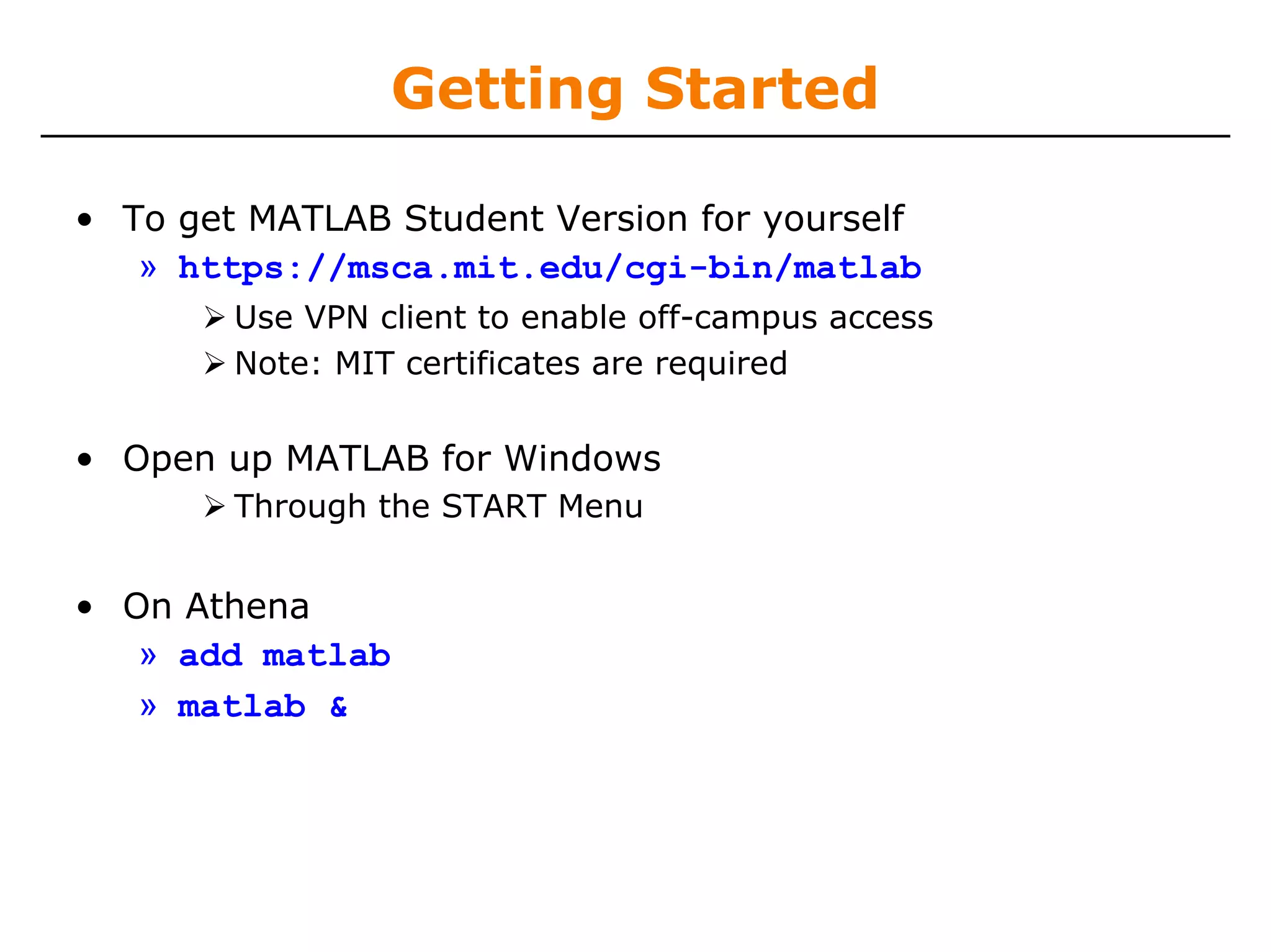
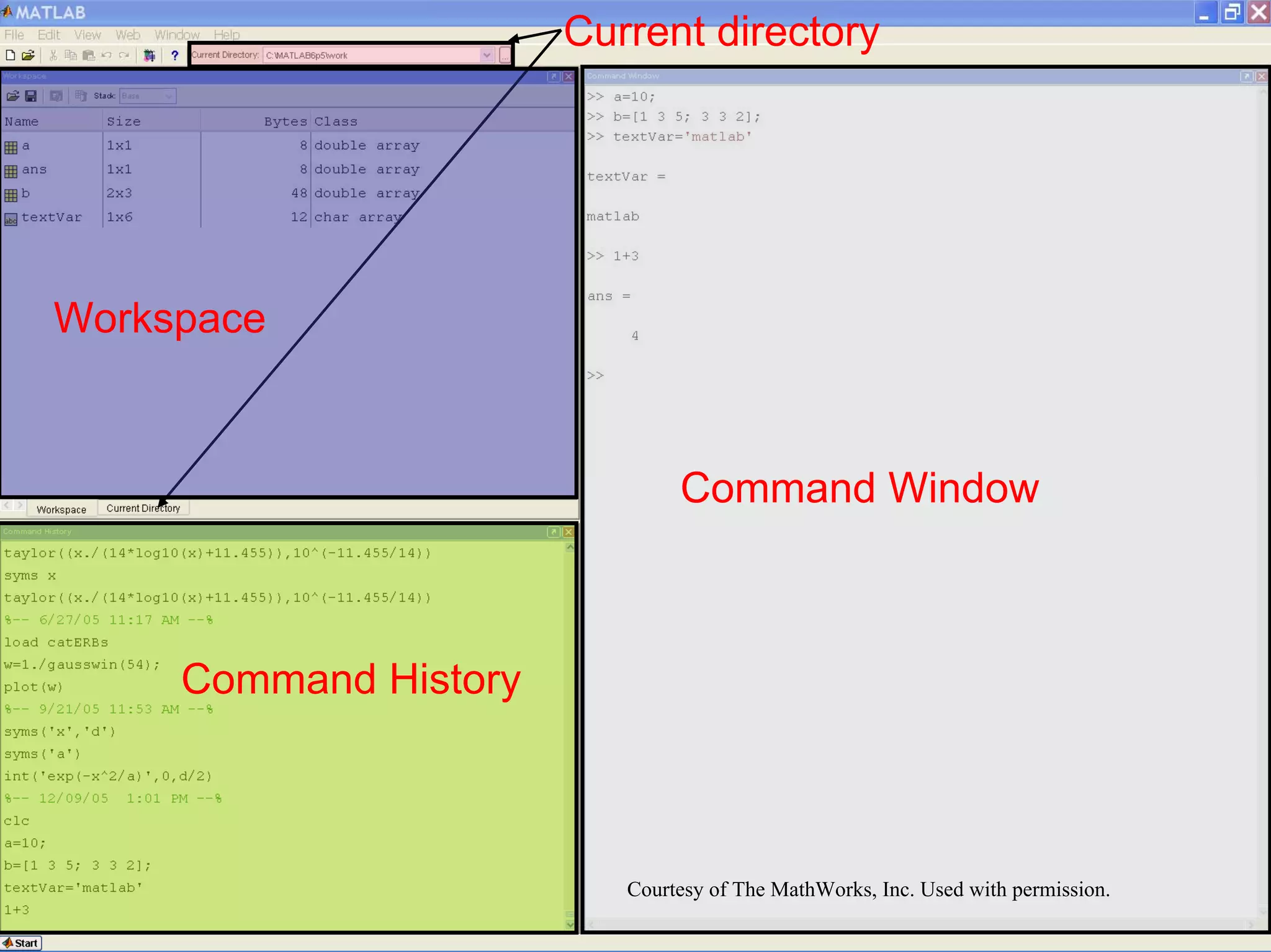
This document provides a summary of a course on introduction to MATLAB. The course includes 7 lectures covering topics like variables, operations, plotting, visualization, programming, solving equations and advanced methods. It will have problem sets to be submitted after each lecture and requirements to pass include attending all lectures and completing all problem sets. The course materials provide an overview of MATLAB including getting started, creating and manipulating variables, and basic plotting.


![Reduction of multiple subsystem [compatibility mode]](https://cdn.slidesharecdn.com/ss_thumbnails/reductionofmultiplesubsystemcompatibilitymode-110418075355-phpapp01-thumbnail.jpg?width=640&height=640&fit=bounds)