Downloaded 10 times
![Arrays
• Matlab = Matrix Laboratory, so do things with matrices!
• Create your first matrix!
• a = [1234], Row Vector!
• Indexing in matlab begins with 1 (NOT 0)
• Add more rows: a = [1234; 2345; 3456]
• Note This also works: a = [1, 2, 3, 4; 2, 3, 4, 5; 3, 4, 5, 6]
• We can call values from this array:
• a(1, 2)
• 2
• Or assign a value to a particular position:
• a(1, 2) = 10
• The notation is (row, column)](https://image.slidesharecdn.com/matlabpt1-150626144431-lva1-app6891/75/Matlab-pt1-6-2048.jpg)
![Array Operations
• Colon operator:
• a = [123; 234; 456]
• The colon denotes start:end. Note: if you just place a
colon it will select everything.
• Select the first two rows of our matrix:
• a(1 : 2, :)
• What does a(1, :) do?
• We can also add to each element of the array:
• a − a
• a − 10
• We can do traditional and element wise multiplication of
matrices:
• traditional: a ∗ a, element wise: a. ∗ a
• In a similar way you can do other things element wise to a
matrix ex.: a. ∧ 3](https://image.slidesharecdn.com/matlabpt1-150626144431-lva1-app6891/75/Matlab-pt1-8-2048.jpg)
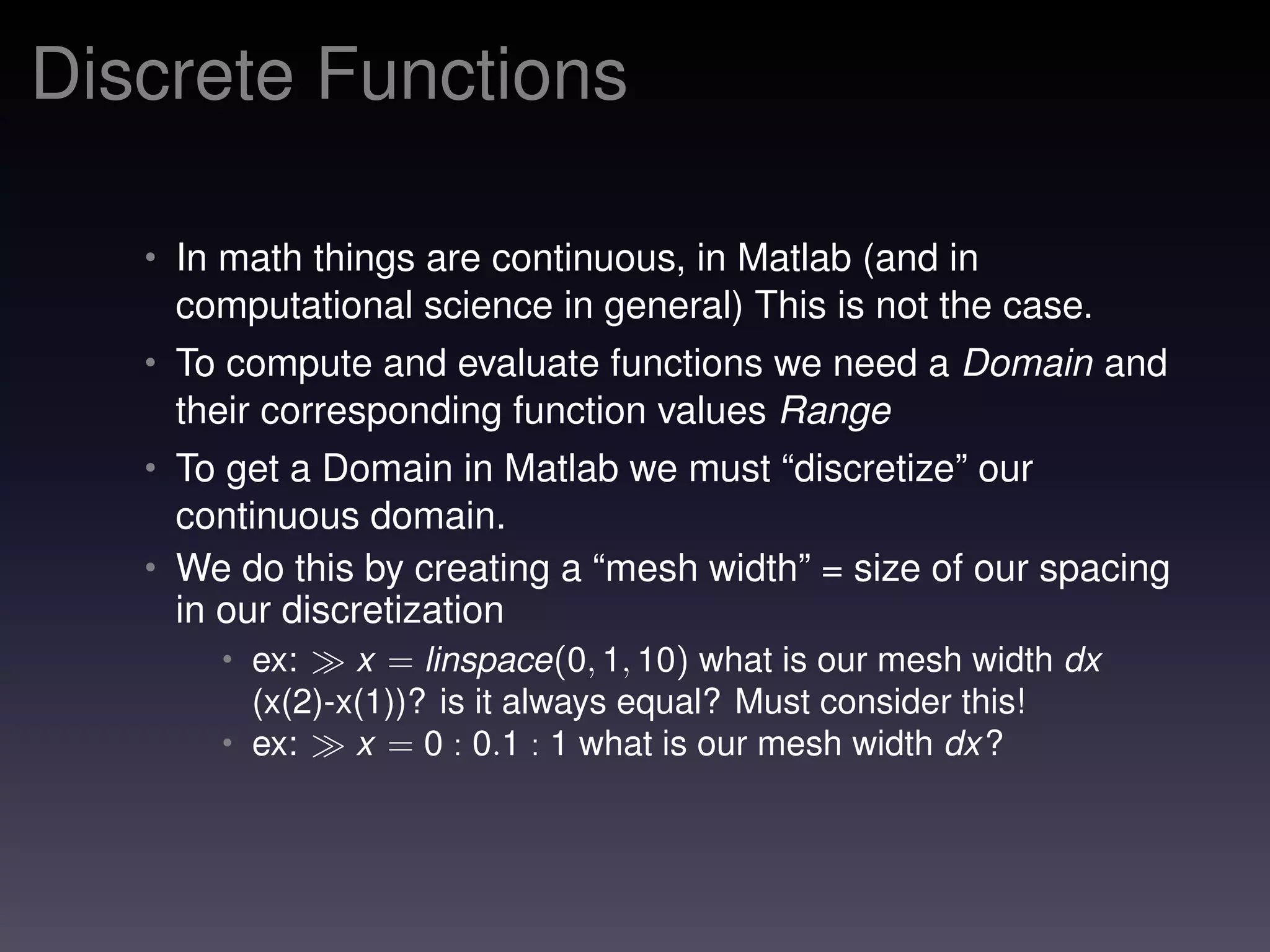
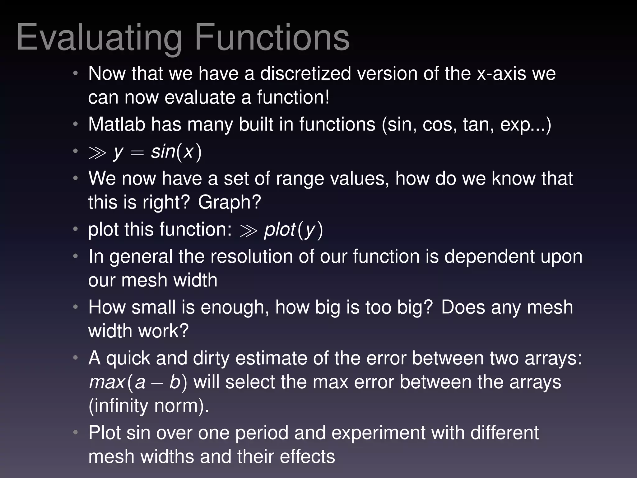

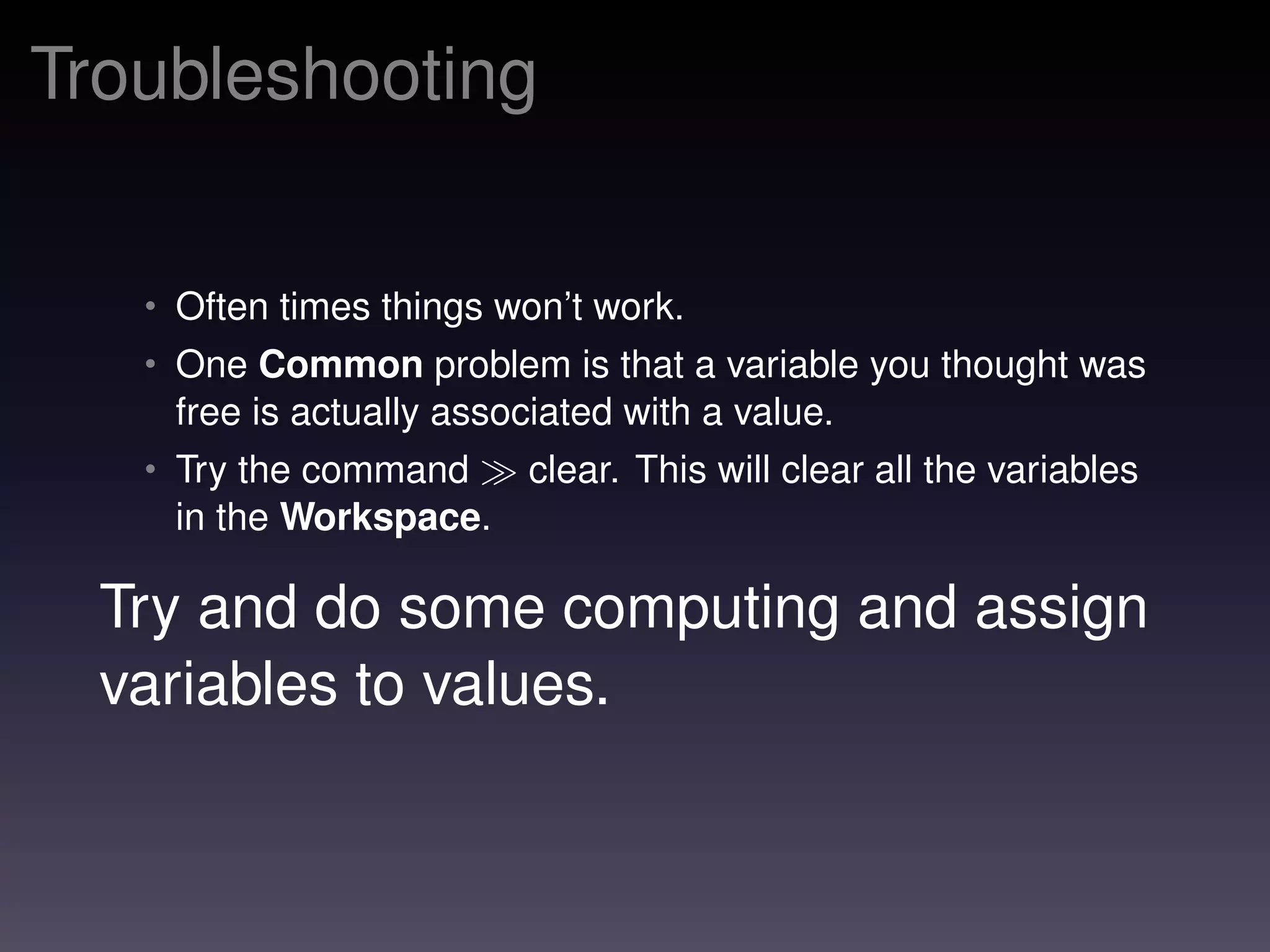
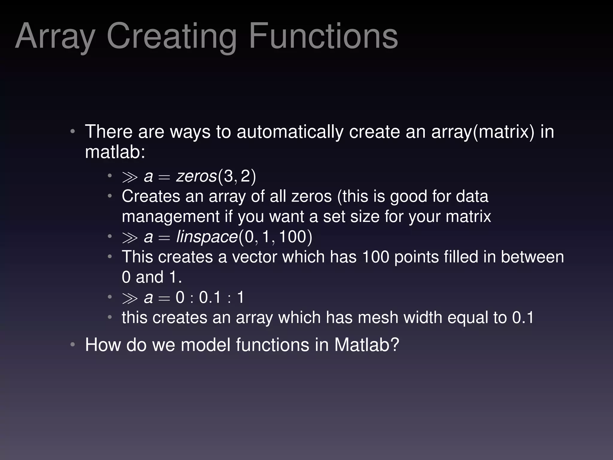
The document is a set of MATLAB notes that introduces its basic desktop environment, arithmetic operations, and matrix handling. It covers key concepts such as creating matrices, using built-in functions, and evaluating functions with discretization. Additionally, it presents troubleshooting tips, array operations, and outlines an assignment involving plotting a function.


![[DSC Europe 25] Nikola Rajovic - Hardware Technologies Under the Hood: RISC-V...](https://cdn.slidesharecdn.com/ss_thumbnails/o2gptrmtoyqndgoshwgq-dsc2025-tenstorrent-rajovic-251205090438-814685f5-thumbnail.jpg?width=640&height=640&fit=bounds)


![[DSC Europe 25] Bassam Maharmeh - Artificial Intelligence: Opportunities and ...](https://cdn.slidesharecdn.com/ss_thumbnails/thhfmr2fqpawzj7hsjpg-5-251211083048-2c23204f-thumbnail.jpg?width=640&height=640&fit=bounds)
![[DSC Europe 25] Jovan Bogicevic - Legacy to AI-Driven Defense: Transforming D...](https://cdn.slidesharecdn.com/ss_thumbnails/rsarluadt563hntyfc8q-3-251211083849-3e7bc4c0-thumbnail.jpg?width=640&height=640&fit=bounds)

![[DSC Europe 25] Dusan Pavlov - There Is No Spoon: Inferring Vision from Neura...](https://cdn.slidesharecdn.com/ss_thumbnails/wg0v1umoqjm4nnbd3p0v-there-is-no-spoon-251205085715-6d81d6c5-thumbnail.jpg?width=640&height=640&fit=bounds)

![[DSC Europe 25] Aleksandra Dragicevic - AI-Boosted Research in Healthcare: Fr...](https://cdn.slidesharecdn.com/ss_thumbnails/iqwngszurf2r7pi1lnnj-4-aleksandra-dragicevic-ad-dsc-europe-conference-20-251208151905-37c3238a-thumbnail.jpg?width=640&height=640&fit=bounds)
![[DSC Europe 25] Goran Obradovic - The Rise of Sovereign AI: Building the Regi...](https://cdn.slidesharecdn.com/ss_thumbnails/7nw2xxixrxqdxvrb5wca-6-251205085714-ab09a2ac-thumbnail.jpg?width=640&height=640&fit=bounds)
![[DSC Europe 25] Dragan Vucic - Building the Learning Organization - How AI Tr...](https://cdn.slidesharecdn.com/ss_thumbnails/8brigo2sbu6qur6gxrra-7-251205085715-6ae07d24-thumbnail.jpg?width=640&height=640&fit=bounds)
![[DSC Europe 25] Milan Sekuloski - Data, Defence, and Development: Cybersecuri...](https://cdn.slidesharecdn.com/ss_thumbnails/dfrkwwx4qly6atqpbl4z-4-251209104645-c3d4b0ca-thumbnail.jpg?width=640&height=640&fit=bounds)

![[DSC Europe 25] Max Talanov - Non digital NNs.pptx](https://cdn.slidesharecdn.com/ss_thumbnails/wif8tr3gtua74qvtopke-non-digital-nns-251205090438-26b0eea6-thumbnail.jpg?width=640&height=640&fit=bounds)
![[DSC Europe 25] Sara Polak - The Archaeology of Innovation: AI as the Next Cr...](https://cdn.slidesharecdn.com/ss_thumbnails/7ecbscdnt8mlcuqbd2ln-2-sara-polak-ai-creative-industries-251208152533-aa1fcf54-thumbnail.jpg?width=640&height=640&fit=bounds)

