This document provides an overview and table of contents for a textbook on control systems by Dr. N.C. Jagan. The textbook covers various topics related to modeling, analysis, and design of control systems, including mathematical modeling of physical systems, time response analysis, stability analysis using Routh-Hurwitz and root locus methods, frequency response analysis using Bode and Nyquist plots, and closed loop control design. It contains 7 chapters and provides problems at the end of each chapter. The textbook is copyrighted and published by BSP BS Publications in Hyderabad, India.

2. Control Systems
Second Edition
Dr. N.C. Jagan
B.E., ME., Ph.D., MlSTE, FIE
Retd. Professorin Electrical Engineering
University College of Engineering
Osmania University, Hyderabad.
BSP BS Publications
4-4-309, Giriraj Lane, Sultan Bazar,
Hyderabad - 500 095 - A.P.
Phone: 040-23445605,23445688

3. Copyright © 2008 by Publisher
All rights reserved
No part of this book or parts thereof may be reproduced, stored in a retrieval system or
transmitted in any language or by any means, electronic, mechanical, photocopying,
recording or otherwise without the prior written permission of the publishers.
Published by :
SSP BS Publications
Printed at
4-4-309, Giriraj Lane, Sultan Bazar,
Hyderabad - 500 095 - A.P.
Phone: 040-23445605,23445688
e-mail: contactus@bspublications.net
www.bspublications.net
Adithya Art Printers
Hyderabad
ISBN: 978-81-7800-177-2 (HB)

4. Contents
1 Introduction 1
1.1 Why Automatic Control ? .................................................................... 1
1.2 Open Loop and Closed Loop Control Systems ................................ 2
1.3 Open Loop Vs Closed Loop Control Systems ................................... 3
1.4 Feedback Control Systems ................................................................ 4
1.5 Classification of Control Systems ...................................................... 4
1.5.1 Continuous Time Feedback Control Systems ..................... 5
1.5.2 Discrete Data Feedback Control Systems .......................... 5
1.5.3 Linear Control Systems ........................................................ 6
1.5.4 Non-Linear Control Systems ................................................ 6
2 Mathematical Modelling ofPhysical Systems 8
2.1 Introduction .............................................................,........................... 8
2.2 Mathematical Models of Physical Systems ........................................ 8
2.2.1 Electrical Systems ................................................................. 9
2.2.2 Dual Networks ..................................................................... 14
2.2.3 Mechanical Systems ........................................................... 15
2.2.4 Analogous Systems ............................................................ 18
2.2.5 Gears ................................................................................... 24
2.2.6 Thermal Systems ................................................................ 27
2.2.7 Fluid Systems ...................................................................... 29

5. Contents
2.3 Block Diagrams of Closed Loop Syst~ms ........................................ 34
2.3.1 Block Diagram Reduction Techniques ............................... 35
2.4 Signal Flow Graph Representation of Control Systems ................. 42
2.4.1 Construction of a Signal Flow Graph for a System ........... 43
2.4.2 Mason's Gain Formula ....................................................... 44
2.5 Effects of Feedback ......................................................................... 52
2.5.1 Effect on system dynamics ................................................. 53
2.5.2 Effect due to parameter variations .................................... 54
2.5.3 Effect on Bandwidth ............................................................ 57
2.5.4 Effect on Noise Signals ....................................................... 58
2.6 Modelling of Elements of Control Systems ...................................... 59
2.6.1 DC Servo Motor .................................................................. 59
2.6.2 AC Servo Motors ................................................................. 63
2.6.3 Synchros ............................................................................. 65
2.6.4 AC Tacho Generator ........................................................... 68
2.6.5 DC Tacho Generator .......................................................... 69
2.6.6 Potentiometers .................................................................... 69
2.6.7 Stepper Motors ................................................................... 71
Problems ........................................................................................~............ 73
3 Time Response Analysis ofControl Systems 81
3.1 Introduction ....................................................................................... 81
3.2 Standard Test Signals ....................................................................... 81
3.2.1 Impulse Signal ....................................................................... 81
3.2.2 Step Signal ........................................................................... 82
3.2.3 Ramp signal .......................................................................... 82
3.2.4 Parabolic signal .................................................................... 82
3.3 Representation of Systems .............................................................. 83
3.4 First Order System ........................................................................... 85
3.4.1 Response to a Unit Step Input ............................................. 85
3.4.2 Response to a Unit Ramp Input or Unit Velocity Input ........ 86
3.4.3 Response to a Unit Parabolic or Acceleration Input ............ 87
3.5 Second Order System ...................................................................... 88
3.5.1 Response to a Unit Step Input ............................................. 88
3.5.2 Response to a Unit Ramp Input ........................................... 92
3.5.3 Time Domain Specifications of a Second Order System ..... 93

6. Contents
3.6 Steady State Errors .......................................................................... 99
3.6.1 Error Constants .................................................................... 99
3.6.2 Dependence of Steadystate Error on Type of the System 101
3.6.3 Generalized Error Coefficients - Error Series .................... 104
3.7 Design Specifications of a Control System .................................... 113
3.7.1 Proportional Derivative Error Control (PD control) ........... 114
3.7.2 Proportional Integral Controller (PI Control) ...................... 115
3.7.3 Proportional, Integral and Derivative Controller
(PID Control) ....................................................................... 116
3.7.4 Derivative Output Control ................................................... 116
Problems ...................................................................................................125
4 Stability of Systems 129
4.1 Introduction ..................................................................................... 129
4.2 Stability Preliminaries ...................................................................... 130
4.3 Necessary Conditions for Stability ................................................. 133
4.4 Routh - Hurwitz Stability Criterion ................................................... 134
4.5 Special Cases ................................................................................. 137
4.6 Relative Stability ............................................................................. 147
Problems ...................................................................................................149
5 Root LocusAnalysis 151
5.1 Introduction ..................................................................................... 151
5.2 Basic Idea ....................................................................................... 151
5.3 Development of Root Locus Technique ........................................ 153
5.4 Properties of Root Locus ............................................................... 155
Problems ...................................................................................................187
6 Frequency Response ofControl Systems, 190
6.1 Introduction ..................................................................................... 190
6.2 Time Domain AnalysiS Vs Frequency Domain Analysis ................ 190
6.3 Frequency Response of a Control System ................................... 191
6.4 Correlation Between Time Response and
Frequency Response ..................................................................... 194

7. Contents
6.5 Graphical Representation of Transfer Functions ......................... 196
6.5.1 Bode plots .......................................................................... 196
6.5,2 Polar Plots .......................................................................... 218
6.5.3 Log Magnitude Vs Phase Plots ......................................... 222
6.6 All Pass Systems ............................................................................ 223
6.7 Minimum Phase Systems ................................................................ 224
Problems ................................................................................................... 226
7 Nyquist Stability Criterion and
Closed Loop Frequency Response
229
7.1 Introduction ..................................................................................... 229
7.2 Principle of Argument ..................................................................... 230
7.3 Development of Nyquist Criterion .................................................. 234
7.3.1 Nyquist Contour ................................................................. 234
7.3.2 Nyquist Stability Criterion ........................" ......................... 234
7.3.3 Nyquist Contour When Open Loop Poles Occur
on jro-axis ............................................................................ 236
7.3.4 Nyquist Stability Criterion for Systems which are
Open Loop Stable .............................................................. 252
7.4 Relative Stability ............................................................................ 254
7.4.1 Measures of Relative Stability: Gain Margin .................... 256
7.4.2 Phase Margin ..................................................................... 257
7.4.3 Adjustment of Gain K for Desired Values of Gain and
Phase Margins Using Polar Plots ...................................... 260
7.4.4 Gain Margin and Phase Margin Using Bode Plot ............. 261
7.5 Closed Loop Frequency Response .............................................. 264
7.5.1 Constant M Circles ............................................................ 267
7.5.2 Constant N circles .............................................................. 269
7.5.3 Nichols Charts .................................................................... 272
Problems ...................................................................................................277
8 Design in Frequency Domain 281
8.1 Preliminaries of Design .................................................................. 281
8.2 A Design Example ...........................................................................282
8.3 Realisation of Compensators and their Characteristics ............... 285

8. Contents
8.3.1 Lead Compensator ............................................................ 286
8.3.2 Lag Compensator .............................................................. 290
8.3.3 Lag-Lead Compensator .................................................... 291
8.4 Cascade Compensation in Frequency Domain Using
Bode Plots ...................................................................................... 293
8.4.1 Design of Lead Compensator ........................................... 293
8.4.2 Design of Lag Compensator ............................................. 304
8.4.3 Design of Lag-Lead Compensator ................................... 311
Problems ................................................................................................... 316
9 State Space Analysis of Control Systems 318
9.1 Introduction .....................................................................................318
9.2 State Variables ................................................................................ 319
9.3 State Equations for Linear Systems .............................................. 321
9.4 Canonical Forms of State Models of Linear Systems ................... 324
9.4.1 Phase Variable Form ......................................................... 324
9.4.2 Diagonal Form ................................................................... 330
9.5 Transfer Function from State Model ............................................. 334
9.6 Diagonalisation .............................................................................. 337
9.6.1 Eigenvalues and Eigenvectors ......................................... 337
9.7 Solution of State Equation ............................................................. 345
9.7.1 Properties of State Transition Matrix ................................. 346
9.7.2 Methods of Computing State Transition Matrix ................. 346
9.8 Qualitative Analysis of Control Systems ....................................... 358
9.8.1 State Controllability ............................................................ 358
9.8.2 Observability ...................................................................... 366
9.8.3 Duality Principle ................................................................. 372
Problems ................................................................................................... 373
Answers to Problems ............................................................................. 377
MCQ's from Competitive Examinations ............................................. 387
Answers to MCQ's ..................................................................................481
-djJ-

9. "This page is Intentionally Left Blank"

10. 1 Introduction
1.1 Why Automatic Control ?
Automatic control of many day to day tasks relieves the human beings from performing repetitive
manual operations. Automatic control allows optimal performance ,of dynamic systems, increases
productivity enormously, removes drudgery ofperforming same task again and again. Imagine manual
control of a simple room heating system. If the room temperature is to be maintained at a desired
temperature TOe, by controlling the current in an electrical heating system, the current may be
adjusted by moving the variable arm in a rheostat. The temperature ofthe room depends on a host of
factors : number of persons in the room, the opening and closing of doors due to persons moving in
and out, fluctuation ~n the supply voltage etc. A human operator has to continuously monitor the
temperature indicated by a thermometer and keep on adjusting the rheostat to maintain the temperature
all the twenty four hours. The operator should be continuously alert and relentlessly perform a simple
job ofmoving the arm ofthe rheostat. Any mistake on his part may result in great discomfiture to the
persons in the room.
Now, imagine the same operation of measuring the temperature, estimating the error between
the desired temperature and the actual temperature, moving the arm ofthe rheostat accurately by
an automatic controller. Since error.between the actual temperature and the desired temperature
is continuously obtained and used to activate the controller, any disturbances caused due to
movements of persons occupying the room, supply variations etc. will be automatically taken
care of. How much of a relief it is ! This is only a simple task, but many complex industrial
processes, space craft systems, missile guidance systems, robotic systems, numerical control
of machine tools employ automatic control systems. There is no field in engineering where
automatic control is not employed. Even human system is a very complex automatic feedback
control system. The modem engineers and scientists must, therefore, have a thorough knowledge
of the principles of automatic control systems.

11. 2 Control Systems
The first automatic control was invented by James Watt. He employed a centrifugal or fly ball
governor for the speed control of a steam engine in 1770. But much of the advances had to wait for
more than a hundred years, until Minorsky, Hazen and Nyquist contributed significantly in the
development ofcontrol system theory. Hazen coined the word "servo mechanisms" to describe feedback
control systems in which the variable to be controlled is a mechanical position, velocity or acceleration
ofa given object. During 1940s, frequency response methods and root 'locus techniques were developed
to design linear, stable, closed loop control systems with given performance measures. In later part
of 1950s, much emphasis was given in designing systems, which not only satisfied given performance
measures, but also provided optimum design in a given sense. As the systems became more and more
complex with more number of inputs and outputs and with the advent of digital computers, modern
control theory r~lerted back to methods based on time domain analysis and synthesis using state
variable representations.
In the period between 1960 and 1980, to cope up with the complexity and stringent requirements
on accuracy, speed and cost adaptive control was developed. Both deterministic and stochastic systems
were considered and controllers were designed which were optimal, adaptive and robust. The principles
developed in automatic control theory were not only used in engineering applications, but also in non
engineering systems like economic, socio economic systems and biological systems.
1.2 Open Loop and Closed Loop Control Systems
Open Loop Control Systems: A system in which the output has no effect on the control action is
known as an open loop control system. For a given input the system produces a certain output. If
there are any disturbances, the out put changes and there is no adjustment of the input to bring back
the output to the original value. A perfect calibration is required to get good accuracy and the system
should be free from any external disturbances. No measurements are made at the output.
A traffic control system is a good example of an open loop system. The signals change according
to a preset time and are not affected by the density of traffic on any road. A washing machine is
another example of an open loop control system. The quality of wash is not measured; every cycle
like wash, rinse and dry' cycle goes according to a preset timing.
Closed Loop Control Systems: These are also known as feedback control systems. A system which
maintains a prescribed relationship between the controlled variable and the reference input, and uses
the difference between them as a signal to activate the control, is known as a feedback control
system. The output or the controlled variable is measured and compared with the reference input and
an error signal is generated. This is the activating signal to the controller which, by its action, tries to
reduce the error. Thus the controlled variable is continuously fedback and compared with the input
signal. If the error is reduced to zero, the output is the desired output and is equal to the reference
input signal.

12. Introduction 3
1.3 Open Loop Vs Closed Loop Control Systems
The open loop systems are simple and easier to build. Stability, which will be discussed in later
chapters, is not a problem. Open loop systems are cheaper and they should be preferred whenever
there is a fixed relationship between the input and the output and there are no disturbances. Accuracy
is not critical in such systems.
Closed loop systems are more complex, use more number ofelements to build and are costly. The
stability is a major concern for closed loop systems. We have to ensure that the system is stable and
will not cause undesirable oscillations in the output. The major advantage of closed loop system is
that it is insensitive to external disturbances and variations in parameters. Comparatively cheaper
components can be used to build these systems, as accuracy and tolerance do not affect the
performance. Maintenance of closed loop systems is more difficult than open loop systems. Overall
gain of the system is also reduced.
Open Loop Systems
Advantages
1. They are simple and easy to build.
2. They are cheaper, as they use less number of components to build.
3. They are usually stable.
4. Maintenance is easy.
Disadvantages
1. They are less accurate.
2. If external disturbances are present, output differs significantly from the desired value.
3. If there are variations in the parameters of the system, the output changes.
Closed Loop Systems
Advantages
1. They are more accurate.
2. The effect of external disturbance signals can be made very small.
3. The variations in parameters of the system do not affect the output of the system i.e. the
output may be made less sensitive to variation is parameters. Hence forward path components
can be of less precision. This reduces the cost of the system.
4. Speed of the response can be greatly increased.
Disadvantages
1. They are more complex and expensive
2. They require higher forward path gains.
3. The systems are prone to instability. Oscillations in the output many occur.
4. Cost of maintenance is high.

13. 4 Control Systems
1.4 Feedback Control Systems
Fig. 1.1 represents a feedback control system.
Controller
Reference
input
r------------,
I + e(t)
------~~ ~--------~
or r(t) I -
Command I
signal
error or
actuating I
signal_ _ _ _ _ _ _ _ _ --1
Feedback b(t)
signal
Fig. 1.1 A feedback control system
Manipulating signal
Controlled output
c(t)
A feedback control system is represented as an interconnection of blocks characterized by an
input output relation. This method of representing a control system is known as a block diagram
representation. While other methods are also used to represent the control system, this is more
popular. The input to the entire system is called as a reference input or a command input, ret).
An error detector senses the difference between the reference input and the feedback signal equal to
or proportional to the controlled output. The feedback elements measure the controlled output and
convert or transfonn it to a suitable value so that it can be compared with the reference input. If the
feedback signal, bet), is equal to the controlled output, c(t), the feedback system is called as unity
feedback system.
The difference between the reference input and the feedback signal is known as the error signal or
actuating signal e(t), This signal is the input to the control elements which produce a signal known as
manipulated variable, u(t). This signal manipulates the system or plant dynamics so that the desired
output is obtained. The controller acts until the error between the output variable and the reference
input is zero. If the feedback path is absent, the system becomes an open loop control system and is
represented in Fig. 1.2.
Input I I u(t) ~I Plant IOutpu.:. c(t)
r(t) ----I.~ Controller .... . ...
Fig. 1.2 Open loop control system
1.5 Classification of Control Systems
Depending on the type of signals present at the various parts of a feedback control system, the
system may be classified as a (i) continuous time feedback control system or a (ii) discrete time
feedback control system.

14. Introduction 5
1.5.1 Continuous Time Feedback Control Systems
Ifthe signals in all parts ofa control system are continuous functions oftime, the system is classified
as continuous time feedback control system. Typically all control signals are of low frequency and if
these signals are unmodulated, the system is known as a d.c. control system. These systems use
potentiometers as error detectors, d.c amplifiers to amplify the error signal, d.c. servo motor as
actuating device and d.c tachometers or potentiometers as feedback elements. If the control signal is
modulated by an a.c carrier wave, the resulting system is usually referred to as an a.c control system.
These systems frequently use synchros as error detectors and modulators oferror signal, a.c amplifiers
to amplify the error signal and a.c servo motors as actuators. These motors also serve as demodulators
and produce an unmodulated output signal.
1.5.2 Discrete Data Feedback Control Systems
Discrete data control systems are those systems in which at one or more pans of the feedback
control system, the signal is in the form of pulses. Usually, the error in such system is sampled at
uniform rate and the resulting pulses are fed to the control system. In most sampled data control
systems, the signal is reconstructed as a continuous signal, using a device called 'hold device'. Holds
of different orders are employed, but the most common hold device is a zero order hold. It holds the
signal value constant, at a value equal to the amplitude of the input time function at that sampling
instant, until the next sampling instant. A typical discrete data control system is shown in Fig. 1.3
which uses a sampler and a data hold.
ret) c(t)
Sampler
Fig. 1.3 Discrete data control system
These systems are also known as sampled data control systems.
Discreet data control systems, in which a digital computer is used as one ofthe elements, are
known as digital control systems. The input and output to the digital computer must be binary numbers
and hence these systems require the use ofdigital to analog and analog to digital converters. A typical
digital control system is shown in Fig. 1.4.
c(t)
Fig. 1.4 Digital feedback control system
Digital devices may be employed in the feedback circuits as measuring elements.

15. 6 Control Systems
A further classification of control systems can be made depending on the nature of the systems,
namely,
1. Linear control systems
2. Non-linear control systems
1.5.3 Linear Control Systems
If a system obeys superposition principle, the system is said to be a linear system. Let xl(t) and x2(t)
be two inputs to a system and Yl(t) and Yit) be the corresponding outputs. For arbitrary real constants
kl and~, and for input kl xl(t) + ~ x2(t), if the output of the system is given by kl Yl(t) + k2 Y2(t),
then the system is said to be a linear system. There are several simple techniques available for the
analysis and design of linear control systems.
1.5.4 Non-Linear Control Systems
Any system which does not obey superposition principle is said to be a non-linear system. Physical
systems are in general non-lienar and analysis of such systems is very complicated. Hence these
systems are usually linearlised and well known linear techniques are used to analyse them.
These systems can be further classified depending on whether the parameters of the system are
constants, or varying with respect to time. When the input to a system is delayed by T seconds, ifthe
output is also delayed by the same time T, the system is said to be a time invariant system. Thus
x(t) __..J~~ System 1----..y(t) x (t- T) ----.!~ System 1----..Y (t-' T)
(a) (b)
Fig. 1.5 Time invariant system.
On the other hand, ifthe output is dependent on the time ofapplication ofthe input, the system is
said to be a time varying system. Like non-linear systems, time varying systems also are more
complicated for analysis. In this text we will be dealing with linear time invariant continuous systems
only.
The layout ofthis book is asfollows:
The mathematical modelling of processes suitable for analysis and design of controllers is discussed
in Chapter 2. Typical examples from electrical, mechanical, pneumatic and hydraulic systems are
given. The transfer function ofthe overall system is obtained by block diagram and signal flow graph
representation of the systems. The effects of feedback on the performance of the system are also
discussed. .
In chapter 3, time domain specifications of the control system are defined with respect to the
response ofa typical second order system, for unit step input. Steady state errors are defined and the
use ofPID controllers is discussed to satisfy the design specifications of a control system. In chapter
4, the stability aspects of the system are discussed and algebraic criteria for obtaining the stability of
the system are developed.

16. Introduction 7
The roots of the characteristic equation of the system determine the behaviour and stability of a
control system. The roots change as the parameters are changed. The concept of the locus of these
roots as one ofthe parameters, usually the gain ofthe amplifier, is changed from 0 to 00 is discussed
in chapter 5. The design of a control system is rendered very easy by considering the response ofthe
system to sinusoidal signals. Frequency domain analysis and development of frequency domain
specifications are discussed in chapter 6.
Relative stability aspects are considered in chapter 7. Nyquist stability criterion is developed and
measures of relative stability, viz, gain margin on phase margin are dermed.
In chapter 8, design ofcompensating RC networks to satisfy the design specifications ofa control
system in frequency domain is discussed. In chapter 9, state space representation of control systems
is developed, which enables modern techniques to be used in the design of control systems.
-~-

17. 2 Mathematical Modelling of
Physical Systems
2.1 Introduction
Whenever a task is to be performed, a set of physical objects are connected together and a suitable
input is given to them, to obtain the desired output. This group of objects is usually termed as the
'system'. The system may consist of physical objects and it may contain components, biological
economical or managerial in nature. In order to analyse, design or synthesise a complex system, a
physical model has to be obtained. This physical model may be a simplified version of the more
complex system. Certain assumptions are made to describe the nature of the system. Usually all
physical systems in the world are nonlinear in nature. But under certain conditions these systems may
be approximated by linear systems. Hence for certain purposes, a linear model may be adequate. But
if stringent accuracy conditions are to be satisfied, linear model may not be suitable. Similarly, the
parameters ofthe system may be functions oftime. But if they are varying very slowly, they may be
assumed to be constant. In many engineering systems the elements are considered to be lumped and
their behaviour is described by considering the effect at its end points called terminals. Long lines
transmitting electrical signals, may not be adequately represented by lumped elements. A distributed
parameter representation may be called for in this case. Hence depending on the requirements of a
given job, suitable assumptions have to be made and a 'physical model' has to be first defined. The
behaviour of this physical model is then described in terms of a mathematica~ model so that known
techniques of mathematical analysis can be applied to the given system.
2.2 Mathematical Models of Physical Systems
The system may be considered to be consisting of an inter connection of smaller components or
elements, whose behaviour can be described by means of mathematical equations or relationships.
In this book, we will be considering systems made up of elements which are linear, lumped and
time invariant. An element is said to be linear if it obeys the principle of super position
and homogeneity. If the responses of the element for inputs xj(t) and xit) are Yj(t) and Yit)
respectively, the element is linear ifthe response to the input, kj xj(t) + Is xit) is kj Yj(t) + Is Y2(t)
as shown in Fig. 2.1.

18. Mathematical Modelling of Physical Systems 9
x,(t) I• • LInear element
Fig. 2.1 Definition of linear element
An element is said to be 'lumped' ifthe physical dimensions or spacial distribution ofthe element
does not alter the signal passing through it. The behaviour ofsuch elements are adequately represented
by the effects at the end points called terminals. The temperature of a body may be treated as same,
at all points ofthe body under certain conditions. Similarly the mass of a body may be considered as
concentrated at a point. A rotating shaft may be considered as rigid. An electrical resistor may be
represented by a lumped element, since the current entering at one terminal leaves the other terminal
without undergoing any change. The voltage distribution in the physical body of the resistor is not
considered. Only the voltage across its terminals is taken for analysis. These are some examples of
lumped elements.
If the parameters representing the elements are not changing with respect to time, the element is
said to be time invariant. Thus if a system is composed of linear, lumped and time invariant
elements, its behaviour can be modelled by either linear algebraic equations or linear differential
equations with constant coefficients. If the input output relations are algebraic, the system is said to
be a static system. On the other hand, if the relations are described by differential equations, the
system is said to be a dynamic system. We are mostly concerned with dynamic response of the
systems and therefore, one ofthe ways by which a system is mathematically modelled is by differential
equations. Another most useful and common mathematical model is the Transfer function' of the
system. It is defined as the ratio of Laplace transform of the output to the Laplace transform of the
input. This is illustrated in Fig. 2.2.
R (s) .LI__T_(_S)_---If---
C
-(.!)
Fig. 2.2 Transfer function of a system
In Fig. 2.2, the transfer function is,
C(s)
T(s) = R(s) .....(2.1)
In defining the transfer function, it is assumed that all initial conditions in the system are zero.
Having defined the two common ways of describing linear systems, let us obtain the
mathematical models ofsome commonly occuring Electrical, Mechanical, Thermal, Fluid, Hydraulic
systems etc.
2.2.1 Electrical Systems
Most of the electrical systems can be modelled by three basic elements : Resistor, inductor, and
capacitor. Circuits consisting of these three elements are analysed by using Kirchhoff's Voltage law
and Current law.

19. 10
(a) Resistor: The circuit model of resistor is shown in Fig. 2.3 (a)
i(t) R
?~.WJ.Nv-~
~~----- v(t) ----~J
Fig. 2.3(a) Circuit model of resistor
The mathematical model is given by the Ohm's law relationship,
vet) = i(t) R; i(t) = vet)
R
(b) Inductor: The circuit representation is shown in Fig. 2.3 (b)
Fig. 2.3(b) Circuit model of inductor
The input output relations are given by Faraday's law,
or
( )
- L diet)vt - --
dt
I
i(t) = - Jvdt
L
where Jv dt is known as the flux linkages 'Y (t). Thus
'Y(t)
i(t) = -
L
Control Systems
.....(2.2)
.....(2.3)
.....(2.4)
.....(2.5)
If only a single coil is considered, the inductance is known as self inductance. If a voltage is
induced in a as second coil due to a current in the first coil, the voltage is said to be due to mutual
inductance, as shown in Fig. 2.3(c).
+ • • +
Fig. 2.3(c) Mutual inductance

20. Mathematical Modelling of Physical Systems
In Fig. 2.3(c),
di
v (t) = M _1
2 dt
(c) Capacitor: The circuit symbol of a capacitor is given in Fig. 2.3 (d).
~~
L-V(t)---J
Fig. 2.3(d) Circuit symbol of a capacitor
vet) = ~ fidt
C
or
dv
i(t) = C -
dt
11
.....(2.6)
.....(2.7)
.....(2.8)
In eqn. (2.7), Sidt is known as the charge on the capacitor and is denoted by 'q'. Thus
q = Sidt .....(2.9)
q(t)
and vet) = C .....(2.10)
Another useful element, frequently used in electrical circuits, is the ideal transformer indicated
in Fig. 2.4.
+ • •
Fig. 2.4 Model of a transformer
The mathematical model of a transformer is given by,
V2 = N2 = .!.L
VI NI 12
+
....(2.11)
Electrical networks consisting of the above elements are analysed using Kirchhoff's laws.
Example 2.1
Consider the network in Fig. 2.5. Obtain the relation between the applied voltage and the current
in the form of(a) Differential equation (b) Transfer function
i
v~' :£}c
Fig. 2.5 An R. L. C series circuit excited by a voltage source.

21. 12 Control Systems
Solution:
(a) Writing down the Kirchhoff's voltage law equation for the loop, we have
diet) 1 t
R i(t) + L - - + - f i (t) dt = v
dt C -00
.....(2.12)
t
Denoting f i(t) d(t) by q(t), we can also write eqn. (2.8) as
-00
L d
2
q(t) + R dq(t) + q(t) = v
dt2
dt C
.....(2.13)
This is a 2nd
order linear differential equation with constant coefficients.
(b) Transfer function
Taking Laplace transform of eqn. (2.13) with all initial conditions assumed to be zero, we have
1
Ls2 Q(s) + Rs Q(s) + C Q(s) = Yes)
Q(s) C
Yes) Ls+Rs+l LCs2
+RCs+l
C
.....(2.14)
....(2.15)
This is the transfer function of the system, if q(t) is considered as output. Instead, if i(t) is
considered as the output, taking Laplace transform of eqn. (2.12), we have,
Example 2.2
I(s)
R I(s) + Ls I(s) + Cs = Yes)
I(s) Cs
=----,-=----;;;----
yes) Ls + R + _1 LCs2 + RCs + 1
Cs
.....(2.16)
.....(2.17)
Consider the parallel RLC network excited by a current source (Fig. 2.6). Find the (a) differential
equation representation and (b) transfer function representation of the system.
vet)
i(t)i c
Fig. 2.6 Parallel RLC circuit excited by a current source

22. Mathematical Modelling of Physical Systems
Solution:
(a) Applying Kirchhoff's current law at the node,
vet) Cdv(t) 1 .
-+--+- Jvdt =: let)
R dt L
Replacing J v dt by qJ(t), the flux linkages, we have,
C d
2
~ (t) +~ djf(t) + jf(t) =: i(t)
dt R dt L
(b) Taking Laplace transform ofeqn. (2.19), we have,
Cs2 qJ(s) + .ls qJ(s) + ~(t) =: I(s)
R L
qJ(s)
I(s) 2 S 1
Cs +-+-
R L
L
LCs2
+LGs+l
13
.....(2.18)
.....(2.19)
.....(2.20)
If the voltage is taken as the output, taking Laplace transform of eqn. (2.18), we get
1
GV(s) + CsV(s) + Ls Yes) =: I(s)
Yes)
=---- =-----
Ls .....(2.21 )
I(s) Cs +G + _1 LCs2
+LGs+ 1
Ls
Example 2.3
Obtain the transfer function I(s)N(s) in the network of Fig. 2.7.
Fig. 2.7 Network for the Example 2.3

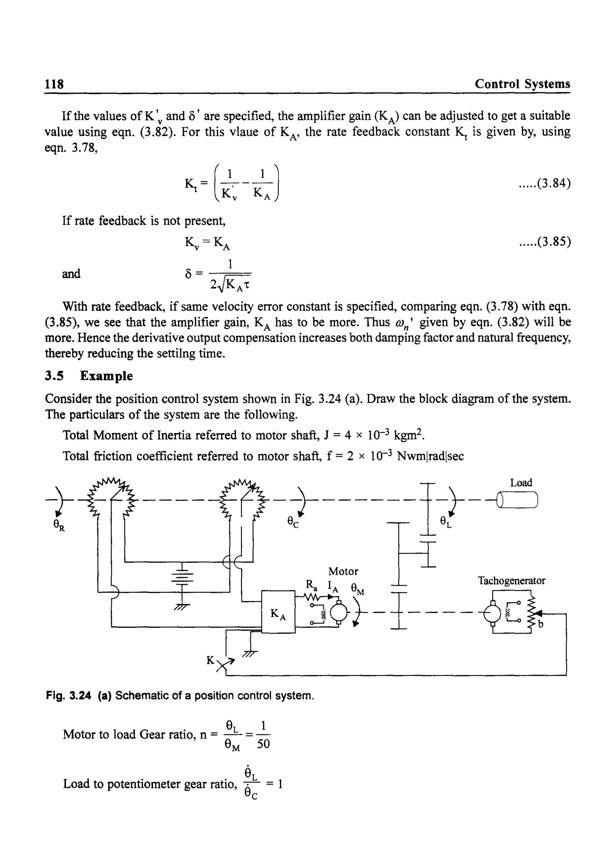
23. 14
Solution:
Writing the loop equations
(3 + s) 11(s)
- (2 + s) 11(s)
Solving for I(s), we have
- (s + 2) 12 (s)
+ (3 + 2s) 12 (s) - s.l(s)
3+s -(s + 2) yes)
- (2 +s) (3 + 2s) 0
0 -s 0
I(s) =
,
3+s -(s + 2) 0
- (2+s) (3 + 2s) -s
0 -s (1+2S+ ;s)
Yes) [s(s + 2)]
s(s + 2) V(s).2s
I(s) - ----'-:----'--:;-'--'-----;:----
- -(s+3)(4s4 + 12s3 +9s2 +4s+1)
I(s) _ 2S2(S+2)
Yes) -- (s+3)(4s4 + 12s3 t9s2 +4s+1)
2.2.2 Dual Networks
= Yes)
=0
Control Systems
.....(1)
.....(2)
.....(3)
Consider the two networks shown in Fig. 2.5 and Fig. 2.6 and eqns. (2.13) and (2.19). In eqn. (2.13)
ifthe variables q and v and circuit constant RLC are replaced by their dual quantities as per Table 2.1
eqn. (2.19) results.
Table 2.1 Dual Quantities
vet) B i(t)
i(t) B vet)
1
R B -=G
R
C B L
L B C
q = fidt B 'l' = fvdt

24. Mathematical Modelling of Physical Systems 15
The two networks, are entirely dissimilar topologically, but their equations are identical. Ifthe
solution of one equation is known, the solution of the other is also known.
Thus the two networks in Fig. 2.5 and 2.6 are known as dual networks. Given any planar
network, a dual network can always be obtained using Table 2.1.
2.2.3 Mechanical Systems
Mechanical systems can be divided into two basic systems.
(a) Translational systems and (b) Rotational systems
We will consider these two systems separately and describe these systems in terms of three
fundamental linear elements.
(a) Translational systems:
1. Mass: This represents an element which resists the motion due to inertia. According to
Newton's second law of motion, the inertia force is equal to mass times acceleration.
dv d2
x
f, =Ma=M.- =M-
M ~ ~2
.....(2.22)
Where a, v and x denote acceleration, velocity and displacement of the body respectively.
Symbolically, this element is represented by a block as shown in Fig. 2.8(a).
(a) (b) (c)
Fig. 2.8 Passive linear elements of translational motion (a) Mass (b) Dash pot (c) Spring.
2. Dash pot: This is an element which opposes motion due to friction. If the friction is viscous
friction, the frictional force is proportional to velocity. This force is also known as dampling
force. Thus we can write
dx
f =Bv=B-
B dt
.....(2.23)
Where B is the damping coefficient. This element is called as dash pot and is symbolically
represented as in Fig. 2.8(b).
3. Spring: The third element which opposes motion is the spring. The restoring force ofa spring
is proportional to the displacement. Thus
fK = K x .....(2.24)
Where K is known as the stiffness of the spring or simply spring constant. The symbol used
for this element is shown in Fig. 2.8(c).

25. 16 Control Systems
(b) Rotational systems: Corresponding to the three basic elements oftranslation systems, there are
three basic elements representing rotational systems.
1. Moment ofInertia: This element opposes the rotational motion due to Moment oflnertia. The
opposing inertia torque is given by,
dro d2
eT =Ja=J - =J-
I dt dt2 .....(2.25)
Where a, OJ and () are the angular acceleration, angular velocity and angular displacement
respectively. J is known as the moment of inertia ofthe body.
2. Friction: The damping or frictional torque which opposes the rotational motion is given by,
de
T =Bro=B-
B dt
Where B is the rotational frictional coefficient.
.....(2.26)
3. Spring: The restoring torque of a spring is proportional to the angular displacement () and is
given by,
.....(2.27)
Where K is the torsimal stiffness of the spring. The three elements defined above are shown
in Fig. 2.9.
J
Fig. 2.9 Rotational elements
Since the three elements ofrotational systems are similar in nature to those oftranslational systems
no separate symbols are necessary to represent these elements.
Having defined the basic elements ofmechanical systems, we must now be able to write differential
equations for the system when these mechanical systems are subjected to external forces. This is
done by using the D' Alembert's principle which is similar to the Kirchhoff's laws in Electrical
Networks. Also, this principle is a modified version of Newton's second law of motion. The
D' Alembert's principle states that,
"For any body, the algebraic sum ofexternally appliedforces and theforces opposing the motion
in any given direction is zero".
To apply this principle to any body, a reference direction of motion is first chosen. All forces
acting in this direction are taken positive and those against this direction are taken as negative. Let us
apply this principle to a mechanical translation system shown in Fig. 2.10.
A mass M is fixed to a wall with a spring K and the mass moves on the floor with a viscous
friction. An external force f is applied to the mass. Let us obtain the differential equation governing
the motion of the body.

26. Mathematical Modelling of Physical Systems 17
x
f
Fig. 2.10 A mechanical translational system
Let us take a reference direction of motion ofthe body from left to right. Let the displacement of
the mass be x. We assume that the mass is a rigid body, ie, every particle in the body has the same
displacement, x. Let us enumerate the forces acting on the body.
(a) external force = f
(b) resisting forces :
(i) Inertia force, fM = _ M d2~
dt
dx
(ii) Damping force, fB = - B dt
(iii) Spring force, fK = - Kx
Resisting forces are taken to be negative because they act in a direction opposite to the chosen
reference direction. Thus, using D' Alemberts principle we have,
f-M d
2
x_ B dx -Kx
dt2 dt
=0
d2
x dx
M-+B-+Kx =f
dt2 dt
or .....(2.28)
This is the differential equation governing the motion of the mechanical translation system. The
transfer function can be easily obtained by taking Laplace transform of eqn (2.28). Thus,
Xes)
--=-~---
F(s) MS2 + Bs+ K
If velocity is chosen as the output variable, we can write eqn. (2.28) as
du
M - + Bu + K Iu dt = f
dt
.....(2.29)
Similarly, the differential equation governing the motion ofrotational system can also be obtained.
For the system in Fig. 2. I 1, we have
d2
e deJ -2 + B-+Ke = T .....(2.30)
dt dt

27. 18
The transfer function of this system is given by
9(s)
--=-----
T(s) Js2
+Bs+K
Control Systems
J
Fig. 2.11 Mechanical rotatinal system
Since eqn. (2.28) and eqn. (2.30) are similar, if the solution of one system is known, the solution
for the other system can be easily obtained. Such systems are known as analogous systems. Further,
the eqns. (2.15) and (2.19) of the electrical systems shown in Fig. 2.5 and 2.6 are similar to
eqns. (2.28) and (2.30) of mechanical systems ofFigures 2.10 and 2.11. Hence the electrical systems
in Figures 2.5 and 2.6 are also analogous to mechanical systems in Figures 2.10 and 2.11.
2.2.4 Analogous Systems
Analogous systems have the same type of equations even though they have different physical
appearance. Mechanical systems, fluid systems, temperature systems etc. may be governed by the
same types ofequations as that ofelectrical circuits. In such cases we call these systems as analogous
systems. A set ofconvenient symbols are already developed in electrical engineering which permits a
complex system to be represented by a circuit diagram. The equations can be written down easily for
these circuits and the behaviour of these circuits obtained. Thus if an analogous electrical circuit is
visualised for a given mechanical system, it is easy to predict the behaviour of the system using the
well developed mathematical tools of electrical engineering. Designing and constructing a model is
easier in electrical systems. The system can be built up with cheap elements, the values of the
elements can be changed with ease and experimentation is easy with electrical circuits. Once a circuit
is designed with the required characteristics, it can be readily translated into a mechanical system. It
is not only true for mechanical systems but also several other systems like acoustical, thermal, fluid
and even economic systems.
The analogous electrical and mechanical quantities are tabulated in Table 2.2.
Table 2.2 Analogous quantities based on force voltage analogy
Electrical system Mechanical system
Translational Rotational
Voltage V Force f Torque T
Current i Velocity u angular velocity (j)
Charge q Displacement x angular displacement 9
Inductance L Mass M Moment ofInertia J
1 1
Capacitance C Compliance - Compliance -
K K
Resistance R Damping coefficient B Damping coefficient B

28. Mathematical Modelling of Physical Systems 19
Comparing the eqn. (2.15) ofthe electrical system and eqn. (2.28) and eqn. (2.30) ofmechanical
systems it is easy to see the correspondence ofthe various quantities in Table 2.2. Since the external
force applied to mechanical system, fl' is made analogous to the voltage applied to the electrical
circuit, this is called as Force - Voltage analogy.
If the mechanical systems are compared with the electrical circuit in Fig. 2.6, in which the
source is a current source, force applied in mechanical system is analogous to the current. The
analogous quantities based on force-current analogy are given in Table 2.3
The Table 2.3 can be easily understood by comparing eqn. (2.19) ofthe electrical system with
eqns. (2.28) and (2.30) of mechanical systems.
Table 2.3 Analogous quantities based on Force - Current analogy
Electrical system Mechanical system
Translational Rotational
Current i Force f Torque T
Voltage v Velocity u angular velocity (0
Flux linkages 'I' Displacement x angular displacement e
Capacitance C Mass M Moment ofInertia J
Conductance G Damping coefficient B Rotational Damping coefficient B
I 1
Inductance L Compliance - Compliance -
K K
Now let us consider some examples of mechanical systems and construct their
mathematical models.
Example 2.4
Write the equations describing the motion of the mechanical system shown in Fig. 2.12.
Also find the transfer function Xj(s)lF(s).
Fig. 2.12 A Mechanical system for example 2.4
Solution:
The first step is to identify the displacements of masses Mj and M2 as Xj and x2in the direction ofthe
applied external force! Next we write the equilibrium equation for each ofthe masses by identifying
the forces acting on them. Let us first find out the forces acting on mass M j •

29. 20
External force = f
Restoring forces :
d2
x
(i) Inertia forc.e, - Ml -2-1
dt
(
..) . fi d
2
(XI -X2)
11 Dampmg orce, - Bl 2
dt
(iii) Spring force, - Kl (xl - x2)
(If xl > x2 the spring expands and restoring force is upwards)
Control Systems
(Note: Since top end ofdash pot and spring are rigidly connected to mass M2, their displacement
is x2 in the downward direction. Similarly, the bottom ends of dash pot spring are rigidly
connected the mass Ml' they move downward by Xl' The relative displacement of the lower
end_upper end is (xl
-x2
) in the downward direction. Hence restoring forces are-Bl d (XI - x2)
dt
and - Kl (xl - x2) respectively due to the dash pot and spring).
Hence the equation ofmotion is
Now for mass M2
External force = Zero
Restoring forces :
d2
x
(i) Inertia force, - M2 -2_2
dt
.....(1)
(li) Damping forces,
dX2
(a) - B2 dt (since one end is fixed and the other is connected to Ml rigidly)
(b) - B • d(x2 - XI) (If dx2 > dXI , the motion is in the downward direction and
1 dt dt dt
(iii) Spring forces :
(a) - K2 x2
the frictional force is in the upward direction)
(b) - Kl (Xz - Xl) (If Xz > Xl' the spring is compressed and the restoring force
is upward)

30. Mathematical Modelling of Physical Systems 21
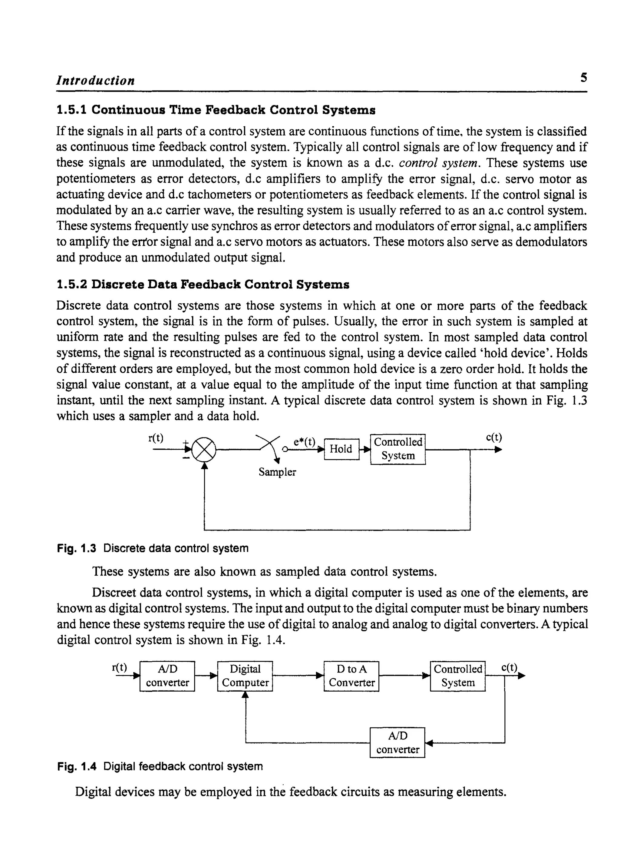
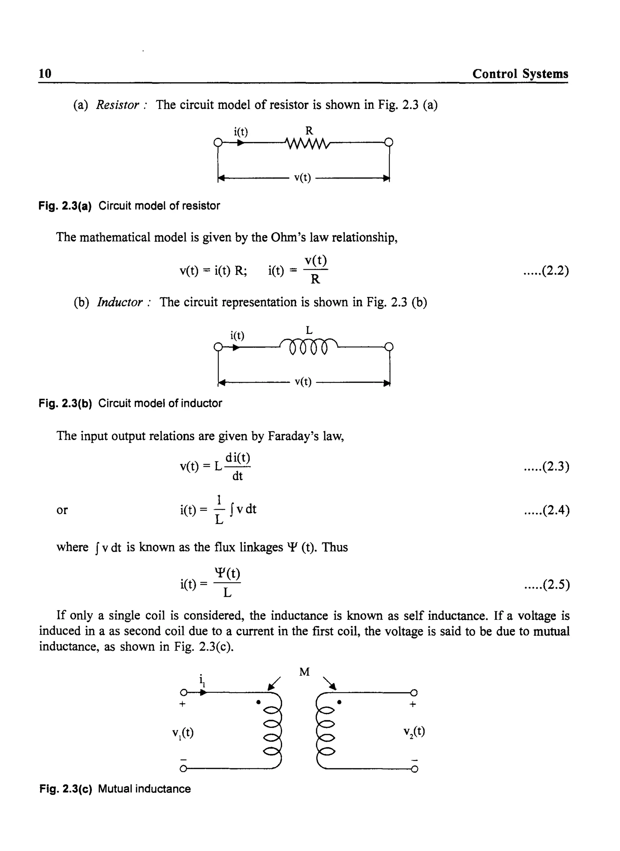
Hence the equation of motion for M2 is,
d
2
x2 dX2 d(x2 - Xl)
M2 ~+B2~+BI dt +K2X2+KI(X2-XI) =0 ....(2)
From eqns. (l) & (2), force voltage analogous electrical circuits can be drawn as shown in Fig. 2.13 (a).
v[t]
Fig. 2.13 (a) Force - Voltage analogous circuit for mechanical system of Fig. 2.12. Mechanical quantities
are shown in parenthesis
Force - current analogous circuit can also be developed for the given mechanical system. It is
given in Fig. 2.13 (b). Note that since the mass is represented by a capacitance and voltage is
analogous to velocity, one end ofthe capacitor must always be grounded so that its velocity is always
referred with respect to the earth.
XI(s)
= - -
F(s)
Transfer function
Taking Laplace transform of eqns. (1) and (2) and assuming zero initial conditions, we have
MI s2 XI (s) + BI s [XI (s) - X2 (s)] + KI [XI(s) - X2 (s)] = F(s)
or (MI s2 + Bls + KI) XI (s) - (BI S + KI) X2 (s) = F(s) .....(3)
and M2 s2 X2 (s) + B2 s X2(s) + BI s [Xis) - XI(s)] + K2 X2 (s)
+ KI [(~ (s) - XI(s)] = 0
or - (Bls + KI) XI(s) + [M2s2 + (B2 + BI)s + (K2 + KI) Xis) = 0 .....(4)
Fig. 2.13 (b) Force current analogous circuit for the mechanical system of Fig. 2.12

31. 22 Control Systems
Solving for Xis) in eqn (4), we get
Bjs+Kj X ()
Xis) = M2 S2 +(Bj + B2)s+(Kj + K2) j s
Substituting for Xis) in eqn. (3)
(M/+Bjs+Kj)Xj(s)- (~jS+Kj).(BjS+Kj) Xj(s) =F(s)
M2s +(Bj +B2)s+Kj +K2
Xj(s) = M2s2 +(Bj +B2)S+Kj +K2 F(s)
MjS2 + Bj s+Kj M2 S2 +(Bj + B2)s+(Kj + K2) -(Bj S+Kj)2
Thus
Xj(s) M2s2 +(Bj +B2}s+Kj +K2
T(s) = F(s) = (Mj s2
+BjS+Kj)[M2
s2 +(Bj +B2)S+(Kj +K2
)J-(Bjs+Kj)2
Which is the desired transfer function.
Example 2.5
Obtain the f-v and f-i analogous circuits for the mechanical system shown in Fig. 2.14. Also
write down the equilibrium equations.
Fig. 2.14 Mechanical system for Ex. 2.5
Solution:
Let f be the force acting on the spring instead of velocity u. The displacements are indicated in the
figure.
The equilibrium equations are:
K (Xj -~) = f
B ("2 - '(3) + K (X2- Xj) = 0
B ("3 - '(2) + M X3= 0
From eqs (1) and (2), we have
B ("2 - '(3) = f
From eqs (3) and (4), we have
MX3 =f
.....(1)
.....(2)
.....(3)
.....(4)
.....(5)

32. Mathematical Modelling of Physical Systems 23
Force CurrentAnalogous Circuit
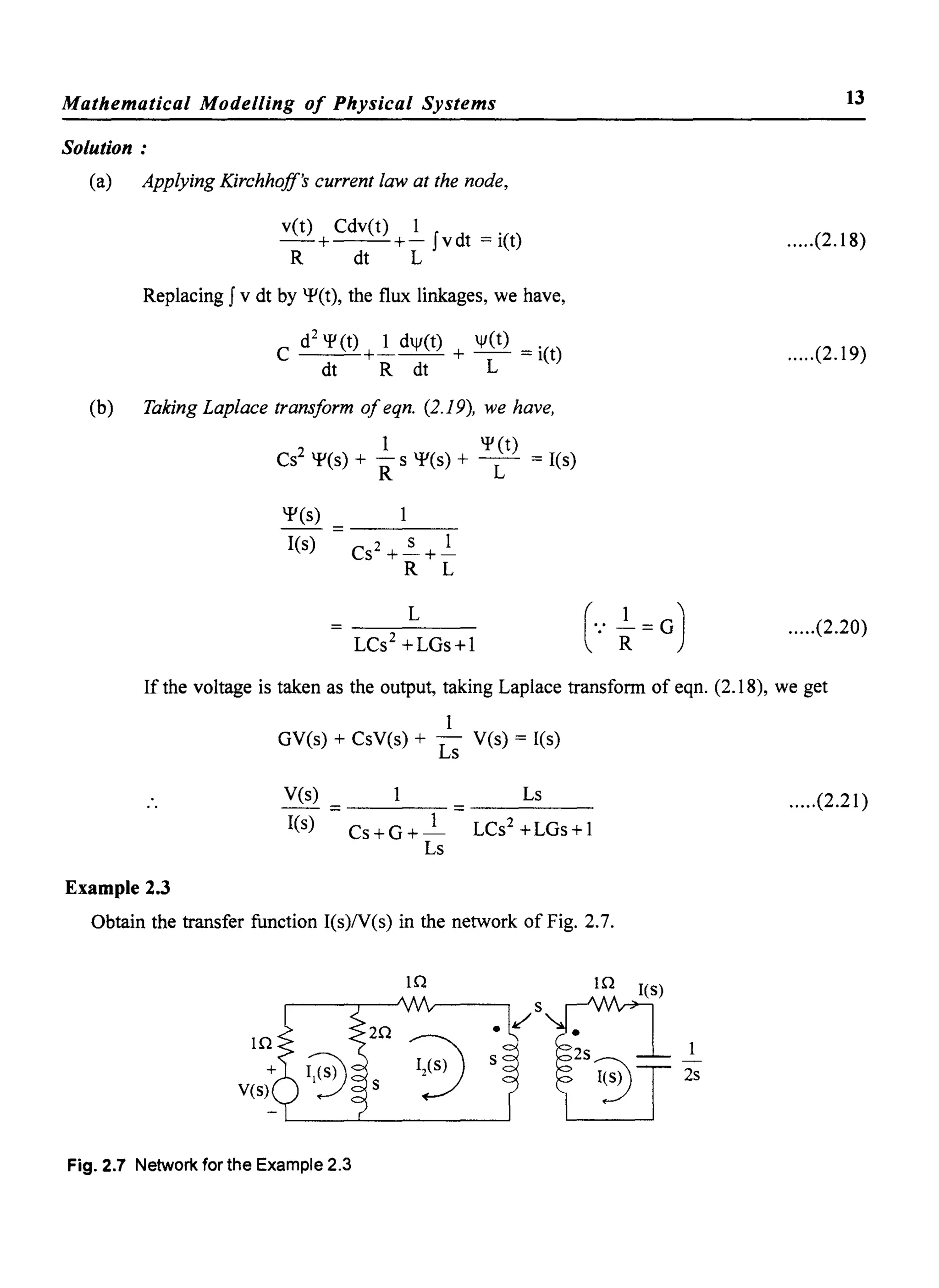
Replacing the electrical quantities in equations (1), (4), and (5) by their force-current analogous
quantities using Table 2.3, we have
or
or
or
~f (v - v )dt = i
L ' 2
G (q,2 - q,3) = i
G(V2 - V3) = i
..
C 'f'3 = i
C dV3 = i
dt
.....(6)
.....(7)
.....(8)
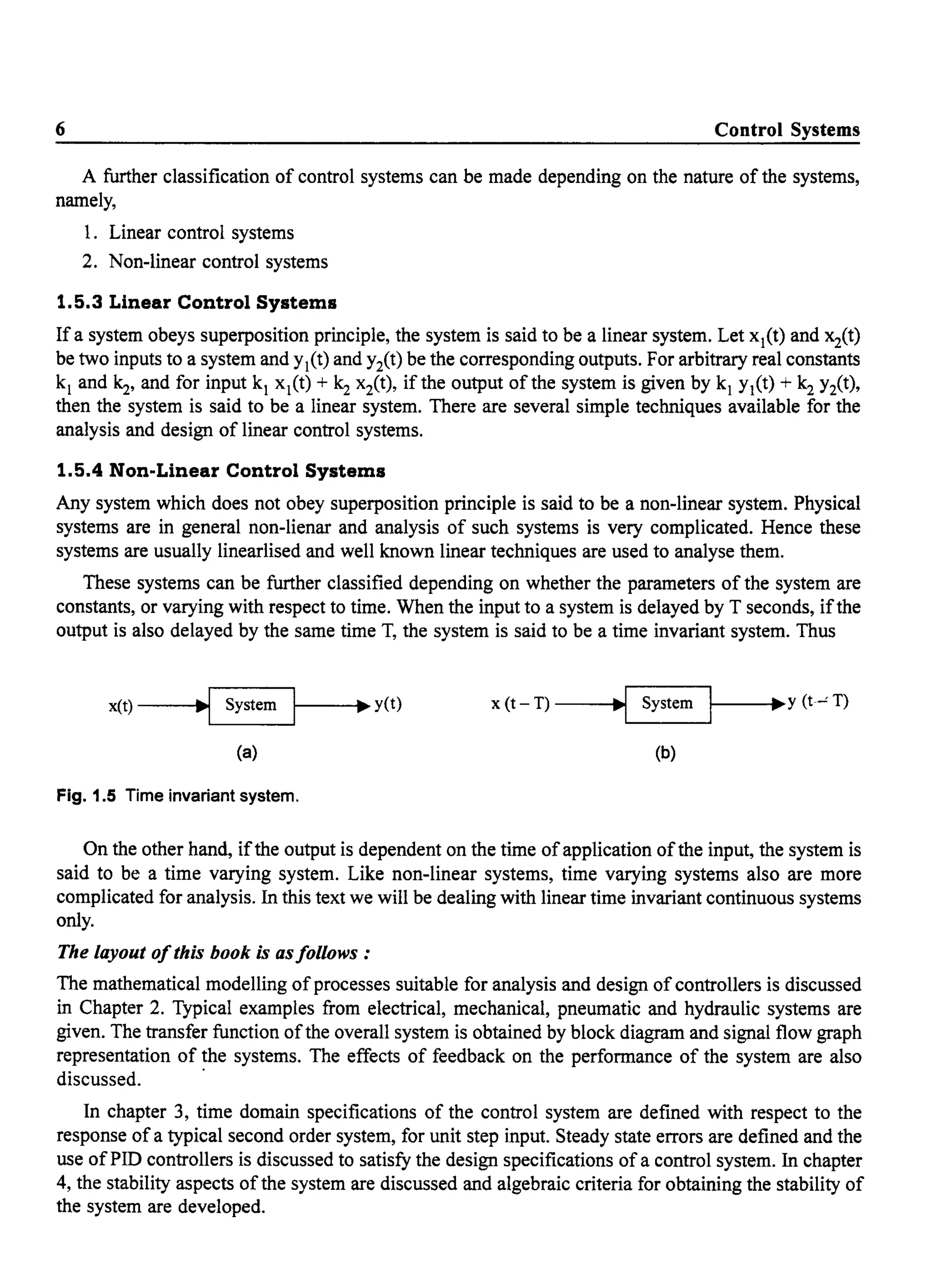
If i is produced by a voltage source v, we have the electrical circuit based on f-i analogy in
Fig. 2.14 (a).
G[B]
v[u]
C[M]
Fig. 2.14 (a) F-i analogous circuit for mechanical system in Ex. 2.5
Force Voltage Analogous Circuit
Using force voltage analogy, the quantities in eqs (1), (4) and (5) are replaced by the mechanical
quantities to get,
or
or
1
-(q -q ) = v
C ' 2
~f(i, - i2) dt = v
C
R «h -qJ = v
R (i2 - i3) = v
d
2
q3
L--=v
dt2
.....(9)
.....(10)

33. 24 Control Systems
or
di3
L-=v
dt
.....(11)
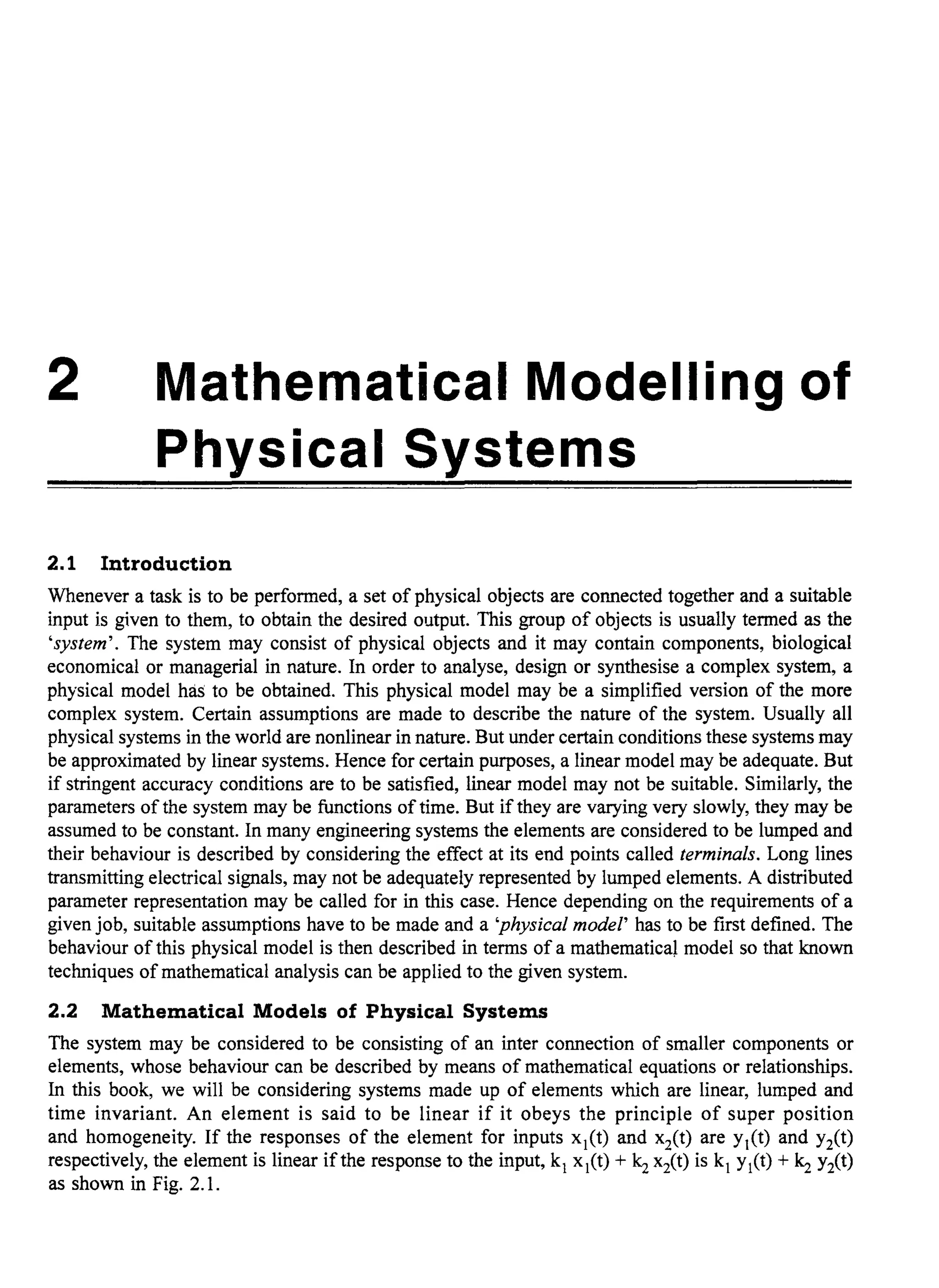
If the voltage is due to a current source i, we have the force voltage analogous circuit is shown in
Fig. 2.14 (b)
+
v[f]
R[B] L[M]
Fig. 2.14 (b) Force voltage analogous circuit for the mechanical system of Ex. 2.5
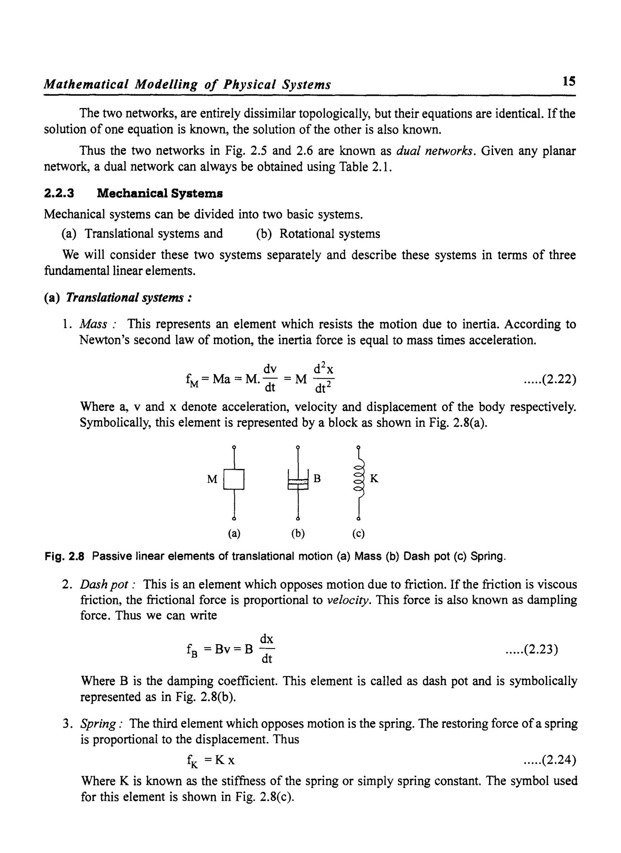
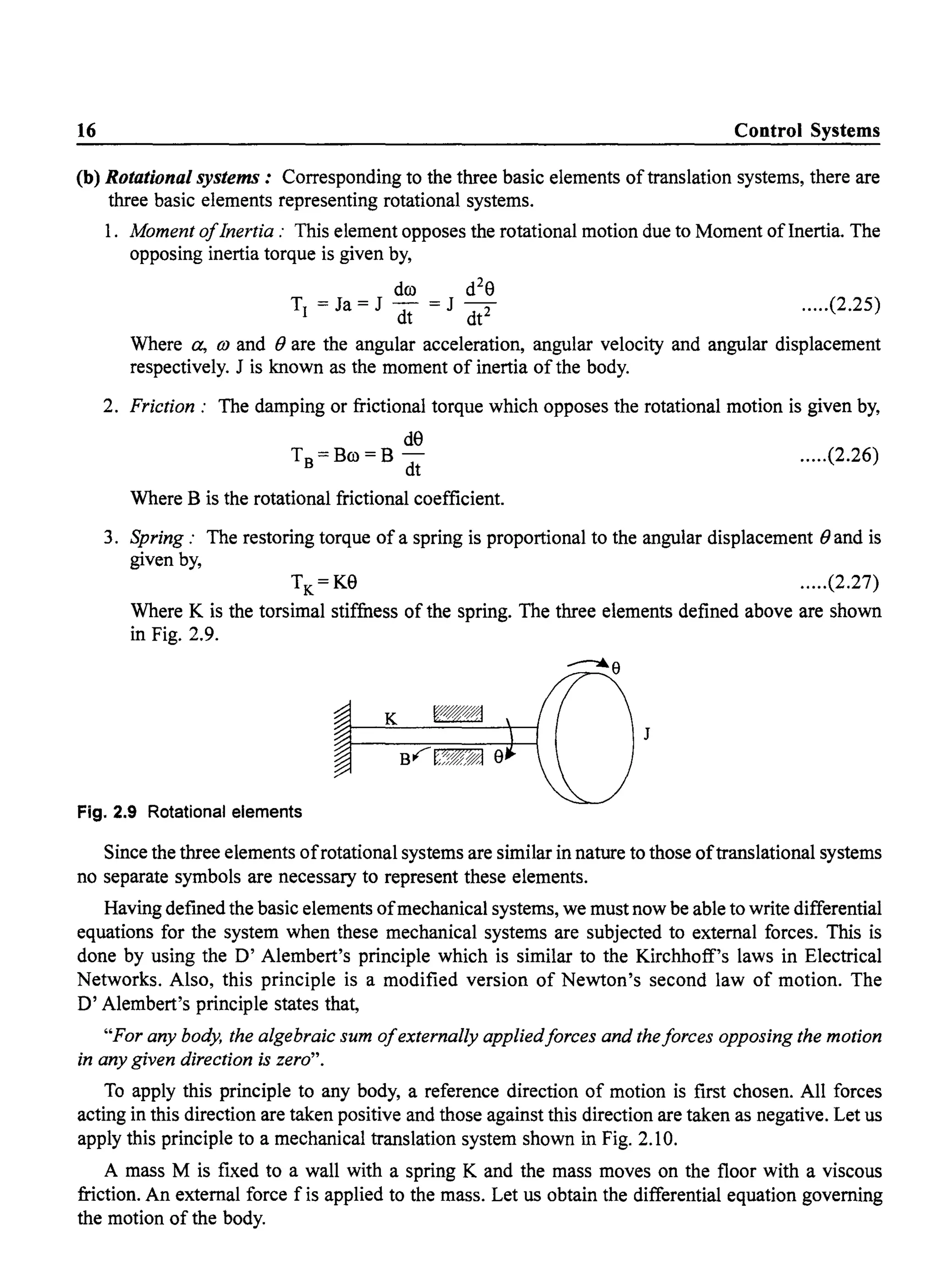
2.2.5 Gears
Gears are mechanical coupling devices used for speed reduction or magnification of torque. These
are analogous to transformers in Electrical systems. Consider two gears shown in Fig. 2.15. The first
gear, to which torque T1 is applied, is known as the primary gear and has N1 teeth on it. The second
gear, which is coupled to this gear and is driving a load, is known as the secondary gear and has N2
teeth on it.
Fig. 2.15 Geartrain
The relationships between primary and secondary quantities are bas~d on the following principles.
1. The number of teeth on the gear is proportional to the radius of the gear
r N
-=-
2. The linear distance traversed along the surface of each gear is same.
If the angular displacements of the two gears are ()1 and 82 respectively, then
r1 91 =r2 92
!.L=~
r2 9
.....(2.31)
.....(2.32)

34. Mathematical Modelling of Physical Systems
3. The work done by one gear is same as that of the other.
If T1 and T2 are the torques on the two gears,
TI 01 = T2 02
Using eqs (2.31), (2.32) and (2.33), we have,
°1 T2 N2-=-=-
Recall that, for an ideal transformer of primary tums N1 and secondary turns N2,
VI 12 NI
-=-=
V2 II N2
25
.....(2.33)
.....(2.34)
.....(2.35)
Eqn. (2.35) is similar to eqn. (2.34) and hence a gear train in mechanical system is analogous
to an ideal transformer in the electrical system.
Writing the equilibrium equations for the mechanical system of Fig. (2.14), we have
.....(2.36)
.....(2.37)
Where TM is the motor torque driving the shaft of the gear, T1 is the torque available for the
primary gear, T2 is the torque at the secondary gear, TL is the load torque and J2 is the moment
of inertia of secondary gear and the load.
Using eqn. (2.34) in eqn. (2.37), we have
.....(2.38)
Substituting for TI in eqn. (2.36), using eqn. (2.38),
But,
and
JI '91 + BI 91 + KI °1 + ~. (J2 '0'2 + B2 92 + K2 O2 + T L) = TM .....(2.39)
N2
°=~O2 N I
2

35. 26 Control Systems
Using these relations in eqn. (2.39), we get
.....(2.40)
Replacing
and
We have,
JI eq ·e· + BI 9 + K leq el + T Leq = TM .....(2.41)
Thus the original system in Fig. 2.15 can be replaced by an equivalent system referred to
primary side as shown in Fig. 2.16.
Fig. 2.16 Equivalent system refered to primary side
.The moment of inertia J2, frictional coefficient B2 and torsional spring constant K2 of secondary
side are represented by their equivalents referred to primary side by,
J12 ~J, (~:r
B12~B,(~:r

36. Mathematical Modelling of Physical Systems
The load torque referred to primary side is given by,
_ Nl
TLeq-TL · -
N2
27
These equations can be easily seen to be similar to the corresponding electrical quantities in the
ideal transformer.
All the quantities can also be referred to the secondary side ofthe gear. The relevant equations are
.lzeq ·9~ + B2eq 92 + K2eq 92 + TL = TMeq .....(2.42)
where J2,q~J2+JI (::rB2,,~B2+BI (::J
and
2.2.6 Thermal Systems
Thermal systems are those systems in which heat transfer takes place from one substance to another.
They can be characterised by thermal resistance and capacitance, analogous to electrical resistance
and capacitance. Thermal system is usually a non linear system and since the temperature of a
substance is not uniform throughout the body, it is a distributed system. But for simplicity ofanalysis,
the system is assumed to be linear and is represented by lumped parameters.
(a) Thermal resistance
There are two types of heat flow through conductors : Conduction or convection and radiation.
Fig. 2.17 Thermal resistance
For conduction of heat flow through a specific conductor, according to Fourier law,
......(2.42)

37. 28
where,
q = Heat flow, Joules/Sec
K = Thermal conductivity, J/sec/m/deg k
A = Area normal to heat flow, m2
~X = Thickness of conductor, m
8 = Temperature in oK
For convection heat transfer,
q = HA (81 - 82)
where H = Convection coefficient, J/m~/sec/deg k
The thermal resistance is defined by,
d8 ~X
R = - = -
dq KA
(Conduction)
HA
(Convection)
The unit of R is deg seclJ
Control Systems
.....(2.43)
.....(2.44)
.....(2.45)
For radiation heat transfer, the heat flow is governed by Stefan-Boltzmann law for a surface
receiving heat radiation from a black body:
q = KAE (84
1 - 84
2)
= A cr (8 - 84
2) .....(2.46)
where,
cr is a constant, 5.6697 x 10-8
J/sec/m2
/K4
K is a constant
E is emissivity
A is surface in m2
The radiation resistance is given by
d8 1
R = -d = 3 deg sec/J .....(2.47)
q 4Acr8a
where 8a is the average temperature ofradiator and receiver. Since eqn. (2.46) is highly nonlinear,
it can be used only for small range of temperatures.
(b) Thermal Capacitance
Thermal capacitance is the ability to store thermal energy. If heat is supplied to a body, its internal
energy raises. For the system shown in Fig. 2.18,
Fig. 2.18 Thermal CapaCitance

38. Mathematical Modelling of Physical Systems
where
where
de
C- =q
dt
C is the thennal capacitance
C=WCp
W ~ weight of block in kg
Cp ~ specific heat at constant pressure in J/deg/kg
2.2.7' Fluid Systems
29
.....(2.48)
.....(2.49)
Fluid systems are those systems in which liquid or gas filled tanks are connected through pipes,
tubes, orifices, valves and other flow restricting devices. Compressibility of a fluid is an important
property which influences the perfonnance of fluid systems. Ifthe velocity ofsound in fluids is very
high, compared to the fluid velocity, the compressibility can be disregarded. Hence compressibility
effects are neglected in liquid systems. However compressibility plays an important role in gas systems.
The type offluid flow, laminar or turbulent, is another important parameter in fluid systems. Ifthe
Reynolds number is greater than 4000, the flow is said to be turbulent and ifthe Reynolds number is
less than 2000, it is said to be laminar flow.
For turbulent flow through pipes, orifices, valves and other flow restricting devices, the flow is
found from Bernoulli's law and is given by
q =KA ~2g(hl -h2) .....(2.50)
where q ~ liquid flow rate, m3
/sec
K ~ a flow constant
A ~ area of restriction, m2
g is acceleration due to gravity, mlsec2
h head of liquid, m
The turbulent resistance is found from
.....(2.51)
It can be seen that the flow resistance depends on hand q and therefore it is non linear. It has to
be linearised around the operating point and used over a small range around this point.
The laminar flow resistance is found from the Poisseuille - Hagen law "
128j..lL
hi - h2 = nyD4 q .....(2.52)
where h ~ head, m
L ~ length of the tube, m
D ~ inside diameter of the pipe, m

39. 30
q ~ liquid flow rate, m3/sec
m ~ absolute viscosity, kg-sec/m2
y ~ fluid density kg/m3
Control Systems
Since the flow is laminar, head is directly proportional to the flow rate and hence, laminar flow
resistance is given by
R = 128 ~ sec/m2
1tYD4
Liquid storage tanks are characterised by the capacitance and is defined by,
dv
C=- m2
dh
.....(2.53)
.....(2.54)
where v ~ volume of the liquid tank in m3
. Hence the capacitance ofa tank is given by its area
of cross section at a given liquid surface.
Gas systems consisting of pressure vessels, connecting pipes, valves etc. may be analysed by
using the fundamental law of flow of compressible gases. Again, we have to consider two types of
flow: turbulent and laminar flow. For turbulent flow through pipes, orifices, valves etc., we have
where
0)=KAY~2g (pl -P2)Y
0) ~ flow rate, kg/sec
K ~ flow constant
A ~ area of restriction, m2
y ~ gas density, kg/m3
p ~ pressure in kg/m2
Turbulent gas flow resistance is therefore given by
R= ~ sec/m2
dw
.....(2.55)
.....(2.56)
This is not easy to determine since the rational expansion factor depends on pressure. Usually the
resistance is determined from a plot of pressure against flow rate for a given device.
The laminar gas flow resistance is obtained using eqn. (2.50).
P_l~______~I~rl________P~2
resistance R
Fig. 2.19 Gas resistance and capacitance
The capacitance parameter for pressure vessels is defined as
dv
C =--
dp
Capacitance C
.....(2.57)

40. Mathematical Modelling 0/ Physical Systems
where v -+ weight of gas in vessel, kg
p -+ pressure kg/m2
The flow rate and the gas pressure are related by the continuity law :
dp
C- =0)
dt
Where OJ is the flow rate in kg/sec.
31
.....(2.58)
Let us now consider some thennal and fluid systems and obtain their transfer functions.
Example 2.6
Find the transfer function C(s) of the thennal system shown in Fig. 2.20. Heat is supplied by
yes)
convection to a copper rod of diameter O.
Fig. 2.20 Thermal System
Solution:
u (temperature)
-..Convection
Copper rod
C (temperature)
4+--
The Thennal resistance of the copper rod, from eqn. (2.45), is;
I
R=-
HA
Here A is the surface area of the rod.
Hence A = 7t OL
where L is the length of the rod.
I
.. R = 7t OL deg sec/J
The thennal capacitance of the rod, from eqn. (2.49), is given by :
C=WCp
7t02
L
= -4- pCp
where, Cp is the specific heat of copper
and p is the density of copper.
From eqn. (2.43), we have, q = HA (u - c) and from eqn. (2.48),
dc
C - =q
dt
Combining these two equations,
dc I
C -=- (u-c)
dt R

41. 32
C dc +~=~
dt R R
dc
RC - +c=u
dt
where RC = T is the time constant of the system.
dc
T-+c=u
dt
1 1t02
L
T=RC= --x--pCp
1tDLH 4
But
= DpCp
4H
Thus the transfer function of the system is,
C(s)
- - = - - where
U(s) Ts+l
DpCp
T=--
4H
Control Systems
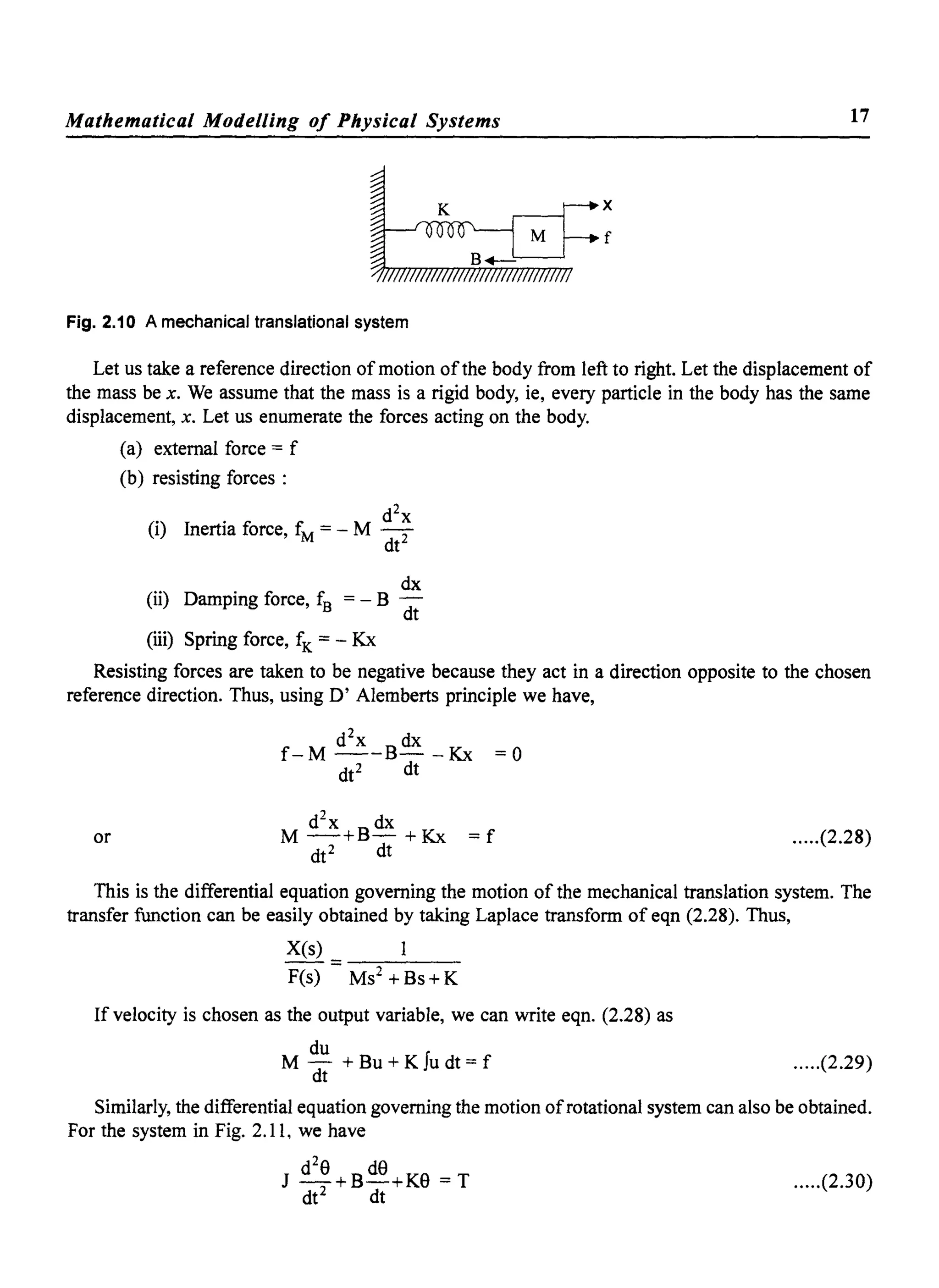
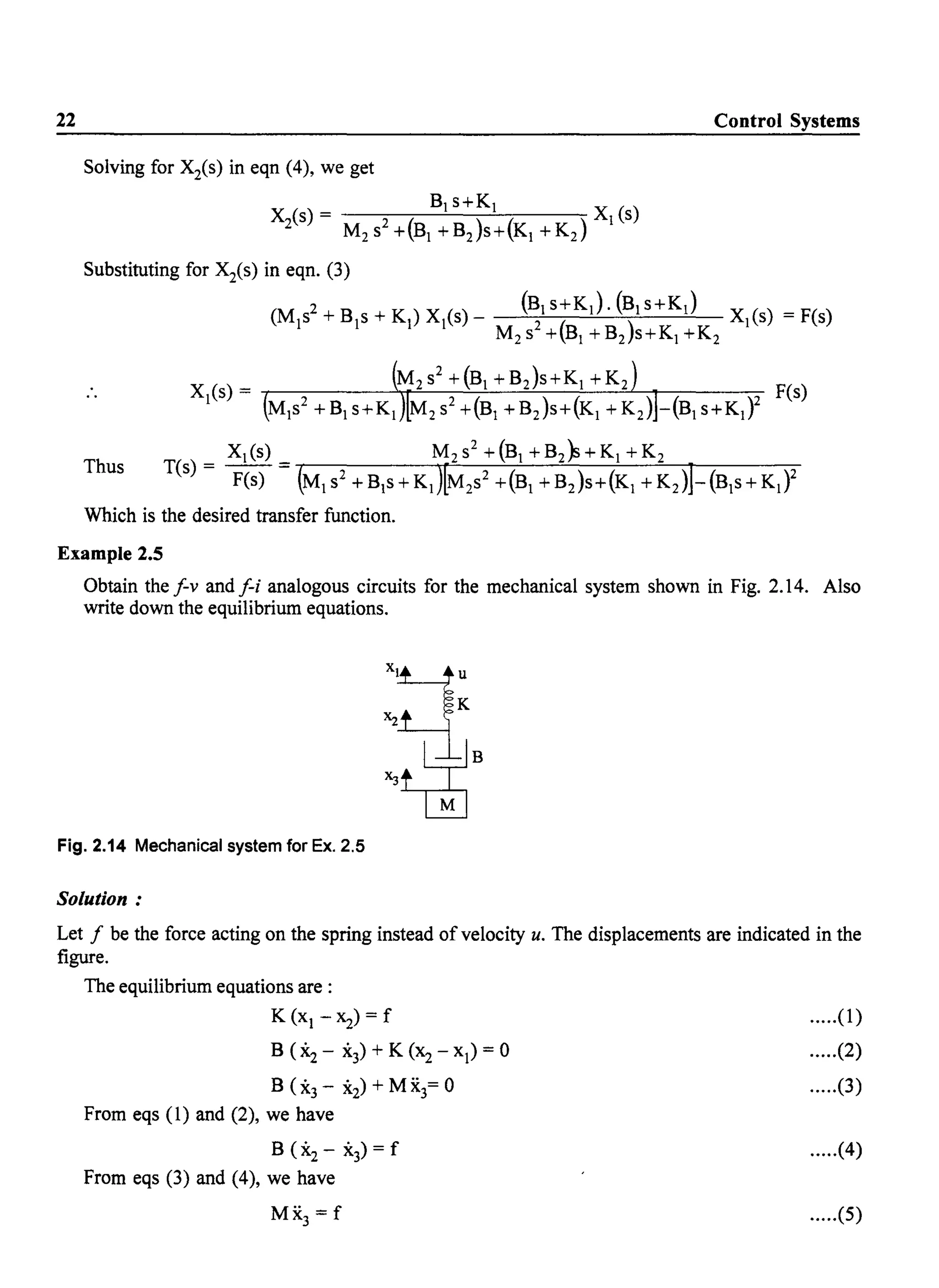
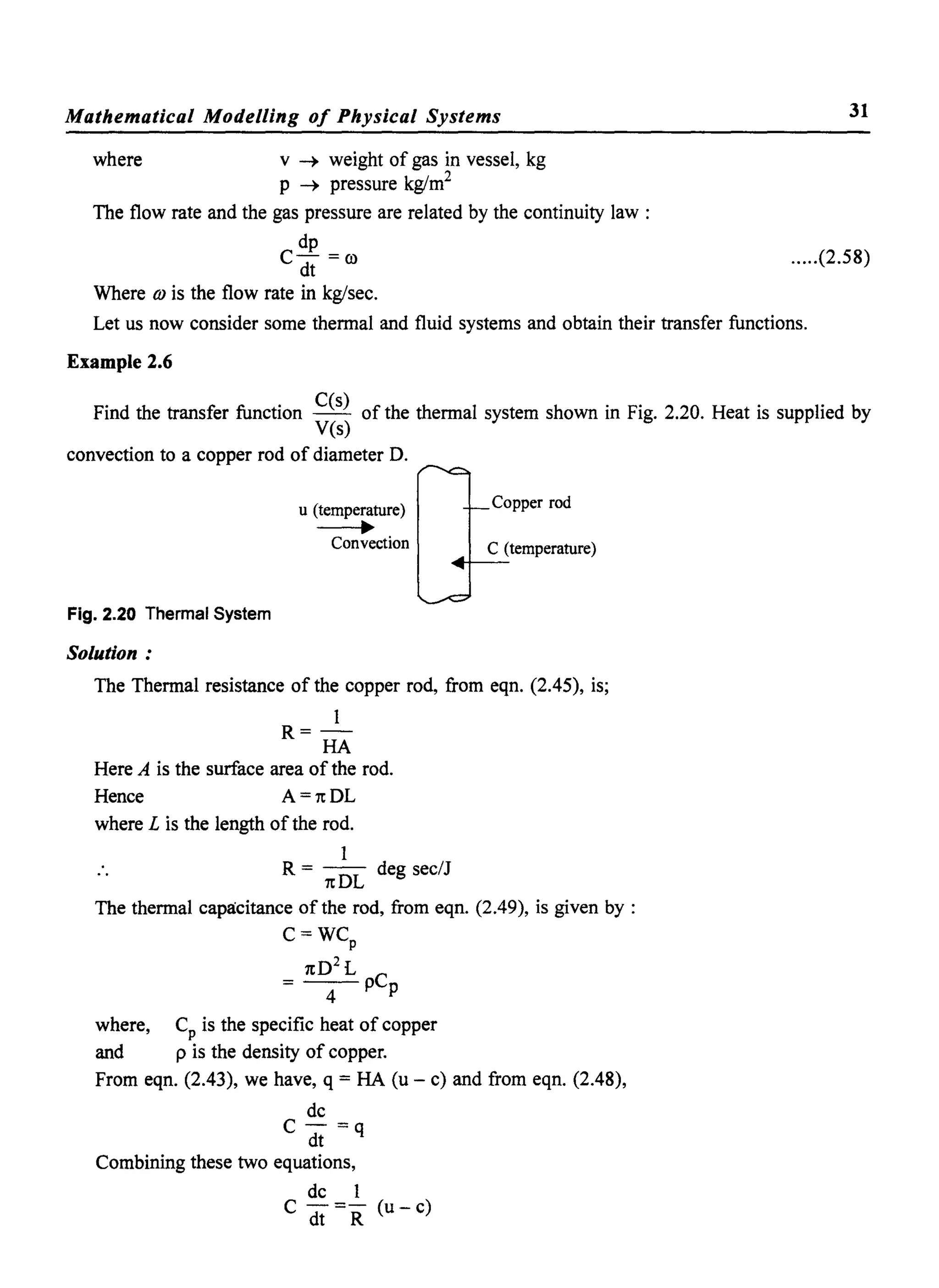
Example 2.7
Obtain the transfer function C(s) for the system shown in Fig. 2.21. c is the displacement of the
U(s)
piston with mass M.
u, pressure ~
B,damping f- M, mass
Gas ~:Area
Fig. 2.21 A fluid system
Solution: The system is a combination of mechanical system with mass M, damping B and a gas
system subjected to pressure.
The equilibrium equation is
Me +Bc=A[U-Pg] .....(2.1)
Where Pg is the upward pressure exerted by the compressed gas. For a small change in displacement
of mass, the pressure exerted is equal to,
P
P = - Ac
g V
where, P is the pressure exerted by the gas with a volume of gas under the piston to be V
But PV= WRT
where, R is the gas constant.

42. Mathematical Modelling of Physical Systems
and T is the temperature of the gas.
WRT
p = ---v-
WRT
P = --Ac
g y2
Substituting eqn. (2) in eqn. (1) we have,
WRT
Me + B c + --2- A2c = A u
Y
The transfer function is,
C(s) A
U(s) MS2 +Bs+K
WRT 2
where K = - - P:.
y2
Example 2.8
Obtain the transfer function for the liquid level system shown in Fig. 2.22.
c
Fig. 2.22 Liquid level system
Solution: The capacitance of the vessel is C = A
where A is the area of cross section of the vessel.
The outflow q is equal to,
c
q= -
R
where R is the laminar flow resistance of the valve.
c
A c = (u - q) = u - -
R
c
Ac + - = u
R
The transfer function is
C(s) R
--=---
u(s) RAs+l
R
33
......(2)

43. 34 Control Systems
2.3 Block Diagrams of Closed Loop Systems
The transfer function of any system can be represented by a block diagram as shown in Fig. 2.23.
u(s) Iinput------l.~ G(s)
Fig. 2.23 Block diagram of a system
f-----I.~- C(s)
output
A complex system can be modelled as interconnection ofnumber ofsuch blocks. Inputs to certain
blocks may be derived by summing or substracting two or more signals. The sum or difference of
signals is indicated in the diagram by a symbol called summer, as shown in Fig. 2.24 (a).
+
±
(a) (b)
Fig. 2.24 (a) Symbol of a summer (b) Pick off point
On the other hand, a signal may be taken from the output of a block and given to another block.
This point from which the signal is tapped is known as pick off point and is shown in Fig. 2.24 (b).
A simple feedback system with the associated nomenclature of signals is shown in Fig. 2.25.
R(s)
+ Summer
E(s)
± pick off point
B(s)
Fig. 2.25 Simple feedback system
C(s)
G(s) = E(s); Forward path transfer function, or plant transfer function
B(s)
R(s) = E(s); Transfer function of the feedback elements
where, R(s); Reference input or desired output
C(s); Output or controlled variable
B(s); Feedback signal
E(s); Error signal
G(s) R(s); Loop transfer function
This closed loop system can be replaced by a single block by finding the transfer function ~~:~.

44. Mathematical Modelling of Physical Systems
But
C(s) = G(s) E(s)
E(s) = R(s) ± B(s)
= R(s) ± R(s) C(s)
C(s) = G(s) [R(s) ±R(s) C(s)]
C(s) [1 =+= G(s) R(s)] = G(s) R(s)
C(s) G(s)
- - = --'--'--
R(s) 1+ G(s) R(s)
This transfer function can be represented by the single block shown in Fig. 2.26.
R(s) --------1..
ao1
I1+G~;:~(S)Ir------...-C(s)
Fig. 2.26 Transfer function of the closed loop system
35
.....(2.59)
.....(2.60)
.....(2.61)
.....(2.62)
.....(2.63)
(Note : If the feedback signal is added to the reference input the feedback is said to be positive
feedback. On the other hand ifthe feedback signal is subtracted from the reference input, the feedback
is said to be negative feedback).
For the most common case of negative feedback,
C(s)
R(s)
G(s)
1+ G(s) R(s)
.....(2.64)
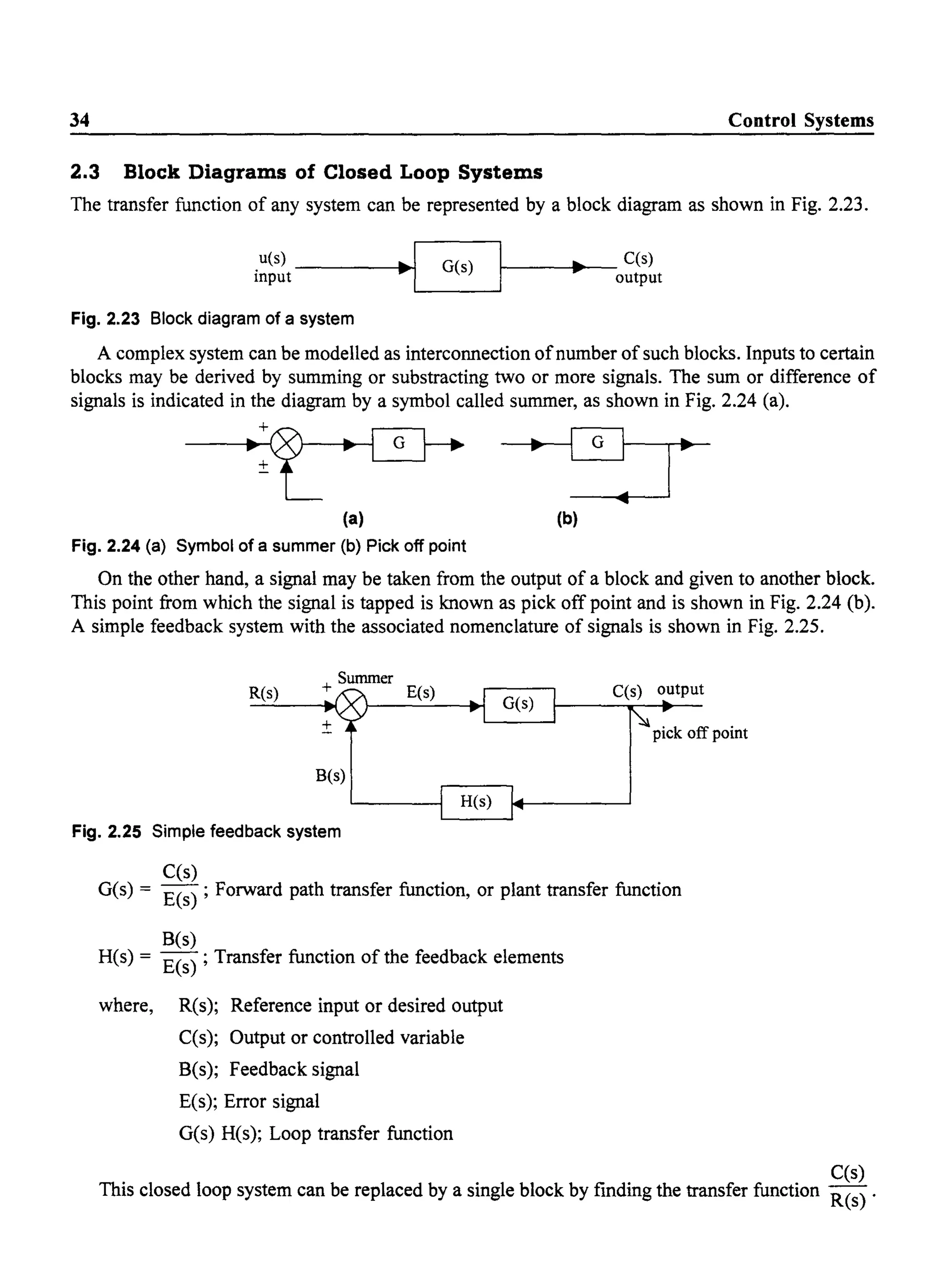
The block diagram of a complex system can be constructed by finding the transfer functions of
simple subsystems. The overall transfer function can be found by reducing the block diagram, using
block diagram reduction techniques, discussed in the next section.
2.3.1 Block Diagram Reduction Techniques
A block diagram with several summers and pick off points can be reduced to a single block, by using
block diagram algebra, consisting of the following rules.
Rule 1 : Two blocks G1 and G2 in cascade can be replaced by a single block as shown in Fig. 2.27.
Fig. 2.27 Cascade of two blocks
Rere
z
- =G
x I'
r =G
z 2
z y y
-.- = - =G G
x z X I 2
• y

45. 36 Control Systems
Rule 2 : A summing point can be moved from right side ofthe block to left side ofthe block as shown
in Fig. 2.28.
X-----1~ I----.-y = X~y
w--u}lW - - - - - - - I
Fig. 2.28 Moving a summing point to left of the block
For the two systems to be equivalent the input and output of the system should be the same. For
the left hand side system, we have,
y = G [x] + W
For the system on right side also,
y = G [x + ~ [W]] = G [x] + w
Rule 3: A summing point can be moved from left side of the block to right side of the block as
shown in Fig. 2.29.
+
x---.t
+
y=G(x+w)
=G[x]+G[w]
y
Fig. 2.29 Moving a summer to the right side of the block
x
Y = G[x] + G[w]
Rule 4: A Pick off point can be moved from the right side of the block to left side of the block as
shown in Fig. 2.30.
x
~~
~y
w
y = G[x]
w=y
y= G[x]
w =G[x] =y
Fig. 2.30 Moving a pick off point to left side of the block
Rule 5: A Pick off point can be moved from left side of the block to the right side of the block as
shown in Fig. 2.3 1.
x-'~~I-~Y
w ........I------1-
x~...----1QJ tiJ
w ........I-------'
y= G[x] y=G[x]
w=x w= i[Y]=x
Fig. 2.31 Moving a pick off point to the right side of the block

46. Mathematical Modelling of Physical Systems 37
Rule 6: A feedback loop can be replaced by a single block as shown in Fig 2.32.
x
~x - - Y
l+GH
Fig. 2.32 Feedback loop is replaced by a single block
Using these six rules. which are summerised in Table 2.4, any complex block diagram can be
simplified to a single block with an input and output. The summing points and pick off points are
moved to the left or right of the blocks so that we have either two blocks in cascade, which can be
combined, or a simple feedback loop results, which can be replaced by a single block.
This is illustrated in the following examples.
Table 2.4 Rules of Block diagram algebra
Rule no. Given system Equivalent system
1. Blocks in cascade x-1 G 1
H G2 ~Y X .. 1G1 G2 1 .. Y
2. Moving summing point to left
x-1 I
+
w~
G .yy G Y
w
X~'3. Moving summing point to right
x::f ·1
G ~Y
w G
x-1 G
I
~ y
:iJ4rl G ~y'
w:J4. Moving pick off point to left
wG
x
w;J I G
~Y X~'5. Moving pick off point to right
w J..G
6. Absorbing a loop
xL: [.: x-1 I+:H ~Y

47. 38 Control Systems
Example 2.9
Find the overall transfer function of the system shown in Fig. 2.33 using block diagram reduction
technique.
+
R(s)--.....-t ~---r--l"" C(s)
Fig. 2.33 Block diagram of a system
Solution:
Step I : Using rule 6, the feedback loop with G2 and H2 is replaced by a single block as shown
in Fig. 2.33 (a).
R(s) -----1~
B(s)
Fig. 2.33 (a)
G
2-----=-- I-----.--~~C(s)
l+G H
2 2
Step 2: The two blocks in the forward path are in cascade and can be replaced using rule I as
shown in Fig. 2.33 (b).
+
R(s)---~
Fig. 2.33 (b)
Step 3: Finally, the loop in Fig. 2.33 (b) is replaced by a single block using rule 6.
G
1
G
2
R(s) .. 1+ G
2
H2
..~
G1 G2 H1
~
1+
1---.----C(s)
1+ G2H2
Fig. 2.33 (c)
The transfer function can be simplified as,

48. Mathematical Modelling of Physical Systems 39
Example: 2.10
Obtain the overall transfer function of the system shown in Fig. 2.34 (a).
+
R(s)----I ~-C(s)
Fig. 2.34 (a) Block diagram of a system for Example 2.10
Solution:
Step 1 : Moving the pick offpoint (2) to the right ofblock G3 and combining blocks G2 and G3 in
cascade, we have,
+
R(s)----{ ,1--------'---.--. C(s)
Fig. 2.34 (b) Pick off point (2) moved to right of block G3
Step 2: Moving the pick off point (1) to the right of block G2 G3
R(s)---i 1------'--.-----.C(s)
~-------~~~--------~
G 2G
3
Fig. 2.34 (c) Moving pick off point (1) to right of G2 G3

49. 40 Control Systems
Step 3.' Absorbing the loop with Gz G3 and H3, and combining it with block G1 in cascade,
we have,
R(s)
+ I G
1
G
z G
3
C(s)
- l+G GH
z 3 3
HI H2
--+-
G G G32 3
Fig. 2.34 (d) Absorbing the loop and combining it with G1
HI H2
The feedback paths G G . and -G have the same inputs and both are subtracted from R(s) at
2 3 3
the summer 1. Hence they can be added and represented by a single block as shown in Fig. 2.34 (d).
Step 4.' Finally the closed loop in Fig. 2.34(e) is absorbed and the simplified block is given by
GIG2G3
1+G2G3H3R(s) - - - - + I _ _ _ _---=c.-::c.-::_ _ _ 1---_.---C(s)
1+ GIG2G3 (HI + H2G2)
1+ G2G3H3 G2G3
Fig. 2.34 (e) Final step in the block diagram reduction
The transfer function of the system is,
C(s) GIG2G3- - = -------'----"'---'''-----
R(s) 1+G2G3 H3 +GI HI +GIG2H2
Example 2.11
C(s)
Reduce the block diagram and obtain R(s) in Fig. 2.35 (a).
R(s)--....., I---r-- C(s)
Fig. 2.35 (a) Block diagram of a system for Ex. 2.11

50. Mathematical Modelling of Physical Systems 41
Solution:
Step 1 : Move pick off point (2) to left of G2 and combine G2 G3 in cascade. Further G2 G3 and
G4 have same inputs and the outputs are added at summer III. Hence they can be added and
represented by a single block as shown in Fig. 2.35 (b).
R(s)
C(s)
Fig. 2.35 (b) Block diagram after performing step 1
Step 2: Moving the pick off point (1) to right of block (G2 G3 + G4), we have
R(s) AI-------r--.--C(S)
G G +G
2 3 4
Fig. 2.35 (c) Block diagram after step 2
Step 3: Absorbing loop with (G2 G3 + G4) and H2
R(s)
+ G
1
(G2 G3 +G4)
...
- 1+H
2
(G2 G3 +G4)
C(s)
G H
2 1 '""'-
G G +G
2 3 4
Fig. 2.35 (d) Block diagram after step 3
The transfer function of the system is
Fig. 2.35 (e) Simplified block of the sytem

51. 42 Control Systems
C(s) = ___G_I_C_G_2_G_3_+_G_4_)__
RCs) 1+H2 CG2G3+G4)+HI GIG2
2.4 Signal Flow Graph Representation of Control Systems
Another useful way of representating a system is by a signal flow graph. Although block diagram
representation of a system is a simple way of describing a system, it is rather cumbusome to use
block diagram algebra and obtain its overall transfer function. A signal flow graph describes how a
signal gets modified as it travels from input to output and the overall transfer function can be obtained
very easily by using Mason's gain formula. Let us now see how a system can be represented by a
signal flow graph. Before we describe a system using a signal flow graph, let us define certain terms.
1. Signalflow graph: It is a graphical representation ofthe relationships between the variables
of a system.
2. Node: Every variable in a system is represented by a node. The value ofthe variable is equal
to the sum ofthe signals coming towards the node. Its value is unaffected by the signals which
are going away from the node.
3. Branch : A signal travels along a branch from one node to another node in the direction
indicated on the branch. Every branch is associated with a gain constant or transmittance. The
signal gets multiplied by this gain as it travels from one node to another.
In the example shown in Fig. 2.36, there are four nodes representing variables xi' x 2' x3 and x4.
The nodes are hereafter referred by the respective variables for convenience. For example,
nodes 1 and 2 are referred to as nodes Xl and x2 respectively. The transmittance or gain ofthe
branches are a12, a23 and a42• In this example,
x2 = al2 Xl + a42 x4
Fig. 2.36 Example shows nodes, branches and gains of tHe branches
The value x2 is unaffected by signal going away from node Xl to node x3• Similarly
x3 = ~3 x 2
4. Input node: It is a node at which only outgoing branches are present. In Fig. 2.37 node Xl is
an input node. It is also called as source node.
Xl al2
o-__~__~__~__~__~~~~__~__~X5
Fig. 2.37 An example of a signal flow graph

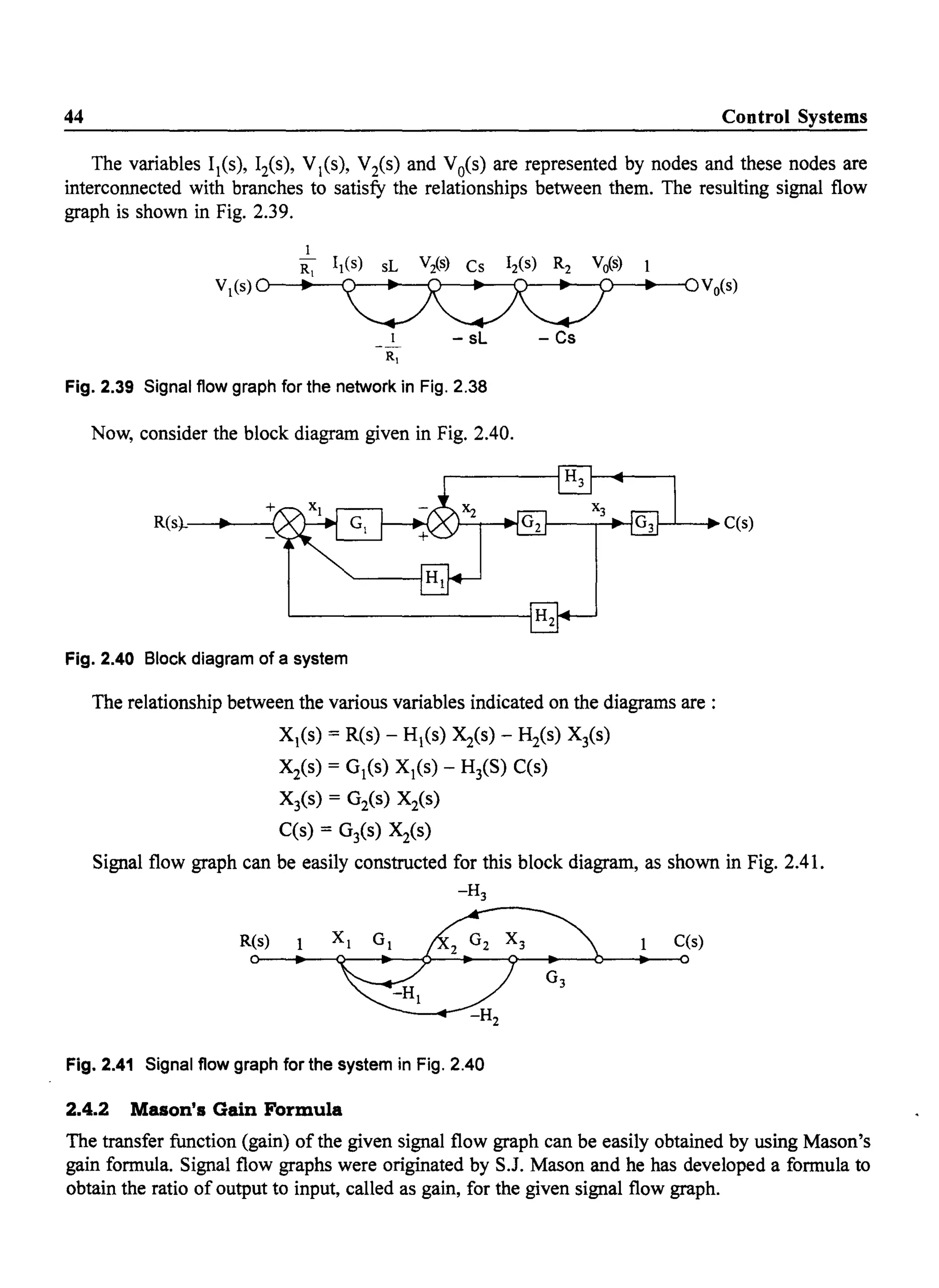
52. Mathematical Modelling of Physical Systems 43
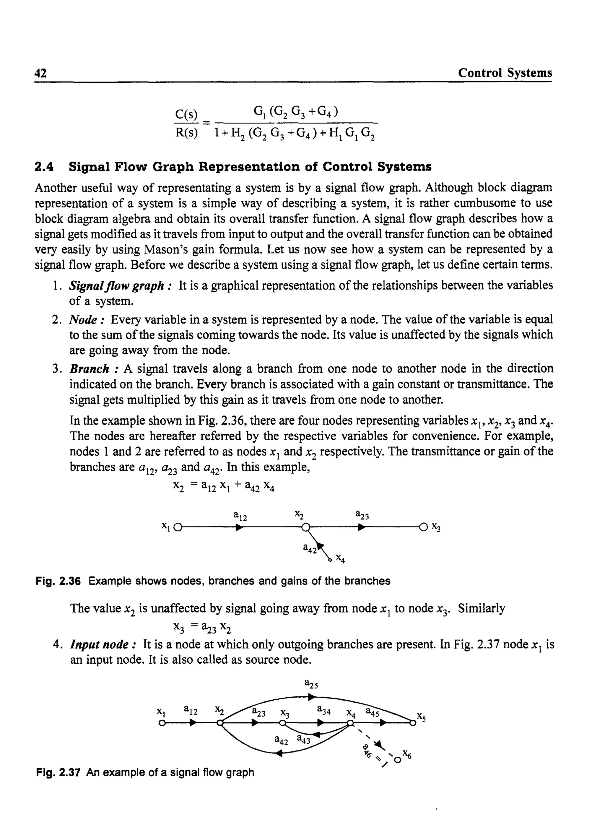
5. Output node: It is a node at which only incoming signals are present. Node Xs is an output
node. In some signal flow graphs, this condition may not be satisfied by any ofthe nodes. We
can make any variable, represented by a node, as an output variable. To do this, we can
introduce a branch with unit gain, going away from this node. The node at the end of this
branch satisfies the requirement of an output node. In the example ofFig. 2.37, if the variable
x4 is to be made an output variable, a branch is drawn at node x4 as shown by the dotted line in
Fig. (2.37) to create a node x 6. Now node x6 has only incoming branch and its gain is a46 = 1.
Therefore x6 is an output variable and since x 4 = x 6' x 4 is also an output variable.
6. Path: It is the traversal from one node to another node through the branches in the direction
of the branches such that no node is traversed twice.
7. Forward path: It is a path from input node to output node.
In the example ofFig. 2.37, Xl - x 2 - x3 - x 4 - Xs is a forward path. Similarly x l- x2 - Xs is also
a forward path
8. Loop: It is a path starting and ending on the same node. For example, in Fig. 2.37, x3 - x 4 - x3
is a loop. Similarly x 2 - x3 - x 4 - x 2 is also a loop.
9. Non touching loops: Loops which have no common node, are said to be non touching loops.
10. Forward path gain: The gain product of the branches in the forward path is calledforward
path gain.
11. Loop gain : The product of gains of branches in the loop is called as loop gain.
2.4.1 Construction of a Signal Flow Graph for a System
A signal flow graph for a given system can be constructed by writing down the equations governing
the variables. Consider the network shown in Fig. 2.38.
+
R2 Vo(s) output
Fig. 2.38 A network for constructing a signal flow graph
Identifying the currents and voltages in the branches as shown in Fig. 2.38; we have
Vis) = [Il(s) - I2(s)] sL
I2(s) = [V2(s) - Vo(s)]Cs
Vo(s) = 12(s) R2

53. 44 Control Systems
The variables 11(s), 12(s), V1(s), V2(s) and Vo(s) are represented by nodes and these nodes are
interconnected with branches to satisfy the relationships between them. The resulting signal flow
graph is shown in Fig. 2.39.
Fig. 2.39 Signal flow graph for the network in Fig. 2.38
Now, consider the block diagram given in Fig. 2.40.
R(s~-.......--( I--'--~ C(s)
Fig. 2.40 Block diagram of a system
The relationship between the various variables indicated on the diagrams are :
X1(s) = R(s) - H1(s) ~(s) - His) Xis)
X2
(s) = G1(s) X1(s) - H3
(S) C(s)
X3(s) = Gis) X2(s)
C(s) = G3(s) X2(s)
Signal flow graph can be easily constructed for this block diagram, as shown in Fig. 2.41.
-H3
R(s) C(s)
Fig. 2.41 Signal flow graph for the system in Fig. 2.40
2.4.2 Mason's Gain Formula
The transfer function (gain) of the given signal flow graph can be easily obtained by using Mason's
gain formula. Signal flow graphs were originated by S.l. Mason and he has developed a formula to
obtain the ratio of output to input, called as gain, for the given signal flow graph.

54. Mathematical Modelling of Physical Systems 45
Mason's gain fonnula is given by,
output variable 1: Mk ~k
T = input variable = k ~ .....(2.65)
where Mk is the J(h forward path gain, ~ is the detenninant of the graph, given by,
~ = 1 -1: Pml + 1: Pm2 •••••. (-ll 1: Pmr ••.••(2.66)
where Pmr is the product of the gains of mth
possible combination of r non touching loops.
or ~ = 1 - (sum of gains of individual loops) + sum of gain products of possible combinations
of 2 non touching loops) - (sum of gain products of all possible combinations of 3
nontouching loops) + ..... .....(2.67)
and ~k is the value of ~ for that part ofthe graph which is non touching with kth forward path.
To explain the use ofthis fonnula, let us consider the signal flow graph shown in Fig. 2.42, and
find the transfer function C(s)/R(s).
R(s) gl2
Fig. 2.42 Signal flow graph to illustrate Mason's gain formula
Let us enumerate the forward paths and loops of this flow graph.
1. Forwardpaths
2. Loops
MI = gl2 g23 g34 g4S gS6 g67
M2 = gl2 g23 g36 g67
M3 = gl2 g23 g34 g46
LI =g23 h32
~ = g23 g34 h42
L3 = ~s hS4
L4 = gS6 h6s
Ls = g46 h6s hS4
L6 = g23 g36 h6s hS4 h42
&7 C(s)

55. 46 Control Systems
3. Two non touching loops
Out ofthe six loops there are 3 combinations oftwo non touching loops. Their gain products are:
P12= LI L3 = g23 g4S h32 hS4
P22= LI L4 = g23 gS6 h32 h6s
P32= LI Ls = g23 g46 h32 h6s hS4
4. Three non touching loops
There is no combinations of 3 non touching loops or 4 nontouching loops etc.
.. Pm3 =Pm4 =·····O
Let us now calculate the determinant of the flow graph.
Ll = 1 - (LI + L2 + L3 + L4 + Ls + L6) + PI2 + P22 + P32
= 1- (g23 h32 + g23 g34 h42 + g4s hS4 + gS6 h6S + g46 h6s hS4
+ g23 g36 h6s hS4 h42) + (g23 g4S h32 hS4 + g23 gS6 h32 h6s
+ g23 g46 h32 h6s hs4)
and LlI = value of Ll which is non touching with MI'
Eliminate all terms in Ll which have any node in common with forward path MI' All loops LI to L6
have at least one node in common with MI and hence,
LlI = 1
Similarly Ll2 = value of Ll which is non touching with M2.
The loop L3 is not having any common node with Mz and hence eliminating all loops except L3
we have,
Ll2 = 1- L3 = 1- g4S hS4
Similarly, Ll3 = 1
Applying Mason's gain formula (eqn. 2.65) we have
C(s) M[ Ll[ + M2 Ll2 + M3 Ll3
T(s) = R(s) = Ll
Example 2.12
Vo (s)
Find the transfer function V; (s) for the network shown in Fig.2.38.
Solution: The network and its signal flow graph are reproduced in Fig. 2.43(a) and (b) for convenience.
Step 1 : Forward paths: There is only one forward path.
1
PI = - . sL. Cs. Rz
R[
LCs
2
R2
R[

56. Mathematical Modelling of Physical Systems
(a) The network
Step 2: (i) Loop gains
Fig. 2.43
L =_ Ls
I RI
~ = Cs (- sL) = - s2 LC
L3 =- ~ Cs
(ii) Product ofgains oftwo non touching loops
P12= LI.L3
sL
= - - (- R2 cs)
Rl
R2 2
= R .LCs
1
Step 3 : The determinant ofthe graph
(b) Its signal flow graph
Ls R2
Ll = 1 + _+S2 LC+R2Cs+- LCs2
RI RI
and LlI = 1
Step 4: The transfer function is
LCs
2
R2
Vo(s) _ RI
VI (s) - 1+ Ls + s2LC + R Cs + R2 LCs2
R 2 R
I I
47

57. 48 Control Systems
Example 2.13
Find the transfer function for the block diagram of Fig. 2.40.
Solution: The block diagram and its signal flow graph are reproduced in Fig. 2.44 (a) and (b).
R(s)-.......--t 1--'---' C(s)
Fig. 2.44 (a) Block diagram of a system
R(s) 0-___---0-.......-0-___---0-.......-<>--+--0 C(s)
Fig. 2.44 (b) Signal flow graph of block diagram in Fig. 2.44 (a)
Step 1 : Forward path gains
PI=GI G2 G3
Step 2: Loop gain
LI =-GIHI
L2 =-GI G2 H2
L3 =-G2 G3 H3
Two or more non touching loops are not present hence
Pmr = 0 for r = 2, 3, .....
Step 3: The determinant ofthe graph
Ll = 1 + GI HI + GI G2 H2 + G2 G3 H3
Lli = 1
Step' Transfer function

58. Mathematical Modelling of Physical Systems 49
Example 2.14
Draw the signal flow graph for the block diagram given in Fig. 2.45 (a) and obtain the transfer
function C(s)/R(s).
R(s)
Fig. 2.45 (a) Block diagram of a system
R(s) o---t_-O-__-<r---t_-o-+---o---t_-o C(s)
Fig. 2.45 (b) Signal flow graph of block diagram in Fig. 2.45 (a)
Solution: The signal flow graph can be easily written down as
Step 1 : Forwardpath gains
There are two forward paths
Step 2 : Loop gains
PI =°1° 2° 3
P2 =°1° 4
LI =-0102 HI
~ =-°2° 3H2
L3 =-°1° 2° 3
L4 =-04H2
Ls =-°1° 4
No two or more non touching loops. Hence Pmr = 0 for r = 2, 3, 4 .....
Step 3 : The determinant ofthe graph
C(s)
.( = 1 + ° 102 HI + 02 03 H2 + ° 102 0 3+ 04 H2 + ° 104
.(1 = 1
~ = 1

59. 50 Control Systems
Step 4 : The transfer function is,
C(s) G1(G2G3 + G4 )
R(s) 1+G1G2H 1 +G2G3H 2 +G1G2G3 +G1G4 +G4H2
Example 2.15
C(s) C(s)
Find the transfer function Rl (s) and R2 (s) in Fig. 2.46(a) using signal flow graph technique and
assuming that only one input is present in each case.
Fig. 2.46 (a) Block diagram of the system
Solution: The signal flow graph of the system can be easily written down as;
Fig. 2.46 (b) Signal flow graph of system in Fig. 2.46(a)
C(s)
(a) Transfer function Rl (s) ; ~ (s) = 0
Step 1: Forward path gain
Pl=G1 G2 G3
Step 2: Loop gain
Ll =-G2 H3
L2 =-G3 H2
L3 =-G1 G2 G3 H1
Two or more non touching loops are not present.
R2(s)
Pmr = 0 for r = 2, 3,4 .....
C(s)

60. Mathematical Modelling of Physical Systems
Step 3: Determinant of the graph
~ =1+G2H3+G3H2+GjG2G3Hj
~j = 1
C(s)
Step 4: Transfer function Rl (s) is given by
C(s) G1G2G3
R1(s) 1+G2H3 +G3H2 +G1G2G3H1
C(s)
(b) Transfer function R
2
(s) ; Rj(s) = 0
Step 1: Forward path gains
Pj =G3
Step 2,' Loop gains
L j =-G3 H2
L2 =-G3H j G j G2
L3 =-G2 H3
Two or more non touching loops are not present. Hence
Pmr = 0 for r = 2, 3 .....
Step 3: Determinant of the graph
L = 1 + G3H2 + G3 H j G j G2+ G2 H3
~j = 1 + G2 H3
Step 4: Transfer function C(s) is given by
R2 (s)
C(s) G3(l + G2H3 )
=-----"-'----!'--"-'----
Example 2.15
C(s)
Obtain R(s) for the signal flow graph of Fig. 2.47.
R(s)
Fig. 2.47 Signal flow graph for ex. 2.15
1 C(s)
51

61. 52
S"lution :
Step 1: Forward path gains
There are six forward paths in this graph.
PI = °1 °2 °3
P2 =OI0706
P3 =-01 07 HI Os 0 3
P4 = - 04 Os H2 07 0 6
Ps = 04 0 s 0 6
P6 = G4 Os 0 3
Step 2: Loop gains
LI =-02 H2
~ =-05 HI
L3 =07 HI 0SH2
There is one set of two non touching loops. They are LI and L2
.. P12= 02 05 HI H2
Step 3: The determinant of the graph is
Ll = 1 + 02 H2 + 0 s HI - 07 Os HI H2 + 02 0 s HI H2
LlI = (1 + HI 05)
Ll2 = Ll3 = Ll4= Ll6 = 1
Lls = 1 + H2 02
Step 4: The transfer function C(s)/R(s) is
Control Systems
01 02 0 3(1 + HI 05) + 01 07 0 6- 01 07 HI Os 0 3- 04Os H2 °7°6
C(s)
R(s)
2.5 Effects of Feedback
The output of an o~n loop system depends on the input and the parameters of the system. For the
same input, the output may be different if the parameters of the system change due to various
reasons like, variation in environmental conditions, degradation ofcomponents etc. The output is also
affected by any noise that may be present in the system. Also, if the system dynamics are to be
altered to suit the requirements, the system parameters have to be altered.
To overcome these problems, feedback can be effectively used. The output is measured by suitable
means, compared with the reference input and an actuating signal can be produced as an input to the
system, so that desired output is obtained. It means that the input to the system is continuously
changed in such a way that the system produces the required output. When the output is the desired

62. Mathematical Modelling of Physical Systems 53
output, the error signal and the actuating signal are zero. As long as this error signal is present, the
output gets modified continuously. Even if the parameters of the system change due to any reason,
the output will always tend towards the desired value. A feedback system is shown in Fig. 2.48.
output
feedback signal
Fig. 2.48 A feedback system
Let us now consider the effects of feedback on the performance of the system.
2.5.1 Effect on system dynamics
The system dynamics can be changed without actually altering the system parameters. This can be
illustrated with a simple example of a first order system. Consider the system shown in Fig. 2.49.
f--_ _ _.,--....C(s)
'-------0
Fig. 2.49 A first order system
When the switch is open, the system is an open loop system and the open loop transfer function
is given by
T(s) = C(s) = ~
R(s) s+a
The impUlse response of the system is given by h(t) = L-1T(s) = K1e-at
The time constant 't is given by
't = -
a
K
and the d.c gain (value ofT(s) when s = 0) is given by K = _I
a
The transfer function has a pole at s = -a
.....(2.67)
.....(2.68)
.....(2.69)
.....(2.70)
If the gain KI is changed by using an amplifier in cascade with the system, it cannot change the
time constant of the system. It can only alter the d.c. gain. So ifthe system speed is to be improved,
only the parameter a has to be changed.

63. S4 Control Systems
Let us now close the switch so that, the system becomes a feedback system. The closed loop
transfer function is given by,
C(s) s+a = Kl
T(s) = R(s) =l+~ -s-+-a--'-+-K-1
s+a
The impulse response of this system is, h(t) = Kj e-(a + Kj) t
The time constant and the dc gain are given by,
1
.=--a+Kl
.....(2.71)
.....(2.72)
.....(2.73)
Kl
K= a+Kl .....(2.74)
By a suitable choice ofKj , the time constant. can be altered. The system response can be speeded
up by decreasing the time constant by a suitable choice ofthe gain Kj ofthe amplifier. The pole ofthe
feedback.system is located at -(a + Kj ) and this can be pushed to the left of the jro axis to speed up
the system-as shown in Fig. 2.50.
-(a + K,)
Pole of
closed loop
system
-a
(Pole of open
loop system)
1m s
s - plane
Re s
Fig. 2.50 Poles of open loop and closed loop systems and their responses
Thus without altering the system parameter 'a' the system time constant can be adjusted to a
desired value by using an external amplifier with a suitable gain. However the d.c. gain is reduced as
given by equation 2.74. This gain can be compensidated by having additional gain outside the loop.
2.5.2 Effect due to parameter variations
The output ofan open loop system is affected by any variations in the parameter values. However, in
a closed loop system, the variations in system parameters do not change the output significantly. This
effect can be best studied by finding the sensitivity of the output to variations in system parameters.
The term sensitivity of a variable with respect to a parameter is defined as
Percentagechangein variable x
Sx = Sensitivity = .
Y Percentagechange m parameter y
.....(2.75)
.....(2.76)

64. Mathematical Modelling of Physical Systems ss
1. Sensitivi;y of overall transfer function for a small change in forward path transfer function
G(s), SG
(a) For open loop system
C(s) = G(s) R(s)
C(s)
R(s) = T(s) = G(s)
ST=OT.G=l
G
=l
G OGT ·G'
(b) For closed loop system
C(s) G(s)
- = T(s) =
R(s) 1+ G(s)H(s)
T OT G (1+GH)-GH
SG = OG·r = (1 + GH)2
l+GH
G(1+GH)
G
.....(2.77)
.....(2.78)
From eqns. (2.77) and (2.78) it is clear that the sensitivity of over all transfer function
for a small variation in forward path transfer function is reduced by a factor (1 + GH)
in a closed loop system compared to the open loop system.
2. Sensitivity ofclosed loop transfer function T(s) with respect to variation in feedback transfer
function H(s), SJ
ST
OTH
=--G oH·T
G
T(s) = - -
l+GH
ST G H(1 + GH)
G --
(1 + GH)2 G G
GH
-- .....(2.79)
l+GH
From eqn. (2.79) it is clear that for large values ofGH, the sensitivity approaches unity. Thus
the over all transfer function is highly sensitive to variation in feedback elements and therefore
the feedback elements must be properly chosen so that they do not change with environmental
changes or do not degrade due to ageing. These elements are usually low power elements and
hence high precision elements can be chosen at a relatively less cost. On the other hand, the
forward path elements need not satisfy stringest requirements, as any variations in them do
not affect the performance of the system to a significant extent. These are high power
elements and hence less precise elements at lower cost can be chosen for the forward path.

65. 56 Control Systems
Example 2.16
(a) For the open loop system in Fig. 2.51 (a) find the percentage change in the steadystate value
of C(s) for a unit step input and for a 10% change in K.
(b) For the closed loop system in Fig. 2.51 (b), find the percentage change in the steadystate
value ofC(s) for a unit step input for the same increase in the value ofK.
R(s)
I~ If----C(S) R~~I
Fig. 2.51 (a) Open loop system (b) Closed loop system'
Solution:
(a)
(b)
K
G(s) O.ls+1
C(s) = G(s) R(s)
K
s (O.ls + 1)
Lt Lt Ks
css s~O sC(s) = s~O s(O.ls+l) =K
SCss = ocss.~ = 1 K = 1
H oK css . K
.. % change in css for 10% change in K = 10%
K
T(s)
O.ls+1 +K
K
C(s)
s(O.ls + 1+ K)
K
css
=--
I+K
SCss
oCss ~
=
(l+K)I-K.l
=
OK (1+KiK css
1
I+K
10
.. % change in css for 10% change in K = 1+ K
and for K = 10
10
% change in css = U = 0.91
K(l+K)
K
C(s)

66. Mathematical Modelling of Physical Systems 57
2.5.3 Effect on Bandwidth
1
A cr.·ntrol system is essentially a low pass filter. At some friquency OJb the gain drops to J2 of its
value at OJ = o. This frequency OJb is called as the bandwidth ofthe system. Ifthe bandwidth is large,
the system response is good for high frequencies also. To put in another way, ifthe bandwidth ofthe
system is large, the speed of response is high.
K
Consider the open loop system with G(s) = --1
'ts +
At any given frequency s = jro
K
GUro) = - -
jro 't + 1
K
If ro = rob' IG Urob)1 = Ijrob't + 11
G(O)
But IG UroJI = J2 and G(O) = K
This is true if rob 't = 1
ro =-
b 't
K
Now consider a unity feedback system with G(s) = --1
'ts +
The closed loop transfer function is given by
K
T(s)- - - -
'ts+l+K
At a given frequency s = j OJ, we have
K
TUro) = 'tjro + 1+ K
K
IT (Grob)1 = l'tjrob + 1+ KI
T(O) 1 K
TUrob) = J2 = J2·1 + K
This is true if, rob 't = 1 + K
I+K
.....(2.80)
or rob = -'t- .....(2.81)
From eqns. (2.80) and (2.81) it is clear that the bandwidth ofclosed loop system is (1 + K) times
the bandwidth of open loop system. Hence the speed of response of a closed loop system is larger
than that of an open loop system.

67. 58 Control Systems
2.5.4 Effect on Noise Signals
(a) Noise in the forward paths
Consider the block diagram of the system shown in Fig. 2.52.
N(s)
R(s) =0 + C(s)
'---------i H(s) 1+--------'
Fig. 2.52 Noise in the forward path
A noise signal is added between the forward path blocks Gt(s) and G2(s). To evaluate the effect of
N(s), we assume R(s) = O. The transfer function between C(s) and N(s) can be easily derived as,
C(s) G2 (s)
TN(s) = N(s) =1+GI(s)G2(s)H(s)
For the practical case of IGt(s) Gis) H(s)1 » 1
1
TN(s) = GI(s) H(s)
or
N(s)
C(s) = GI(s) H(s) .....(2.81)
It can be seen from eqn. (2.81) that the effect of noise on output can be reduced by making
I(GI(s)1 sufficiently large.
(b) Noise in feedback path
Consider the block diagram in Fig. 2.53.
R(s) =0 + C(s)
Fig.2.53 Noise in the feedback path
The transfer function between output and the noise signal with R(s) = 0 is given by
C(s) -G(s)H2(s)
T(s) = N(s) = 1+ G(s) HI (s) H2 (s)
For IG(s) HI(s) ~(s)1 » 1, we have
1
T(s) = - HI(s)
1
and C(s) = - HI (s) N(s)
Thus by making HI(s) large the effects of noise can be effectively reduced.

68. Mathematical Modelling of Physical Systems 59
2.6 Modelling of Elements of Control Systems
A feedback control system usually consists of several components in addition to the actual process.
These are: error detectors, power amplifiers, actuators, sensors etc. Let us now discuss the physical
characteristics of some of these and obtain their mathematical models.
2.6.1 DC Servo Motor
A DC servo motor is used as an actuator to drive a load. It is usually a DC motor oflow power rating.
DC servo motors have a high ratio of starting torque to inertia and therefore they have a faster
dynamic response. DC motors are constructed using rare earth permanent magnets which have high
residual flux density and high coercivity. As no field winding is used, the field copper losses are zero
and hence, the overall efficiency of the motor is high. The speed torque characteristic of this motor
is flat over a wide range, as the armature reaction is negligible. Moreover speed is directly proportional
to the armature voltage for a given torque. Armature of a DC servo motor is specially designed to
have low inertia.
In some application DC servo motors are used with magnetic flux produced by field windings.
The speed ofPMDC motors can be controlled by applying variable armature voltage. These are called
armature voltage controlled DC servo motors. Wound field DC motors can be controlled by either
controlling the armature voltage or controlling the field current. Let us now conside'r modelling of
these two types of DC servo motors.
(a) Armature controlled DC servo motor
The physical model of an armature controlled DC servo motor is given in Fig. 2.54.
If = Const
e, J, Bo EFig. 2.54 Armature controlled DC servo motor.
The armature winding has a resistance Ra and inductance La' The field is produced either by a
permanent magnet or the field winding is separately excited and supplied with constant voltage so
that the field current If is a constant.
When the armature is supplied with a DC voltage of ea volts, the armature rotates and produces a
back e.m.f eb• The armature current ia depends on the difference of ea and eb. The armature has a
moment of inertia J, frictional coefficient Bo' The angular displacement of the motor is e.
The torque produced by the motor is given by,
T = KT ia
where KT is the motor torque constant.
.....(2.84)

69. 60
The back emf is proportional to the speed of the motor and hence
eb=Kb 9
The differential equation representing the electrical system is given by,
di
R . +L a + -a la a dt eb- ea
Taking Laplace transform of eqns. (2.84), (2.85) and (2.86) we have
T(s) = KT laCs)
Eb(s) = Kb s 9(s)
(Ra + s La) laCs) + Eb(s) = Ea(s)
I (s) = Ea (s) - KbS 9(s)
a Ra +sLa
The mathematical model ofthe mechanical system is given by,
d29 d9
J - + Bo- =T
dt2 dt
Taking Laplace transform of eqn. (2.91),
(Js2 + Bos) 9(s) = T(s)
Using eqns. (2.87) and (2.90) in eqn. (2.92), we have
Ea (s) - KbS 9(s)
9(s) = KT (Ra + sLa)(Js2 + Bos)
Solving for 9(s), we get
9(s) = KT Ea (s)
s[(Ra +sLa)(Js+BO)+KT Kb]
Control Systems
.....(2.85)
.....(2.86)
.....(2.87)
.....(2.88)
.....(2.89)
.....(2.90)
.....(2.91)
.....(2.92)
.....(2.93)
.....(2.94)
The block diagram representation of the armature controlled DC servo motor is developed in
steps, as shown in Fig. 2.55. Representing eqns. (2.89), (2.87), (2.92) and (2.88) by block diagrams
respectively, we have
(ii)
(iii) (iv)
Fig. 2.55 Individual blocks of the armature controlled DC servo motor.

70. Mathematical Modelling of Physical Systems 61
Combining these blocks suitably we have the complete block diagram as shown in Fig. 2.56.
Fig. 2.56 Complete block diagram of an armature controlled DC servo motor
Usually the inductance ofthe armature winding is small and hence neglected. The overall transfer
function, then, becomes,
Kr IRa
s(Js + B)
where B = Bo + KbKr is the equivalent frictional coefficient.
Ra
.....(2.95) .
.....(2.96)
It can be seen from eqn. (2.95) that the effect of back emf is to increase the effective frictional
coeffcient thus providing increased damping. Eqn. (2.96) can be written in another useful form
known as time constant form, given by,
.....(2.97)
where
K
KM = R r
J
is the motor gain constant
a
and J . h .
"m = B IS t e motor tIme constant
(Note: Kb and KT are related to each other and in MKS units Kb = KT. Kb is measured in V/rad/sec
and KT is in NmlA)
Armature controlled DC servo motors are used where power requirements are large and the
additional damping provided inherently by the back emf is an added advantage.

71. 62
(b) Field controlled DC servo motor
The field controlled DC servo motor is shown in Fig. 2.57.
~
+
Fig. 2.57 Field controlled DC servo motor
The electrical circuit is modelled as,
lis) = Ef(s)
Rf +Lfs
T(s) = KT Ir(s)
and (Js2 + Bo) 9(s) = T(s)
Combining eqns. (2.98), (2.99) and (2.100) we have
where
9(s) Kr
Ef(s) s(Js + Bo)(Rf + Lfs)
s('tms + l)('tfs + 1)
~ = KTfR.;30 = motor gain constant
'tm = JlBo = motor time constant
1- = L/Rt-= field time constant
The block diagram i~ as shown in Fig. 2.58.
Fig. 2.58 Block diagram of a field controlled DC servo motor
Ia = Const
Control Systems
.....(2.98)
.....(2.99)
.....(2.100)
.....(2.101)
Field controlled DC servo motors are economcial where small size motors are required. For the
field circuit, low power servo amplifiers are sufficient and hence they are cheaper.

72. Mathematical Modelling of Physical Systems 63
2.6.2 AC Servo Motors
An AC servo motor is essentially a two phase induction motor with modified constructional features
to suit servo applications. The schematic of a two phase ac servo motor is shown in Fig. 2.59.
Control r-Vr1
o-____~----~__~wm~·=d~mg ~
Actuation
signal
Servo
amplifier
Fig. 2.59 Schematic of a 2 phase ac servo motor
Reference
windmg
It has two windings displaced by 90° on the stator. One winding, called as reference winding, is
supplied with a constant sinusoidal voltage. The second winding, called control winding, is supplied
with a variable control voltage which is diplaced by ± 90° out of phase from the reference voltage.
The major differences between the normal induction motor and an AC servo motor are:
1. The rotor winding of an ac servo motor has high resistance (R) compared to its inductive
reactance (X) so that its ~ ratio is very low. For a normal induction motor, ~ ratio is high
so that the maximum torque is obtained in normal operating region which is around 5% ofslip.
The torque speed characteristics of a normal induction motor and an ac servo motor are
shown in Fig. 2.60.
Torque
Synchronous
speed
Speed
Fig. 2.60 Torque speed characteristics of normal induction motor and ac servo motor
The Torque speed characteristic of a normal induction motor is highly nonlinear and has a
positive slope for some portion of the curve. This is not desirable for control applications, as
the positive slope makes the systems unstable. The torque speed characteristic of an ac servo
motor is fairly linear and has negative slope throughout.
2. The rotor construction is usually squirrel cage or drag cup type for an ac servo motor. The
diameter is small compared to the length of the rotor which reduces inertia of the moving
parts. Thus it has good accelerating characteristic and good dynamic response.
3. The supply to the two windings of ac servo motor are not balanced as in the case of a normal
induction motor. The control voltage varies both in magnitude and phase with respect to the
constant reference voltage applied to the reference winding. The direction of ratation of the
motor depends on the phase C± 90°) ofthe control voltage with respect to the reference voltage.

73. 64 Control Systems
For different rms values of control voltage the torque speed characteristics are shown in
Fig. 2.61. The torque varies approximately linearly with respect to speed and also _control
voltage. The torque speed characteristics can be linearised at the operating point and the transfer
function 9f the motor can be obtained.
Speed 8
Fig. 2.61 AC servo motor speed torque characteristics
The torque is a function of speed a and the control voltage E. Thus
TM = f(a, E) .....(2.102)
Expanding eqn. (2.102) in Taylor series around the operating point, TM= TMO' E = Eo and a = a 0
and neglecting terms of order equal to and higher than two, we have
OTMI ( ) OTMI ..TM=TMO + BE ?=Eo E-Eo + oe ?=Eo(8-80 )
9=9 9=9
o 0
or
where
(Note: Since OT~ is negative, B will be positive)
oe
Eqn. (2.104) can be written as
~TM=KAE-B~a
The mechanical equation is given by
J ~e +Bo~a =~TM=~-B~a
.....(2.103)
.....(2.104)
.....(2.105)
.....(2.106)
.....(2.107)
Taking Laplace transform of eqn. (2.107), we get the transfer function of an ac servo motor as,
~8(s) K
- - = ---:::-----
~E(s) Js2
+ (Bo + B)s
.....(2.108)
In time constant form we can write eqn. (2.108) as
.....(2.109)

74. Mathematical Modelling of Physical Systems 65
where TC K M .'''m = = otor gam constant
Bo +B
J
and "em = Bo + B = Motor time constant
Ifthe slope of the torque speed characteristic is positive, B, from eqn. (2.105) is negative and the
effective friction coefficient Bo + B may become negative and the system may become unstable.
The transfer function of the motor around the op.erating point may be written as,
C(s)= 9(s) = Km ......(2.110)
E(s) s("ems +1)
The constants K and B can be obtained by conducting a no load test and blocked rotor test on the
ac servo motor at the rated control voltage Ec.
On no load TM = 0 and on blocked rotor, e= o.
These two points are indicated as P and Q respectively on the diagram of Fig. 2.62. The line
joining P and Qrepresents the approximate speed torque characteristic at rated control voltage.
p
torquei
Q
o Speed e-.
Fig. 2.62 Torque speed characteristic of servo motor at rated control voltage
and
T
B = ---¥-
9
.....(2.111 )
.....(2.112)
To take into effect the nonlinearity of the torque speed curve, B is usually taken to be half of the
value given by eqn. (2.112).
2.6.3 Synchros
A commonly used error detector of mechanical positions of rotating shafts in AC control systems is
the Synchro. It consists of two electro mechanical devices. 1. Synchro transmitter 2. Synchro
receiver or control transformer. The principle of operation of these two devices is same but they
differ slightly in their construction.
The contruction of a Synchro transmitter is similar to a 3 phase alternator. The stator consists of
a balanced three phase winding and is star connected. The rotor is ofdumbbell type -construction and

75. 66 Control Systems
is wound with a coil to produce a magnetic field. When an ac voltage is applied to the winding ofthe
rotor, a magnetic field is produced. The coils in the stator link with this sinusoidally distributed
magnetic flux and voltages are induced in the three coils due to transformer action. Thus the three
voltages are in time phase with each other and the rotor voltage. The magnitudes of the voltages are
proportional to the cosine of the angle between the rotor position and the respective coil axis. The
position of the rotor and the coils are shown in Fig. 2.63.
S2
..... e+ 2400
"" ".f'"n e+ 1200
¥
AC supply
,I
~---------------------o
Fig. 2.63 Synchro transmitter
If the voltages induced in the three coils are designated as Vs ,vs and Vs and if the rotor ltXis
makes angle Bwith the axis of SI winding, we have, 1 2 3
vR(t) = vr Sin ffirt
Vs = KVr Sin ffirt cos (9 + 120)
In
v~n = KVr Sin ffirt cos 9
Vs = KVr Sin ffirt cos (9 + 240)
3n
These are the phase voltages and hence the line voltages are given by,
vSls2 = vsln - v~n = J3 KVr Sin (9 + 240) Sin ffirt
v~s3 =vs2n-vs3n= J3 KVr Sin (9 + 120)Sinffirt
.....(2.113)
.....(2.114)
.....(2.115)
.....(2.116)
.....(2.117)
vS3S1 = VS3n- VSIn= J3 KVr Sin eSin ffirt .....(2.118)
When B= 0, the axis ofthe magnetic field coincides with the axis ofcoil S2 and maximum voltage
is induced in it as seen from eqn. (2.114). For this position of the rotor, the voltage Vs s is zero, as
given by eqn. (2.118). This position of the rotor is known as the 'Electrical Zero' of trleransmitter
and is taken as reference for specifying the rotor position.
In summary, it can be seen that the input to the transmitter is the angular position ofthe rotor and
the set of three single phase voltages is the output. The magnitudes of these voltages depend on the
angular position of the rotor as given in eqn. (2.116) to (2.118).
Now consider these three voltages to be applied to the stator of a similar device called control
transformer or synchro receiver. The construction of a control transformer is similar to that of the
transmitter except that the rotor is made cylindrical in shape whereas the rotor of transmitter is

76. Mathematical Modelling of Physical Systems 67
dumbell in shape. Since the rotor is cylindrical, the air gap is uniform and the reluctance of the
magnetic path is constant. This makes the output impedance of rotor to be a constant. Usually the
rotor winding ofcontrol transformer is connected to an amplifier which requires signal with constant
impedance for better performance. A synchro transmitter is usually required to supply several control
transformers and hence the stator winding of control transformer is wound with higher impedance
per phase.
Since the same currents flow through the stators of the synchro transmitter and receiver, the
same pattern of flux distribution will be produced in the air gap of the control transformer. The
control transformer flux axis is in the same position as that of the synchro transmitter. Thus the
voltage induced in the rotor coil of control transformer is proportional to the cosine of the angle
between the two rotors. Hence,
elt) = K, Vr Cos <I> sin rort .....(2.119)
where ¢ is the angle between the two rotors. When ¢ = 90°, e/t) = 0 and the two rotors are at right
angles. This position is known as the 'Electrical Zero' for the control transformer. In Fig. 2.64, a
synchro transinitter receiver pair (usually called Synchro pair) connected as an error detector, is
shown in the respective electrical zero positions.
Fig. 2.64 Synchro pair connected as error detector
If the rotor of the transmitter rotates through an angle 8 in the anticlockwise direction, and the
rotor of control transformer rotates by an angle a. in the anticlockwise direction, the net angular
displacement between ~he two is (90 - 8 + a.). From eqn. (2.119),
elt) = K, Vr Sin rort Cos (90 - 8 + a.)
= K, Vr Sin (8 - a.) Sin rort
If «()- a) is small, which is usually the case,
elt) = K, Vr (8 - a.) Sin rort
.....(2.120)
.....(2.121)
Thus the synchro pair acts as an error detector, by giving a voltage elf) proportional to the
difference in the angles ofthe two rotors. Ifthe angular position of synchro transmitter is used as the
reference position, the transformer rotor can be coupled to the load to indicate the error between the
reference and the actual positions.

77. 68 Control Systems
The waveform oferror voltage for a given variation ofdifference in the angular positions together
with the reference voltage is shown in Fig. 2.65.
v(t)
(8 - a)
Fig. 2.65 Waveforms of voltages in synchro error detector
Thus, we see that the output of the error detector is a modulated signal with the ac input to the
rotor of transmitter acting as carrier wave. The modulating signal em(t) is
ern(t) = Ks (9 - a) .....(2.122)
where ~ is known as the sensitivity of the error detector. Thus the synchro pair is modelled by the
eqn. (2.122) when it is connected as an error detector.
2.6.4 AC Tacho Generator
An ac tacho generator consists of two coils on the stator displaced by 900
• The rotor is a thin
aluminium cup that rotates in the air gap in the magnetic flux produced by one of the stator coils
called as reference coil. This coil is supplied with a sinusoidal voltage, Vr Sin OJct, where OJc is called
the carrier frequency. The aluminium cup has low inertia and high conductivity and acts as a short
circuited rotor. Because of the special construction ofthe rotor, this generator is also known as drag
cup generator. The schematic of an ac tachometer is shown in Fig. 2.66.
Fig. 2.66
Refer~nce ~inooct
coli ~
drag cup Grotor~
quadrature coil
(a) Schematic of AC tacho generator
~r
(b) Ferrari's principle
The voltage applied to the reference winding produces a main flux of (A COS OJ/. As per Ferrari's
principle, this alternating flux can be considered as equivalent to two rotating fluxes ¢I and ¢h' These
two fluxes are equal in magnitude but rotating in opposite directions with synchronous speed of OJs'

78. Mathematical Modelling of Physical Systems 69
If the rotor is stationary, these two fluxes induce equal and opposite voltages in the quadrature
winding on the stator and therefore th~ voltage across this winding is zero. The two fluxes also
produce induced currents in the drag cup which in tum produce reaction fluxes oppositing the
corresponding main fluxes, resulting in the net fluxes ¢fand ¢b'
Now let the rotor rotate with a speed ein the direction of the forward flux ¢j" Since the relative
speed of rotor conductors decreases, the induced currents decrease and therefore the main forward
flux ¢f increases. The relative speed of rotor conductors increases with respect to backward flux ¢b
and the induced current in the rotor due to this flux increases. Thi~ increases the reaction flux thereby
decreasing backward flux ¢b' This imbalance in the fields, produces a voltage across the quadrature
coil. This voltage will be in phase quadrature with the reference voltage and its amplitude is
proportional to the speed of the rotor. If the rotor rotates in the opposite direction, reverse action
takes place. Thus the voltage across the quadrature coil is given by,
.....(2.123)
Ifthe speed varies slowly with respect to the frequency ofthe reference voltage, eqn. (2.123) still
applies. Thus,
Vf(t) = ~ e(t) Cos wct
The magnitude ofthis voltage is given by
vt(t) = ~ e(t)
.....(2.124)
.....(2.125)
where ~ is called the tachometer constant. Thus the ac tachometer which is generally used as a
feedback element can be modelled as a proportional element and can be represented by the block
diagrams (Fig. 2.67).
tl (t)
Fig. 2.67 Block diagram of an ac tacho meter
2.6.5 DC Tacho Generator
A DC tacho generator is used to feedback a voltage proportional to the speed in a DC control system.
The construction of a DC tacho generator in simiar to a DC permanent magnet generator. The power
rating of such a generator is very small and is designed to have low inertia.
2.6.6 Potentiometers
These devices are used commonly as feedback elements or error detectors. This is a highly reliable
device used for measuring linear motion or angular motion. A potentiometer is a resistance with three
terminals (Fig. 2.68 (a». Areference voltage is applied to the two fixed terminals. The voltage between
a movable terminals and one ofthe fixed terminals is an indication ofthe linear or angular displacement
ofthe movable terminal. The total resistance ofthe potentiometer is uniformly distributed linearly for
translatory motion or in helical form for rotatory motion. The output voltage is linearly related to the
position ofthe movable arm as long as this voltage is connected to a device with high input resistance.

79. 70 Control Systems
Otherwise loading effect will cause nonlinearity in the characteristic of the potentiometer as shown
in Fig. 2.68 (b).
Fig. 2.68 (a) Potentiometer
without loading
1.0
with loading
Fig. 2.68 (b) Effect of loading of a potentiometer
Potentiometer as an error detector.
Two resistors connected in parallel and supplied from a reference voltage with two movable
terminals can be used as an error detector as shown in Fig. 2.69.
Ref position Load position
To amplifier
Fig. 2.69 Potentiometer as an error detector
One variable arm is used for setting the reference position or desired position. The second variable
arm is connected to the load. When the position of the load is same as the reference position the
voltage applied to the amplifier is zero. If the position of the load changes, the voltage between the
two movable terminars will be non zero and this will be applied to the amplifier. Either positive or
negative errors can be detected.

80. Mathematical Modelling of Physical Systems 71
2.6.7 Stepper Motors
These motors are also called as stepping motors or simply step motors. This motor can be considered
as an electromagnetic incremental actuator which converts electrical pulses into mechanical rotation.
Stepper motors are used in digitally controlled position control systems. The input is a train ofpulses.
One advantage ofstepper motor is that it does not require position or speed sensors, as this information
can be directly obtained by counting the input pulses.
Depending on the principle of operation, there are two most common types of stepper motors.
1. Variable reluctance motor (VR motor) and
2. Permanent magnet motor (PM motor).
Variable reluctance motor
A VR motor has a wound stator and an unexcited rotor. A typical VR motor is shown in Fig. 2.70.
This is a three phase stator with twelve stator teeth. For each phase there are four teeth distributed
over the periphery of the stator and a winding is placed on these slots. The teeth are marked ABC
and windings are not shown in the diagram. The rotor has eight teeth. Both the stator and rotor are
constructed with high permeability material like silicon steel to allow large magnetic flux.
The principle of operation of VR motor is as follows. If anyone phase is excited (say A phase),
the rotor will align itself such that its teeth are directly under the teeth of excited winding so that the
reluctance of the magnetic path is low. In this position the rotor is in stable equilibrium. Now if a
pulse is given to the next phase (say B phase), the rotor teeth nearest to the B phase stator teeth will
be pulled to align directly under B phase teeth. Thus the rotor moves one step in the anticlock wise
direction. If now a pulse is given to the A phase, the rotor moves one more step in the counter
clockwise direction. If the sequence of phases to which pulses are given is altered ie from ABC to
A C B, the motor rotates in clockwise direction.
Fig. 2.70 Variable reluctance stepper motor
360
When a tooth of rotor is aligned with say, phase A, the next tooth on the rotor is 8 = 45° away
360
from it. The tooth corresponding to the next phase ie phase B is at an angle of 12 =30° from phase A.

81. 72 Control Systems
Hence when phase B is excited, the tooth on the rotor nearest to the tooth corresponding to B phase
is 45 - 30 = ISO away from it and therefore the rotor rotates through 15° in one step. So for
every pulse the rotor rotates by ISO, either in clockwise direction or anticlockwise direction depending
on the sequence of excitation of the three phases. The angle throgh which the rotor moves for one
pulse is known as the step angle. The frequency of pulses applied to the stator windings will control
the speed of rotation of the stopper motor.
Permanent Magnet motor (PM motor)
In permanent magnet motors, the rotor is made up offerrite or rare earth material and is permanently
magnetised. In the 4 pole, 2 phase PM motor shown in Fig. 2.71 the stator consists of two stacks,
each with a phase winding, displaced electrically by 90°. By exciting these two phases, phase a and
phase b suitably, stepping action can be obtained. This is shown in Fig. 2.71.
(a) (b)
Fig. 2.71 (a) Phase a of a PM motor (b) Phase b of a PM motor
Let us suppose that the phase a is given a pulse so that the stator poles are as indicated in
Fig. 2.71 (a). The rotor will align itself in the position shown in Fig. 2.71 (a). Now let us excite the
phase b also by a pulse, the stator poles effectively shift counter clockwise by 22.5° as shown in
Fig. 2.71 (b). Since the magnetic axis is shifted, the rotor also has to move by 22.So in counter
clockwise direction to align itself with the new magnetic axis. Now if phase a is unenergised, the
stator magnetic axis moves by another 22.5° in the counter clockwise direction and hence the rotor
also moves by the same angle in the same direction. To move another step in the same direction,
phase a is given a pulse in the opposite direction. Rotation in the clockwise direction can be obtained
by suitably modifying the switching scheme. Generally, two coils are provided for each phase to
facilitate easy switching by electronic circuitry.

82. Mathematical Modelling of Physical Systems
Problems
2.1 Obtain the transfer function for the following networks.
3
0
+ +
VI(S)
Cs
2 R 4
T(s) = V2(s)
VI(S)
Fig. P 2.1 (a)
2.2 Obtain the transfer functions for the following mechanical translational systems.
X2(s)
T(s) = F(s)
Fig. P 2.2 (a)
Yes)
T(s) = - -
Xes)
Fig. P 2.2 (b)
Xes)
T(s) = F(s)
Fig. P 2.2 (c)
2.3 Obtain the transfer function for the following mechanical rotational system.
Fig. P2.3
73
20

83. 74 Control Systems
2.4 Draw F - v and F - i analogous circuits for the problem 2.2 (a), (b) and (c).
2.5 Obtain the transfer function Xes) for the electromechanical system shown in Fig P 2.5.
Yes)
R
v
dx
Plunger
9---..
e 9-_~Coi1
Fig. P2.5
x
Assume e = Kb dt and the force produced on the mass f = kri.
2.6 In the thermal system shown, heater coil is used to heat the liquid entering the insulated tank
at temperature 9ito hot liquid at temperature 9. The liquid is thoroughly mixed to maintain
uniform temperature ofthe liquid in the tank. IfM is the mass ofthe liquid in the tank in Kg,
C is the specific heat of liquid in J I Kg 10K
, W is the steady state liquid flow rate in kg/sec
and hi is the heat input rate in J/sec, obtain the transfer function of the system when,
(i) Heat input rate is changed, with inlet temperature ofliquid kept constant and
(ii) inlet temperature is changed with heat input rate held constant. Also write the differential
equation when heat input rate and inlet liquid temperature are charged.
Fig. P2.6

84. Mathematical Modelling of Physical Systems 75
,
2.7 A thin glass bulb mercury thermometer is immersed suddenly in a hot both of temperature
ab
• Obtain expression for the temperature of the thermometer.
Fig. P2.7
Thermal capacitance of thermometer is C
Thermal resistance of the thermometer is R
2.8 Obtain the transfer function C(s)/ M(s) for the liquid manometer system shown in Fig P 2.8
pre~ure ~
dampingB
(Fluid density y, Area oftube A)
Fig. P2.8
2.9 Obtain the transfer function ofthe liquid level system shown in Fig. P 2.9. The output is the
liquid level c in the second vessel and the input is the inflow m.
c
Fig. P2.9

85. 76 Control Systems
2.10 A d.c position control system consists of a permanent magnet armature controlled d.c
srevomotor, a potentiometer error detector, a d.c Amplifier and a tachogenerator coupled to
the motor. Assuming the motor and load frictions to be negligible and a fraction K of the
tachogenerator output is fedback, draw the schematic of the control system and obtain its
transfer function.
The parameters of the system are,
Moment of inertia of motor, JM
= 3 x 10-3 kg - m2
Moment of inertia ofload, JL
= 4 kg - m2
Motor to load gear ratio
Load to potentiometer gear ratio
Motor torque constant
Tachogenerator constant
Sensitivity of error detector
Amplifier gain
€-.-=-
8M 50
8L
-. = 1
8e
Kt
= 2.5 Nco m I Amp
~ = 0.1 V/rad/sec
Kp = 0.5 V/rad
KAAmpsNolt
2.11 A position control system using a pair ofsynchros and an armature controlled dc servomotor
is shown in Fig. P 2.11. The demodulator has a transfer function given by Kd
. d.c volts/a.c volts.
Fig. P 2.11

86. Mathematical Modelling of Physical Systems
The sensitivity of error detector is Ks.v/rad
Draw (a) The block diagram
77
(b) The signal flow graph of ofthe system and obtain its transfer function. Use the
following values for the parameters.
Kd = 0.5 VIV
Ks = SOV/rad
KA = 10VIV
The back emf constant Kb = 1.5 VIrad/sec
KT = 1.5 Nw mlA
= 0.5 Kgm2
BL = 1 Nro/rad/sec.
Ra = In
2.12 Reduce the block diagram shown in Fig. P 2.12 and obtain the over all transfer function.
R(s) C(s)
Fig. P 2.12
2.13 Obtain the overall transfer functions for the following signal flow graphs using mason's
gain formula.
(a) R(s) o--"--o--~--<:>---+---<>---J_-o-_,,----<)--~_-o--"--oC(s)
-1
(b)
Fig. P 2.13

87. 78 Control Systems
2.14 Reduce the block diagrams shown in Fig P 2.14 and obtain theirtransfer functions.
R(s) C(s)
~--------~Hl~------------------------~
(a)
R(s) +
R(s) C(s)
(c)
Fig. P.2.14
2.15 Draw the signal flow graph for the network shown and obtain its transfer function,
12 (s)
T(s) = VIes)
1
-F
2 In
2H
IF
Fig. P 2.15
2n
IH

88. Mathematical Modelling of Physical Systems 79
2.16 Draw the signal flow graphs of the systems given in problem 2.13 and obtain their transfer
functions.
2.17 Consider the voltage regulator shown in Fig. P 2.17.
Amplifier
KA
~= 1500
s
Fig.P2.17
R.= 0.50
A voltage of KVo is fedback to the amplifier. The amplifier gain KA = 10V/volt and the
generator constant Kg = SOV/Amp.
(a) With switch S open, what should be the reference voltage to get an output voltage of
200V on no load. If the same reference voltage is maintained, what will be the output
voltage when the generator delivers a steady current of 20A.
(b) With reference voltage of 80V and switch S closed what part of the output voltage is to
be fedback to get a steady terminal voltage of 10V on no load.
(c) With the system as in part b, if the generator supplies a load of 20A, what will be the
terminal voltage.
(d) What should be the reference voltage to maintain an output voltage of200V at 20A load
under closed loop condition.
2.18 For the system shown in Fig P 2.18 determine the sensitivity of the closed loop transfer
function with respect to G, Hand K. Take ro = 2 rad/sec.
R(s) + 1 C(s)
G(s) = - - h , - - - -
s(s+2)
Fig. P.2.18

89. 80 Control Systems
2.19 In the position control system shown in Fig P. 2.19, derivative error compensation is used.
Find the sensitivity of the closed loop transfer function at (j) = lrad/sec with respect to the
derivative error coefficient Kd with nominal value of Kd = 2
R(s) + C(s)
Fig. P. 2.19
2.20 The torque speed characteristic of a two phase ac servo motor is as shown in Fig P. 2.20
with rated control voltage of IISV at 50Hz applied to the control winding. The moment of
Inertia of the motor is 7.5 x 10--{) kg-m2. Neglecting the friction of the motor, obtain its
transfer function 8(s) where 8(s) is the shaft position and Vc(s) is the control voltage.
Vc(s)
0.1
Torque in
Nw.m
1500 Speed in RPM
Fig. P.2.20
-jJ-

90. 3 Time Response Analysis of
Control Systems
3.1 Introduction
The first st~p in the analysis ofa control system is, describing the system in terms ofa mathematical
model. In chapter 2 we have seen how any given system is modelled by defining its transfer function.
The next step would be, to obtain its response, both transient and steadystate, to a specific input. The
input can be a time varying function which may be described by known mathematicalfunctions or it
may be a random signal. Moreover these input signals may not be known apriori. Thus it is customary
to subject the control system to some standard input test signals which strain the system very severely.
These standard input signals are : an impulse, a step, a ramp and a parabolic input. Analysis and
design of control systems are carried out, defining certain performance measures for the system,
using these standard test signals.
It is also pertinent to mention that any arbitary time function can be expressed in terms of linear
combinations of these test signals and hence, if the system is linear, the output of the system can be
obtained easily by using supersition principle. Further, convolution integral can also be used to determine
the response of a linear system for any given input, if the response is knownfor a step or an impulse
input.
3.2 Standard Test Signals
3.2.1 Impulse Signal
An impulse signal is shown in Fig. 3.1.
f(t)
(A)
--.t
Fig. 3.1 An Impulse signal.

91. 82 Control Systems
The impulse function is zero for all t ;t! 0 and it is infinity at t = O. It rises to infinity at t = 0- and
comes back to zero at t = 0+ enclosing a finite area. Ifthis area is A it is called as an impulse function
of strength A. If A = 1 it is called a unit impulse function. Thus an impulse signal is denoted by
f(t) = A 8 (t).
3.2.2 Step Signal
A step signal is shown in Fig. 3.2.
Af--------
f(t)
o ~t
Fig. 3.2 A Step Signal.
It is zero for t < 0 and suddenly rises to a value A at t = 0 and remains at this value for t > 0: It is
denoted by f(t) = Au (t). IfA = 1, it is called a unit step function.
3.2.3 Ramp signal
A ramp signal is shown in Fig. 3.3.
A
f(t)
1.0 ~t
Fig. 3.3 A Ramp Signal.
It is zero for t < 0 and uniformly increases with a slope equal to A. It is denoted byf (t) = At.
If the slope is unity, then it is called a unit ramp signal.
3.2.4 Parabolic signal
A parabolic signal is shpwn in Fig. 3.4.
Fig. 3.4 A unit parabolic signal.
A
2
f(t)
1.0 ~t

92. Time Response Analysis of Control Systems 83
At2
A parabolic signal is denoted byf (t) == 2' If A is equal to unity then it is known as a unit
parabolic signal.
It can be easily verified that the step function is obtained by integrating the impulse function from
o to 00; a ramp function is obtained by integrating the step function and finally the prabolic function
is obtained by integrating the ramp function. Similarly ramp function, step function and impulse
function can be to obtained by successive differentiations of the parabolic function.
Such a set of functions which are derived from one another are knowp. as singularityfunctions. If
the response ofa linear system is known for anyone ofthese input signals, the response to any other
signal, out ofthese singularity functions, can be obtained by either differentiation or integration ofthe
known response.
3.3 Representation of Systems
The input output description of the system is mathematically represented either as a differential
equation or a transfer function.
The differential equation representation is known as a time domain representation and the transfer
function is said to be a frequency domain representaiton. We will be considering the transfer function
representation for all our analysis and design of control systems.
The open loop transfer function of a system is represented in the following two forms.
1. Pole-zero form
G(s)==K (s+z,)(S+z2)···(s+zm)
I (s+P,)(s+P2) ... (s+Pn)
Zeros occur at s == -zl' -~, - - -, -~
Poles occur at s == -PI' - P2' - - -, -Pm
.....(3.1)
The poles and zeros may be simple or repeated. Poles and zeros may occur at the origin. In the
case where some of the poles occur at the origin, the transfer function may be written as
K, (s + z,)(s + Z2)"'(S + zm)
G(s) == -r----'--'--'-'--'--"-'----'---"'-'--
S (s+Pr+,)(s+Pr+2) ... (s+Pn)
.....(3.2)
The poles at the origin are given by the term ~. The term ! indicates an integration in the
sr s
1
system and hence - indicates the number of integrations present in the system. Poles at
sr
origin influence the steadystate performance of the system as will be explained later in this
chapter. Hence the systems are classified according to the number of poles at the origion.
If r == 0, the system has no pole at the origin and hence is known as a type - °system.
Ifr == 1, there is one pole at the origin and the system is known as a type - 1 system. Similarly
if r == 2, the system is known as type - 2 system. Thus it is clear that the type of a system is
given by the number of poles it has at the origin.

93. 84
2. Time Constant Form
The open loop transfer function of a system may also be written as,
K('tzl s + 1) ('tz2 S + 1) ... ('tzmS + 1)
G(s) = -----=------=--.,--------=------,---
('tP1s + 1) ('tP2s + 1) ... ('tPnS + 1)
Control Systems
.....(3.3)
The poles and zeros are related to the respective time constants by the relation
for i = 1, 2, .....m
1
p. = - for j = 1, 2, .....n
J 't
PJ
The gain constans KI and K are related by
m
1t z,
K=K ~1 n
1t PJ
J=I
The two forms described above are equivalent and are used whereever convenience demands
the use of a particular form.
In either of the forms, the degree of the denomination polynomial of G(s) is known as the
order of the system. The complexity of the system is indicated by the order of the system. In
general, systems of order greater than 2, are difficult to analyse and hence, it is a practice to
approximate higher order systems by second order systems, for the purpose of analysis.
Let us now find the response of first order and second order systems to the test signals
discussed in the previous section.
The impulse test signal is difficult to produce in a laboratory. But the response of a system to
an impulse has great significance in studying the behavior ofthe system. The response to a unit
impulse is known as impulse response ofthe system. This is also known as the natural response
ofthe system.
For a unit impulse function, R(s) = 1
and C(s) = T(s).1
and c(t) = fl [T(s)]
The Laplace inverse ofT(s) is the impulse response ofthe system and is usually denoted by h(t).
.. fl [T(s)] = h(t)
If we know the impulse response of any system, we can easily calculate the response to any
other arbitrary input vet) by using convolution integral, namely
t
c(t) = f h('t) vet - .) d't
o
Since the impulse function is difficult to generate in a laboratory at is seldon used as a test signal.
Therefore, we will concentrate on other three inputs, namely, unit step, unit velocity and unit
acceleration inputs and find the response offirst order and second order systems to these inputs.

94. Time Response Analysis of Control Systems
3.4 First Order System
3.4.1 Response to a Unit Step Input
Consider a feedback system with G(s) = ~ as show in Fig. 3.5.
1:S
R(s) +
Fig. 3.5 A first order feedback system.
The closed loop transfer function of the system is given by
T(s) = C(s) = _1_
R(s) 1:S +1
For a unit step input R (s) = ! and the output is given by
s
I
C(s)- - - -
s(1:S +1)
Inverse Laplace transformation yields
c(t) = 1 - e-th
The plot of c(t) Vs t is shown in Fig. 3.6.
1.0
0.632 -
c(t)
Fig. 3.6 Unit step response of a first order system.
85
C(s)
.....(3.4)
.....(3.5)
.....(3.6)
The response is an exponentially increasing function and it approaches a value of unity as t ~ 00.
At t = 1: the response reaches a value,
c(1:) = 1 - e-l
= 0.632
which is 63.2 percent of the steady value. This time, 1:, is known as the time constant ofthe system.
One ofthe characteristics which we would like to know about the system is its speed of response or
how fast the response is approaching the final value. The time constant 1: is indicative ofthis measure
and the speed of response is inversely proportional to the time constant of the system.

95. 86 Control Systems
Another important characteristic of the system is the error between the desired value and the
actual value under steady state conditions. This quantity is known as the steady state error of the
- system and is denoted by ess.
The error E(s) for a unity feedback system is given by
E(s) = R(s) - C(s)
= R (s) _ G(s) R(s)
1+ G(s)
R(s)
1+ G(s)
1 1
For the system under consideration G(s) = -, R(s) = - and therefore
'ts s
't
E(s) = - -
'ts +1
e (t) = e- tJ,
.....(3.7)
As t ~ IX) e (t) ~ O. Thus the output of the first order system approaches the reference input,
which is the desired output, without any error. In other words, we say a first order system tracks the
step input without any steadystate error.
3.4.2 Response to a Unit Ramp Input or Unit Velocity Input
The response of the system in Fig. 3.4 for a unit ramp input, for which,
1
R(s) = 2'
s
is given by,
1
C(s) = S2 ('ts +1)
The time response is obtained by taking inverse Laplace transform of eqn. (3.9).
c(t) = t - 't (1 - e-t1,)
If eqn. (3.10) is differentiated we get
dc(t) -tJ,
- - = 1-e
dt
.....(3.9)
.....(3.10)
.....(3.11)
Eqn. (3.11) is seen to be identical to eqn. (3.6) which is the response ofthe system to a step input.
Thus no additional information about the speed of response is obtained by considering a ramp input.
But let us see the effect on the steadystate error. As before,
1 'ts 't
E(s) = ~ . 'ts +1 = s('ts +1)
e (t) = 't (1 - e-t1,)

96. Time Response Analysis of Control Systems 87
and
Lt
ess = e(t) = 1:'
t~oo
.....(3.12)
Thus the steady state error is equal to the time constant of the system. The first order system,
therefore, can not track the ramp input without a finite steady state error. If the time constant is
reduced not only the speed of response increases but also the steady state error for ramp input
decreases. Hence the ramp input is important to the extent that it produces a finite steady state error.
Instead of finding the entire response, it is sufficient to estimate the steady state value by using the
final value theorem. Thus
ess
= Lt s E(s)
s~O
Lt 1:'S
S~O s(1:'s+ 1)
=1:'
which is same as given by eqn. (3.12)
The response ofa first order system for unit ramp input is plotted in Fig. 3.7.
c(t)
ret)
Fig. 3.7 Unit ramp response of a first order system.
3.4.3 Response to a Unit Parabolic or Acceleration Input
The response of a first order system to a unit parabolic input, for which
1
R(s) = - is given by,
S3
1
C(s) = -'s3:-(-1:'s-+-I-)
.....(3.13)

97. 88 Control Systems
Differentiating eqn. (3.13), we get,
1
dc(t) --I
- - =-,+t+, e t
dt
.....(3.14)
Eqn. (3.14) is seen to be same as eqn. (3.10), which is the response of the first order system to
unit velocity input. Thus subjecting the first order system to a unit parabolic input does not give any
additional information regarding transient behaviour of the system. But, the steady state error, for a
prabolic input is given by,
e (t) = r (t) - c (t)
t 2 t 2 -~t
= - _,2+,t __ +,2 e t
2 2
Lt
ess e (t) = 00
t~oo
Thus a first ordr system has infinite state error for a prabolic input. The steady state error can be
easily obtained by using the final value theorem as :
ess
Lt s E(s) = Lt R(s)
s~O s~O ,+1
Lt s.1
s,s + 1)
=00
s~O
Summarizing the analysis of first order system, we can say that the step input yields the desired
information about the speed oftransient response. It is observed that the speed ofresponse is inversely
proportional to the time constant r of the system. The ramp and parabolic inputs do not give any
additional information regarding the speed of response. However, the steady state errors are different
for these three different inputs. For a step input, the steadystate error ess is zero, for a velocity input
there is a finite error equal to the time constant r of the system and for an acceleration input the
steadystate error is infinity.
It is clear from the discussion above, that it is sufficient to study the behaviour of any system to
a unit step input for understanding its transient response and use the velocity input and acceleration
input for understanding the steadystate behaviour of the system.
3.5 Second Order System
3.5.1 Response to a Unit Step Input
Consider a Type 1, second order system as shown in Fig. 3.8. Since G(s) has one pole at the origin,
it is a type one system.

98. Time Response Analysis of Control Systems 89
R(s) + C(s)
Fig. 3.8 Second Order System.
The closed loop transfer function is give by,
T(s) = C(s) = 2 K .....(3.15)
R(s) 'ts +s+K
The transient response of any system depends on the poles of the transfer function T(s). The
roots of the denominator polynomial in s of T(s) are the poles of the transfer function. Thus the
denominator polynomial ofT(s), given by
D(s) = 't s2 + S + K
is known as the characteristic polynomial of the system and D(s) = 0 is known as the characteristic
equation of the system. Eqn. (3.15) is normally put in standard from, given by,
Where,
KI't
T(s)= - - - -
S2 +!s+K/'t
't
00 2
n
OOn = ~ = natural frequency
o= ik = damping factor
The poles of T(s), or, the roots of the characteristic equation
S2 + 2 0 00 s + 00 2 = 0n n
are given by,
_ 2000 n ± ~40200n2
- 400 n2
Sl,2 = ---"'---=--2-"------:::..-
= - 0 OOn ±j OOn ~
= - 0 OOn ±j OOd
.....(3.16)
(assuming 0 < 1)

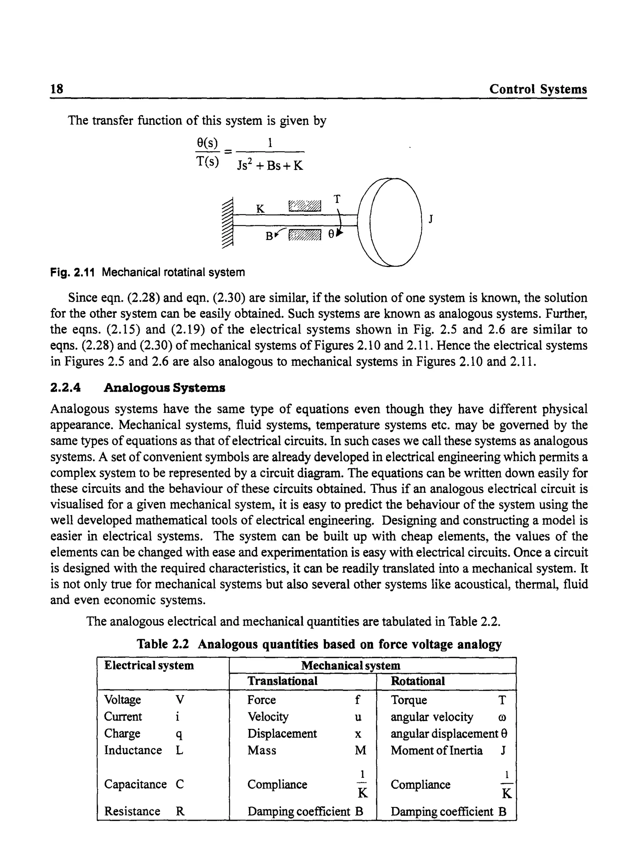
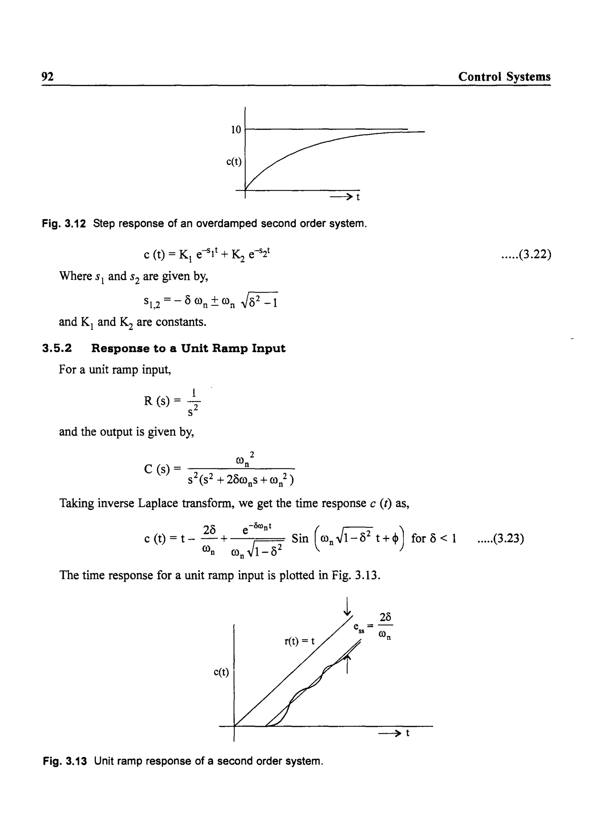
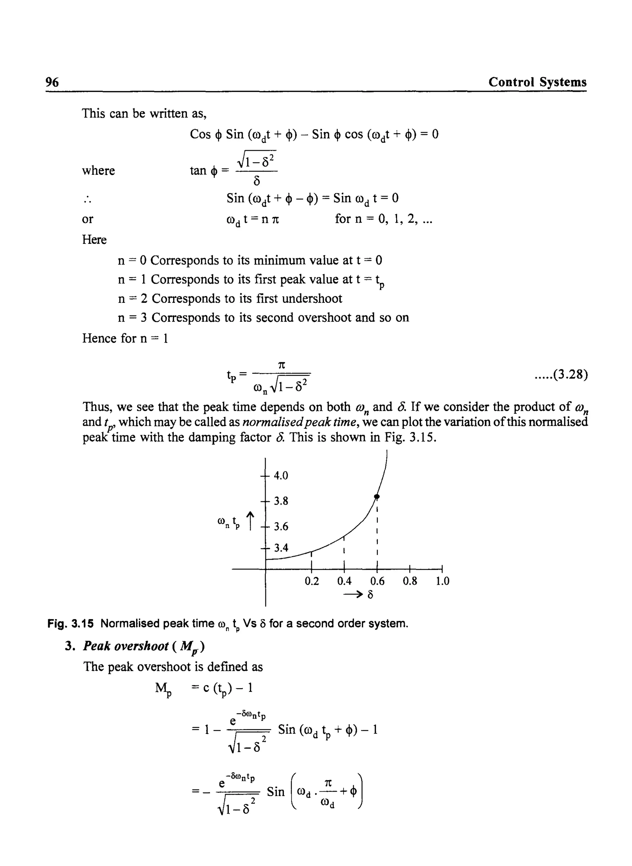
99. 90 Control Systems
Where OJd = OJn ~ is known as the damped natural frequency of the system. If 0 > 1, the
two roots sl' s2 are real and we have an over damped system. If 0 = 1, the system is known as a
critically damped system. The more common case of 0 < 1 is known as the under damped system.
If ron is held constant and 8 is changed from 0 to 00, the locus of the roots is shown in Fig. 3.9.
The magnitude ofs1 or s2 is OJn and is independent of8. Hence the locus is a semicircle with radius OJn
until 0= 1. At 0= 0, the roots are purely imaginary and are given by sl 2 = ± jOJn• For 0= 1, the roots
are purely real, negative and equal to - OJn. As oincreases beyond unity:the roots are real and negative
and one root approached the origin and the other approaches infinity as shown in Fig. 3.9.
1m s
8=0
s-plane
8>1 8=1
----~------~~.-~-----------Res
--(J)n
Fig. 3.9 Locus of the roots of the characteristic equation.
1
For a unit step input R(s) = - and eqn. 3.16 can be written as
s
co 2 1
C(s) = T(s). R(s) = 2 n 2 • -
S + 28cons + COn S
Splitting eqn. (3.17) in to partial fractions, assuming oto be less than 1, we have
C ( )
- Kl K2s +K3S - - +----=------=-------:-
S S2 + 28cons + con2
Evaluating K1, K2 and K3 by the usual procedure, we have,
1 s + 28conC (s) = - - --------7---
S (s + 8COn)2 + con2(1- ( 2)
.....(3.17)
s ~1-82 (S+8COn)2 + COn2(1_82
)
.....(3.18)
Taking inverse Laplae transform of eqn. (3.18), we have
c(t)= 1- e-'-',' [cosm,JI-6' t+ hsmm,~t] .....(3.19)

100. Time Response Analysis of Control Systems 91
Eqn. (3.19) can be put in a more convenient from as,
Where ffid = ffin ~
and .....(3.20)
This response is plotted in Fig. 3.10. The response is oscillatory and as t ~ 00, it approaches unity.
Fig. 3.10 Step response of an underdamped second order system.
If t5 = 1, the two roots of the characteristic equations are S I =. s2 = -OJn and the response is
given by
C(s)= (S+ffi
n
)2·;
and c (t) = 1 - e--<Ont
- t ffin e--<Ont
.....(3.21)
This is plotted in Fig. 3.11.
1.0 - - - - - - -
Fig.3.11 Response of a critically damped second order system.
As the damping is increased from a value less than unity, the oscillations decrease and when the
damping factor equals unity the oscillations just disappear. If t5is increaed beyond unity, the roots of
the characteristic equation are real and negative and hence, the response approaches unity in an
exponential way. This response is known as overdamped response and is shown in Fig. 3.12.

101. 92
l0r------------=====~--
c(t)
~t
Fig. 3.12 Step response of an overdamped second order system.
c (t) = Kl e-slt
+ ~ e-s
2t
Where sl and s2 are given by,
SI,2 =-8 ().)n±().)n ~
and Kl and K2 are constants.
3.5.2 Response to a Unit Ramp Input
For a unit ramp input,
1
R (s) = --
S2
and the output is given by,
().) 2
C (S) = n
S2(S2 +28rons+ron
2 )
Taking inverse Laplace transform, we get the time response c (t) as,
28 e-IiOOnt (c-;::;))c (t) = t - -- + Sin ron -Jl- 82
t + ~ for 8 < 1
ron ron ~l- 82
The time response for a unit ramp input is plotted in Fig. 3.13.
215
c(t)
Fig. 3.13 Unit ramp response of a second order system.
Control Systems
.....(3.22)
.....(3.23)

102. Time Response Analysis of Control Systems 93
The response reveals two aspects of the system.
I. The transient response is ofthe same form as that of a unit step response. No new information
is obtained regarding speed of response or oscillations in the system.
2. It has a steadystate error ess = 28 ,unlike the step response, where the steady state error was
wn
zero. Thus, no new information is gained by obtaining the transient response of the system for a
ramp input. The steadystate error could be easily calculated using final value theorem instead of
laboriously solving for the entire reponse. For the given system, the error E (s) is given by
E (s) = R (s) - C (s)
,., 2 2 21: 2 2
UJ
n _ S + uWns +Wn - Wn
S2 S2(S2 + 28wn
s +00/) - S2(S2 + 28wn
s +00/)
and from the final value theorem,
.....(3.24)
In a similar manner, the unit parabolic input does not yield any fresh information about the transient
response. The steadystate error can be obtained using final value theorem in this case also. For the
given system, for a unit acceleration input,
3.5.3
e = ao55
Time Domain Specifications of a Second Order System
The performance of a system is usually evaluated in terms ofthe following qualities.
I. How fast it is able to respond to the input,
2. How fast it is reaching the desired output,
.....(3.25)
3. What is the error between the desired output and the actual output, once the transients
die down and steady state is achieved,
4. Does it oscillate around the desired value,
and 5. Is the output continuously increasing with time or is it bounded.
The last aspect is concerned with the stability of the system and we would require the system to
be stable. This aspect will be considered later. The first four questions will be answered in terms of
time domain specifications of the system based on its response to a unit step input. These are the
specifications to be given for the design of a controller for a given system.
In section 3.5, we have obtained the response ofa type I second order system to a unit step input.
The step response of a typical underdamped second order system is plotted in Fig. 3.14.

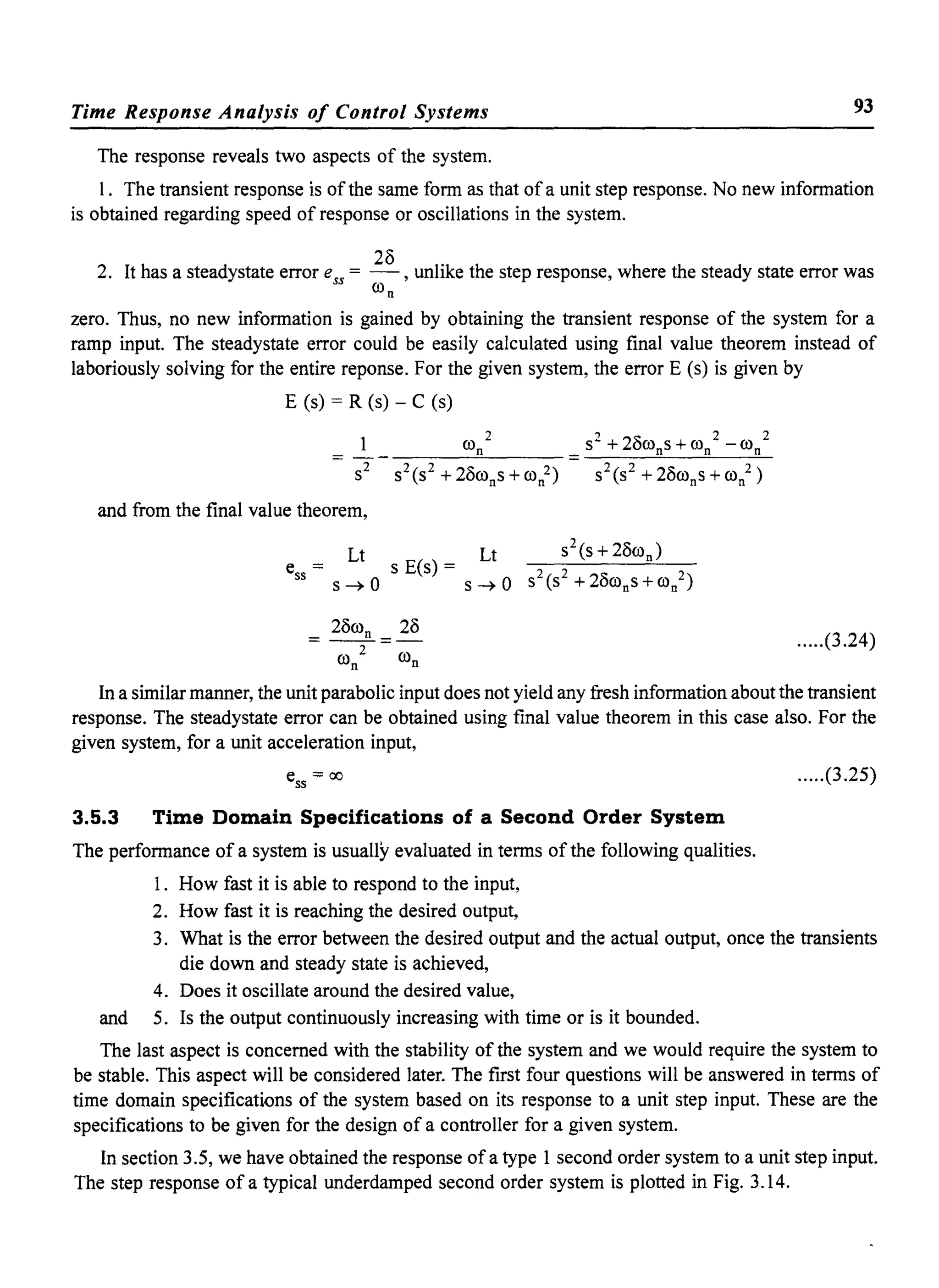
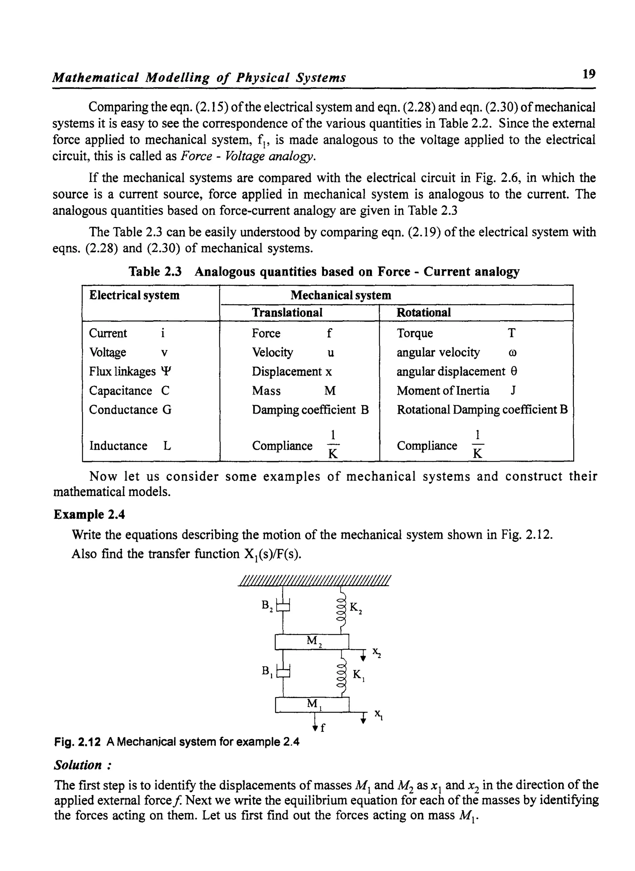
103. 94 Control Systems
It is observed that, for an underdamped system, there are two complex conjugate poles. Usually,
even if a system is of higher order, the two complex conjugate poles nearest to the j OJ - axis (called
dominant poles) are considered and the system is approximated by a second order system. Thus, in
designing any system, certain design specifications are given based on the typical underdamped step
response shown as Fig. 3.14.
2.0
c(t) t
1.0
0.5
"-
"
ts
Fig. 3.14 Time domain specifications of a second order system.
The design specifications are:
tolerance band
t--=-----=--=----
-== 1-=---
t.D
1. Delay time td: It is the time required for the response to reach 50% of the steady state value
for the first time
2. Rise time tr: It is the time required for the response to reach 100% of the steady state value
for under damped systems. However, for over damped systems, it is taken as the time required
for the response to rise from 10% to 90% of the steadystate value.
3. Peak time tp: It is the time required for the response to reach the maximum or Peak value of
the response.
4. Peak overshoot M : It is defined as the difference between the peak value ofthe response and
the steady state vafue. It is usually expressed in percent ofthe steady state value. Ifthe time for
the peak is tp' percent peak overshoot is given by,
c(tp) - c(oo)
Percent peak overshoot ~ = c(00) x 100. .....(3 .26)
For systems oftype 1 and higher, the steady state value c (00) is equal to unity, the same as the
input.
5. Settling time ts : It is the time required for the response to reach and remain within a specified
tolerance limits (usually ±2% or ±5%) around the steady state value.
6. Steady state error ess : It is the error betwen the desired output and the actual output as t ~ 00
or under steadystate conditions. The desired output is given by the reference input r (t) and
Lt
therefore, ess = [ret) - c(t)]
t~oo

104. Time Response Analysis of Control Systems 95
From the above specifications it can be easily seen that the time response of a system for a unit
step input is almost fixed once these specifications are given. But it is to be observed that all the above
specifications are not independent of each other and hence they have to be specified in such a way
that they are consistent with others.
Let us now obtain the expressions for some of the above design specifications in terms of the
damping factor 0 and natural frequency (On"
1. Rise time ( tT
)
If we consider an underdamped system, from the definition of the rise time, it is the time
required for the response to reach 100% of its steadystate value for the first time. Hence from
eqn. (3.20).
Or
e-&Dntr
Since r:--:::; cannot be equal to zero,
"1- 0
2
and
2. Peak time (tp )
Sin (rod tr + 4» = 0
rod tr + 4> = 1t
1t-4>
t = ----=====
r ron~
-I ~1-02
1t - tan
o .....(3.27)
At the peak time, tp, the response attains its maximum value and this can be obtained by
differentiating c (t) and equating it to zero. Thus,
-ocont
dc(t) oro --.'5 t • e
- - = n e (On SIll (rod t + 4» - -~==2= COS (rodt + 4». rod = 0
dt ~1-02 1-0
Simplifying we have,
o Sin (rodt + 4» - ~1- 02 cos (rodt + 4» = 0

105. 96
This can be written as,
where
or
Here
Cos ~ Sin (rodt + ~) - Sin ~ cos (rodt + ~) = 0
~1-o2
tan~= 0
for n = 0, 1, 2, ...
n = 0 Corresponds to its minimum value at t = 0
n = 1 Corresponds to its first peak value at t = tp
n = 2 Corresponds to its first undershoot
n = 3 Corresponds to its second overshoot and so on
Hence for n = 1
1t
t = -----;===
p ron~
Control Systems
.....(3.28)
Thus, we see that the peak time depends on both wn and 15. If we consider the product of wn
and tp' which may be called as normalisedpeak time, we can plot the variation ofthis normalised
peak time with the damping factor t5. This is shown in Fig. 3.15.
4.0
3.8
3.6
0.2 0.4 0.6 0.8 1.0
~o
Fig. 3.15 Normalised peak time ron tp Vs 0 for a second order system.
3. Peak overshoot ( MJT)
The peak overshoot is defmed as
~ = c (tp) - 1

106. Time Response Analysis of Control Systems
oronlt
e- ron~
Mp = ~ Sin ~ (": Sin (1t +~) = -Sin~)
-ltO
= e
k02
CSin~=~)
97
Hence, peak overshoot, expressed as a percentage of steady state value, is given by,
-ltO
M = 100 e
JI-02
%p .....(3.29)
It may be observed that peak overshoot My' is a function of the damping factor 0 only. Its
variation with damping factor is shown in rig. 3.16.
%Mp
100
80
60
40
20
0.2 0.4 0.6 0.8 l.0
-'0
Fig. 3.16 Percent overshoot Mp Vs 0 for a second order system.
4. Settling time ( ts )
The time varying term in the step response, c (t), consists of a product of two terms; namely,
-0 ront
an exponentially delaying term, h and a sinusoidal term, Sin (OJ; + rP). It is clear that
1-8
-oro t
the response is a decaying sinusoid, the envelop of which is given by b.Thus, the
1-8
response reaches and remains within a given band, around the steadystate value, when this
envelop crosses the tolerance band. Once this envelop reaches this value, there is no possibility
of subsequent oscillations to go beyond these tolerane limits. Thus for a 2% tolerance band,
e-0 ronts
r---2 = 0.02
"1-8
For low values of 0, (j « 1 and therefore e-O ronts ::::: 0.02
4
t---=4.
s - 8ro n
where .. is the time constant of the exponential term.
.....(3.30)

107. 98 Control Systems
Eqn. (3.30) shows that the settling time is a function ofboth 8and lVn. Since damping factor is an
important design specification, we would like to know the variation ofthe setting time with 8, with lVn
fixed. Or, in otherwords, we can define a normalised time lVis' and find the variation ofthis quantity
with respect to 8. The step response of a second order system is plotted in Fig. 3.17 for different
values of 8, taking normalised time lVi, on x-axis. The curves are magnified around the steady state
value for clarity.
c(t)
1.02
1.0
0.98
0.9
Fig. 3.17 C (t) plotted for different value of o.
0=0.76
The settling time monotonically decreases as the damping is decreased from a value greater than
one (over damped) to less than one (under damped). For 2% tolerance band, it decreases until the
first peak of the response reaches the tolerance limit of 1.02 as shown by the curve IV in Fig. 3.17.
Points A, B, C, and D marked on the graph give the values avs' for decreasing values of O. The peak
value of the response reaches 1.02 at a damping factor 8= 0.76. The settling time for this value of 8
is marked as point D on the curve. If 8 is decreased further, since the response crosses the upper
limit 1.02, the point E no longer represents the settling time. The settling time suddenly jumps to a
value given by the point F on the curve. Thus there is a discontinuity at 8 = 0.76. If 8 is decreased
further the setting time increases until the first undershoot touches the lower limit of 0.98. Similarly,
the third discontinuity occurs when the second peak touches the upper limit of 1.02 and so on. The
variation of lVis with 8 for a tolerance band of 2% is plotted in Fig. 3.18.
8
~6
liln ts i I~4 I: V
2 I 1 1
0.76 1
0.2 0.4 0.6 0.8 1.0
0.0
-70
Fig. 3.18 Variation of normalised settling time lilnt. Vs o.

108. Time Response Analysis of Control Systems 99
From Fig. 3.18 it is observed that the least settling time is obtained for a damping factor of
0= 0.76. Since settling time is a measure of how fast the system reaches a steady value, control
systems are usually designed with a damping factor of around 0.7. Sometimes. the systems are
designed to have even lesser damping factor because of the presence of certain nonlinearities which
tend to produce an error under steadystate conditions. To reduce this steadystate error, normally the
system gain K is increased, which in turn.decreases the damping (.: 8 = 2.J~T J.However, for
robotic control, the damping is made close to and slightly higher than unity. This is because the output
of a robotic system should reach the desired value as fast as possible, but it should never overshoot it.
S. Steady state error (ess)
For a type 1 system, considered for obtaining the design specifications of a second order control
system, the steady state error for a step input is obviously zero. Thus
Lt
ess = 1 - c(t) = 0
t~oo
The steady state error for a ramp input was obtained in eqn. (3.24) as ess = 28
ron
As the steadystate error, for various test signals, depends on the type of the system, it is dealt in
the next section in detail.
3.6 Steady State Errors
One of the important design specifications for a control system is the steadystate error. The steady
state output of any system should be as close to desired output as possible. If it deviates from this
desired output, the performance of the system is not satisfactory under steadystate conditions. The
steadystate error reflects the accuracy of the system. Among many reasons for these errors, the
most important ones are the type ofinput, the type ofthe system and the nonlinearities present in the
system. Since the actual input in a physical system is often a random signal, the steady state errors
are obtained for the standard test signals, namely, step, ramp and parbaolic signals.
3.6.1 Error Constants
Let us consider a feedback control system shown in Fig. 3.19.
R(s) C(s)
Fig. 3.19 Feedback 'Control System.

109. 100
The error signal E (s) is given by
E (s) = R (s) - H (s) C (s)
But C (s) = G (s) E (s)
From eqns. (3.31) and (3.32) we have
E (s) - R(s)
- 1+ G(s)H(s)
Applying fmal value theorem, we can get the steady state error ess as,
e
ss
= Lt s E(s) = Lt sR(s)
s ~ 0 s ~ 0 I+G(s)H(s)
Control Systems
.....(3.31)
.....(3.32)
.....(3.33)
Eqn. (3.33) shows that the steady state error is a function of the input R(s) and the open loop
transfer function G(s). Let us consider various standard test signals and obtain the steadystate error
for these inputs.
1. Unit step or position input.
1
For a unit step input, R (s) = -. Hence from eqn. (3.33)
s
Lt
1
s.-
s
s ~ 0 1+ G(s)H(s)
1
1+ Lt G(s) H(s)
s~
Let us define a useful term, position error constant Kp as,
~ ~ Lt G(s) H(s)
s~O
In terms of the position error constant, ess can be written as,
1
e = - -
ss I+Kp
2. Unit ramp or velocity input.
For unit velocity input, R(s) = ~ and hence,
s
1
Lt s.-
e = s
ss s~O I+G(s)H(s>
Lt
sG(s)H(s)
s~O
Lt 1
s ~ 0 s + sG(s)H(s)
.....(3.34)
.....(3.35)
.....(3.36)
.....(3.37)

110. Time Response Analysis of Control Systems
Again, defining the velocity error constant K.. as,
Lt
K.. = s G(s) H (s)
s~O
e = -
55 Kv
3. Unit parabolic or acceleration input.
1
For unit acceleration input R (s) = 3"" and hence
s
ess
Lt s
Lt
s
2
G(s)H(s)
s~O
Defining the acceleration error constant Ka as,
Lt
K = s2 G(s) H(s)
a s~O
1
e = -
55 Ka
For the special case of unity of feedback system, H (s)
are modified as,
Lt
~ = s~o G(s)
Lt
K.. = sG (s)
s~O
and
Lt 2
K = s G (S)
a S~O
101
.....(3.38)
.....(3.39)
Lt
.....(3.40)
.....(3.41)
.....(3.42)
= 1 and eqns. (3.35) (3.38) or (3.41)
.....(3.43)
.....(3.44)
.....(3.45)
In design specifications, instead of specifying the steady state error, it is a common practice to
specify the error constants which have a direct bearing on the steadystate error. As will be
seen later in this section, if the open loop transfer function is specified in time constant form,
as in eqn. (3.3), the error constant is equal to the gain of the open loop system.
3.6.2 Dependence of Steadystate Error on Type of the System
Let the loop transfer function G (s) H (s) or the open loop transfer function G (s) for a unity feedback
system, be giv·en is time constant form.
K(Tz1s + 1)(Tz2s + I) - - --
G(s) = r
S (Tp1s +1)(Tp2s +I) - - --
.....(3.46)

111. 102 Control Systems
As s ~ 0, the poles at the origin dominate the expression for G(s). We had defined the type of a
system, as the number of poles present at the origin. Hence the steady state error, which depends on
Lt Lt Lt .
G(s), s G(s) or s2 G(s), IS dependent on the type of the system. Let us therefore
s~O s~O s~o
obtain the steady state error for various standard test signals for type-O, type-I and type-2 systems.
1. Type -0 system
From eqn. (3.46) with r = 0, the error constants are given by
'"
Similarly
Lt
~ = CJ(s)
s~o
Lt
~ = s CJ(s)
s~o
K = Lt S2 CJ(s) = 0
a s~O
Lt
s~o
Lt
s~o
.....(3.47)
The steady state errors for unit step, velocity and acceleration inputs are respectively, from
eqns. (3.34), (3.37) and (3.40),
2. Type 1 system
1 1 ( . )e55
= - - = - - step mput
I+Kp I+K
eS5
= _1_ = 00 (velocity input)
Kv
1
e = - = 00 (acceleration input)
55 K
a
For type 1 system, r = 1 in eqn. (3.46) and
and
~ = Lt (}(s)
s~O
K
= Lt - = 00
s
Lt Lt K
~ = s CJ(s) = s. - = K
s~O s~O s
Lt Lt K
K = s CJ(s) = s2. - = 0
a s~O s~O S
The steady state error for unit step, unit velocity and unit acceleration inputs are respectively,
1 1
e = - - = - =0
S5 l+K 00
p
(position)

112. Time Response Analysis of Control Systems 103
1 1
e = - = - (velocity)
55 Ky K
and (acceleration)
3. Type 2-system
For a type - 2 system r = 2 in eqn. (3.46) and
K = Lt G(s)
-" s ~O
Lt K
-=00
s~O S2
Lt Lt sK
~ = s G(s) -=00
s~O s~O S2
Lt Lt s2K
and Ka = s2 G(s) -=K
s~o s~O S2
The steady state errors for the three test inputs are,
and
1 1
e = - - = - - = 0 (position)
5S I+Kp 1+00
1 1
e=-=-=O
ss Ky 00
1 1
ess = K= K
a
(velocity)
(acceleration)
Thus a type zero system has a fmite steady state error for a unit step input and is equal to
1 1
e =--=--
5S I+K I+Kp
.....(3.47)
Where K is the system gain in the time constant from. It is customary to specify the gain of a
type zero system by ~ rather than K.
Similarly, a type -1 system has a finite steady state error for a velocity input only and is given
by
1 1
eS5
= K = K .....(3.48)
y
Thus the gain of type -1 system in normally specified as ~.
A type -2 system has a finite steady state error only for acceleration input and is given by
1 1
ess = K =Ka
As before, the gain of type -2 system is specified as Ka rather than K.
.....(3.49)

113. 104 Control Systems
The steady state errors, for various standard inputs for type - 0, type - 1 and type - 2 are
summarized in Table. 3.1.
Table. 3.1 Steady state errors for various inputs and type of systems
Steadystate error ess
Standard input Type-O Type -1 Type - 2
Lt Lt Lt
~= G(s) ~ = s G(s) K = s2 G(s)
s~O s~O a s~ 0
1
Unit step - - 0 0
I+Kp
1
Unit velocity ao - 0
Kv
1
Unit acceleration ao ao -
Ka
If can be seen from Table. 3.1, as the type of the system and hence the number of integrations
increases, more and more steady state errors become zero. Hence it may appear that it is better to
design a system with more and more poles at the origin. But if the type of the system is higher than
2, the systems tend to be more unstable and the dynamic errors tend to be larger. The stability aspects
are considered in chapter 4.
3.6.3 Generalized Error Coefficients - Error Series
The main disadvantage of defining the.steadystate error in terms of error constants is that, only one
of the constants is finite and non zero for a particular system, where as the other constant's are either
zero or infmity. Ifany error constant is zero, the steady state error is infinity, but we do not have any
clue as to how the error is approaching infinity.
If the inputs are other than step, velocity or acceleration inputs, we can extend the concept of
error constants to include inputs which can be represented by a polynomial. Many functions which
are analytic can be represented by a polynomial in t. Let the error be given by,
R(s)
E(s)= I+G(s)
Eqn. (3.50) may be written as
Where
E (s) = Yes). R(s)
. 1
Y(s)- - -
1+ G(s)
.....(3.50)
.....(3.51)
.....(3.52)

114. Time Response Analysis of Control Systems
Using Convolution theorem eqn. (3:51) can be written as
t
e (t) = f Y (''C) r (t - .) d.
o
105
.....(3.53)
Assuming that r (t) has first n deriratives, r (t - r) can be expanded into a Taylor series,
, .2" .3",
r (t - .) = r (t) - • r (t) + 2! r (t) - 3! r (t) .....(3.54)
where the primes indicate time derivatives. Substituting eqn. (3.54) into eqn. (3.53), we have,
e (t) = J y (.) [r(t)-.r'(t)+~r"(t)-~r"'(t)----l d.
o 2! 3!
t , t " t .2
= r (t) f y (.) d • - r (t) f • y (.) d • + r (t) f -2' y (.) d • + ....
o 0 0 •
.....(3.55)
To obtain the steady state error, we take the limit t ~ ao on both sides of eqn. (3.55)
e = e (t) = r(t) fy(.)d. - r'(t) f-cy(.)d. + r" (t)-y(.)d......
Lt Lt [t t .2]ss t~ao t~ao 0 0 2!
.....(3.56)
Q() Q() Q() .2ess =rss (t) f y (.) d. - r'ss (t) f -cy (.) d. + rss" (t) f -2 y(.) d. + .....
o 0 0 !
.....(3.57)
Where the suffix ss denotes steady state part of the function. It may be further observed that the
integrals in eqn. (3.57) yield constant values. Hence eqn. (3.57) may be written as,
, C2 " C (n)
ess = Co rss (t) + C1 r ss (t) + -, r ss (t) + ... + ~ r S5 (t) +
2. n.
Where,
Q()
Co = f y(.) d.
o
Q()
C1 =- f .y (.) d.
o
Q()
Cn= (_I)n f ~ (.) d.
o
......(3.58)
.....(3.59)
.....(3.60)
.....(3.61)

115. 106 Control Systems
The coefficients Co' Cl' C2, .•. Cn' ... are defined as generalized error coefficients. Eqn. (3.58) is
known as generalised error series. It may be observed that the steady state error is obtained as a
function of time, in terms of generalised error coefficients, the steady state part of the input and its
derivatives. For a given transfer function G(s), the error coefficients can be easily evaluated as
shown in the following.
Let yet) = 1:1 Yes)
00
Yes) = J yet) e-s'r d.
o
Lt
yes)
s~o
00
J y ('t) d.
o
Co
Taking the derivative of eqn. (3.62) with respect to s,
We have,
dyes) = j y (.) (_.) e-st d •
ds 0
Now taking the limit of equation (3.64) as s ~ 0, we have,
Lt dyes) = j y (.) (_ 't) Lt e-5'r d 't
s~o ds 0 s~O
o
Similarly,
C = Lt d2
y(s)
2 s~O ds2
C = Lt d3
y(s)
3 s~O ds3
C = Lt dny(s)
n s ~ 0 dsn
.....(3.62)
.....(3.63) "
.....(3.64)
.....(3.65)
.....(3.66)
.....(3.67)
.....(3.68)
Thus the constants can be evaluated using eqns. (3.63), (3.65) and (3.66) and so on and the time
variation of the steadystate error can be obtained using eqn. (3.58).

116. Time Response Analysis of Control Systems 107
The advantages of error series can be summarized as,
1. It provides a simple way of obtaining the nature of steadystate response to almost any arbitrary
input.
2. We can obtain the complete steadystate response without actually solving the system differential
equation.
Example 3.1
The angular position 9c of a mass is controlled by a servo system through a reference signal 9r
. The
moment of intertia of moving parts referred to the load shaft, J, is 150 kgm2 and damping torque
coefficient referred to the load shaft, B, is 4.5 x 103 Nwm / rad / sec. The torque developed by the
motor at the load is 7.2 x 104 Nw-m per radian of error.
(a) Obtain the response of the system to a step input of 1 rad and determine the peak time, peak
overshoot and frequency oftransient oscillations. Also find the steadystate error for a constant
angular velocity of 1 revolution / minute.
(b) If a steady torque of 1000 Nwm is applied at the load shaft, determine the steadystate error.
Solution:
The block diagram of the system may be written as shown in Fig. 3.20.
Fig. 3.20 Block diagram of the given system
From the block diagram, the forward path transfer function G (s) is given by,
KTG(s) - -----'--
s(Js+ B)
For the given values of Kp J and B, we have
Thus
and
7.2xl04
G(s) = s(l50s + 4.5 x 103 )
16
s(0.333s +1)
Kv= 16
't = 0.333 sec.
1 1
= 2~Kv't = 2.J16 x 0.0333
= 0.6847

117. 108
(a)
Control Systems
= ~K.V - ~0.~~33
= 21.91 rad/sec
a(t)
e-ron! (~ _ f1=82i= 1- ~ Sin con "l-o- t+tan V~-o-)
Peak time,
= 1 - 1.372 e-15 t Sin (15.97 t + 46.80)
7t 7t
= co
n
JI-02 = COd
7t
= -- = 0.1967 sec
15.97
Peak over shoot, Mp
ltll
= 100 e- ~1-1l2
= 5.23%
Frequency of transient oscillations, cod = 15.97 rad/sec
. 27t
Steady state error 9R = - rad/sec
60
~= 16
27t
ess = 60 x16 = 6.54 x 10-3
rad
(b) When a load torque of 1000 Nwm is applied at the load shaft, using super position theorem,
the error is nothing but the response due to this load torque acting as a step input with
Fig. 3.21 Block diagram of the system with load torque applied
OR = O. The block diagram may be modified as shown in Fig. 3.21.
From Fig. 3.21, we have
1
Oc(s) = s(Js+B)
TL(s) 1+ Kr
s(Js+B)
1000
°c(s) = -s(-1-50-s-2 -+-4-.5-x-l-0-3 s-+-7-.-2-x-l0-4-)

118. Time Response Analysis of Control Systems
Using final value theorem,
Lt 1000
s~O s8c (s)= 7.2x104
= 0.01389 rad
= 0.796°
Example 3.2
The open loop transfer function of a unity feedback system is given by,
K
G(s)- - - -
s(,tS +1)
K, 't>0
109
With a given value of K, the peak overshoot was found to be 80%. It is proposed to reduce the
peak overshoot to 20% by decreasing the gain. Find the new value of K in terms of the old value.
Solution:
Let the gain be KI for a peak overshoot of 80%
1tIlJ
e-JHJ2 = 0.8
1t8 1
-====J= = In - = 0.223
Jl-8~ 0.8
1t2 81
2 = 0.2232 (1 - ( 2)
Solving for 81' we get
81 = 0.07
Let the new gain be Kz for a peak overshoot of 20%
Solving for 82,
82 = 0.456
1
But 8 = 2JK.
~ ~ ~.2JK" ~ t,82 2 KJ't KJ

119. 110 Control Systems
Example 3.3
Find the steadystate error for unit step, unit ramp and unit acceleration inputs for the following
systems.
1.
10
s(O.ls +1)(0.5s +1)
2.
1000(s + 1)
(s +10)(s + 50)
3.
Solution:
1.
(a)
10
G(s) - - - - - - -
s(O.ls +1)(0.5s +1)
Unit step input
Lt
~ = G (s) = CXl
s~O
1
ess = - - =0
l+Kp
(b) Unit ramp input
Lt
~ = s G(s)
s~O
Lt 10
------=10
s ~ 0 (O.1s +1)(0.5s +1)
1 1
ess = -=- = 0.1
Kv 10
(c) Unit acceleration input
Lt s2 G(s) = Lt lOs = 0
s ~ 0 s ~ 0 (O.ls +1)(0.5s +1)
1000
S2 (s + l)(s + 20)

120. Time Response Analysis of Control Systems
2.
3.
1000(s + 1)
G(s) - ------''------~
(s + 10)(s + 50)
The transfer function is given in pole zero fonn. Let us put this in time constant fonn.
G(s) = 500(0. Is + 1)(0.02s + 1)
1000(s+l) 2(s +1)
(O.ls + 1)(0.02s + 1)
Since this is a type zero system we can directly obtain
K" = 2, ~ = 0 Ka = 0
The steadystate errors are,
(a) Unit step input
1 1 1
e =--=--=-
551+Kp 1+2 3
(b) Unit ramp input
1 1
e =-=-=00
55 Ky 0
(c) Unit acceleration input
e =-=-=00
55 Ka 0
1000
G(s) - -::-----
- S2 (s + 1)(s + 20)
Expressing G (s) in time constant fonn,
1000 50
G(s) = 20S2 (s + 1)(0.05s + 1) = S2 (s + 1)(0.05s + 1)
The error constants for a type 2 system are
K" = 00 ~ = 00 Ka = 50
The steadystate errors for,
(a) a unit step input
1 1
e=--=-=O
55 I+K 00p
(b) a unit ramp input
1 1
e=-=-=O
55 Ky 00
(c) a unit acceleration input
1 1
e = -=- =0.02
55 Ka 50
111

121. 112 Control Systems
Example 3.4
The open loop transfer function of a servo system is given by,
G(s) = 10
s(0.2s + 1)
Evaluate the error series for the input,
Solution:
3t2
ret) = 1 + 2t + 2
10
G(s)- - - -
s(0.2s + 1)
1 s(0.2s + 1)
Y(s) = 1+ G(s) =-1-+--:1'-::0-- =-0.---'2S'-=2-+-
S
-+...:....1-0
s(0.2s + 1)
The generalised error coefficients are given by,
Lt
Co = s~O Yes)
C1
C1
Lt s(0.2s + 1)
--'-:----'-- = 0
s~O 0.2S2 +s+lO
Lt dyes)
s~O ds
Lt (0.2s2 + s + 10)(0.4s + 1) - s (0.2s + 1)(O.4s + 1)
s~O (0.2s2 + s + 10)2
Lt lO(O.4s + 1)
s~O (0.2s2 + s + 10)2
10
= - =0.1
102
C = Lt
2
s~O
d2
y(s)
ds2
Lt
s~O
(0.2s
2
+ s + 10)2(4) -1O(O.4s + 1)[2(0.2s2
+ s + 10)(0.4s + 1)1
(0.2s2
+ s + 10)4
400-10(20)
------:-'-----'- = 0.02
(10)4

122. Time Response Analysis of Control Systems
The input and its deriatives are,
3t2
r(t) = 1+ 2 t + -
2
6t
r' (t) = 2 + - = 2 + 3t
2
r" (t) = 3
r'" (t) = 0 = riv (t) = rV (t)
The error series is given by,
C
ess (t) = Co rss (t) + C, rss' (t) + 2~ rss" (t)
e (t) = 0 (1 + 2t + 3t2) + 0.1 (2 + 3t) + 0.02 (3)
ss 2 2
= 0.23 + O.3t
3.7 Design Specifications of a Control System
113
A second order control system is required to satisfy three main specifications, namely, peak overshoot
to a step input (Mp), settling time (ts) and steadystate accuracy. Peak overshoot is indicative of
damping (b) in the system and for a given damping settling time indicates the undamped natural
frequency of the system. The steadystate accuracy is specified by the steadystate error and error can
be made to lie within given limits by choosing an appropriate error constant Kp, Kvor Ka depending
on the type of the system. If any other specifications like rise time or delay time are also specified,
they must be specified consistent with the other specifications. Most control systems are designed to
be underdamped with a damping factor lying between 0.3 and 0.7. Let us examine the limitations in
choosing the parameters of a type one, second order system to satisfy all the design specifications.
The expressions for 0, ts and ess are given by,
1
0= -==
2~Kv't
4
t =--
sown
.....(3.69)
.....(3.70)
ess = K .....(3.71)
v
In a second order system, the only variables are Kv and T. Even if both of them are variable, we
can satisfy only two out of the three specifications namely, 0, ts and ess' Generally, we are given a
system for which a suitable controller has to be designed. This means that the system time constant
is fixed and the only variable available is the system gain Ky. By using a proportional controller, the
gain can be adjusted to suit the requirement of the steadystate accuracy. If Ky is adjusted for an
allowable limit on steadystate error, this value of Ky is usually large enough to make the system
damping considerably less, as given by eqn. (3.69). Thus the transient behaviours of the system is
not satisfactory. Hence suitable compensation schemes must be designed so that the dynamic response
improves. Some control schemes used in industry are discussed in the next section.

123. 114
3.7.1 Proportional Derivative Error Control (PD control)
A general block diagram of a system with a controller is given in Fig. 3.22.
Controller System or plant
R(s)
~f,-__E(_S_)~_~_G_c_(s_)_~_M~_(--'S_)~~~~~~_[0[]_G_(_S)_I-~~~~~--l~~C(_S)
Fig. 3.22 General block diagram of a system with controller and unity feed back
For a second order, Type 1 system,
K'
G(s) - y
s('ts + 1)
Control Systems
By choosing different configurations for the controller transfer function Gc (s) we get different
control schemes. The input to the controller is termed as error signal or most appropriately, actuating
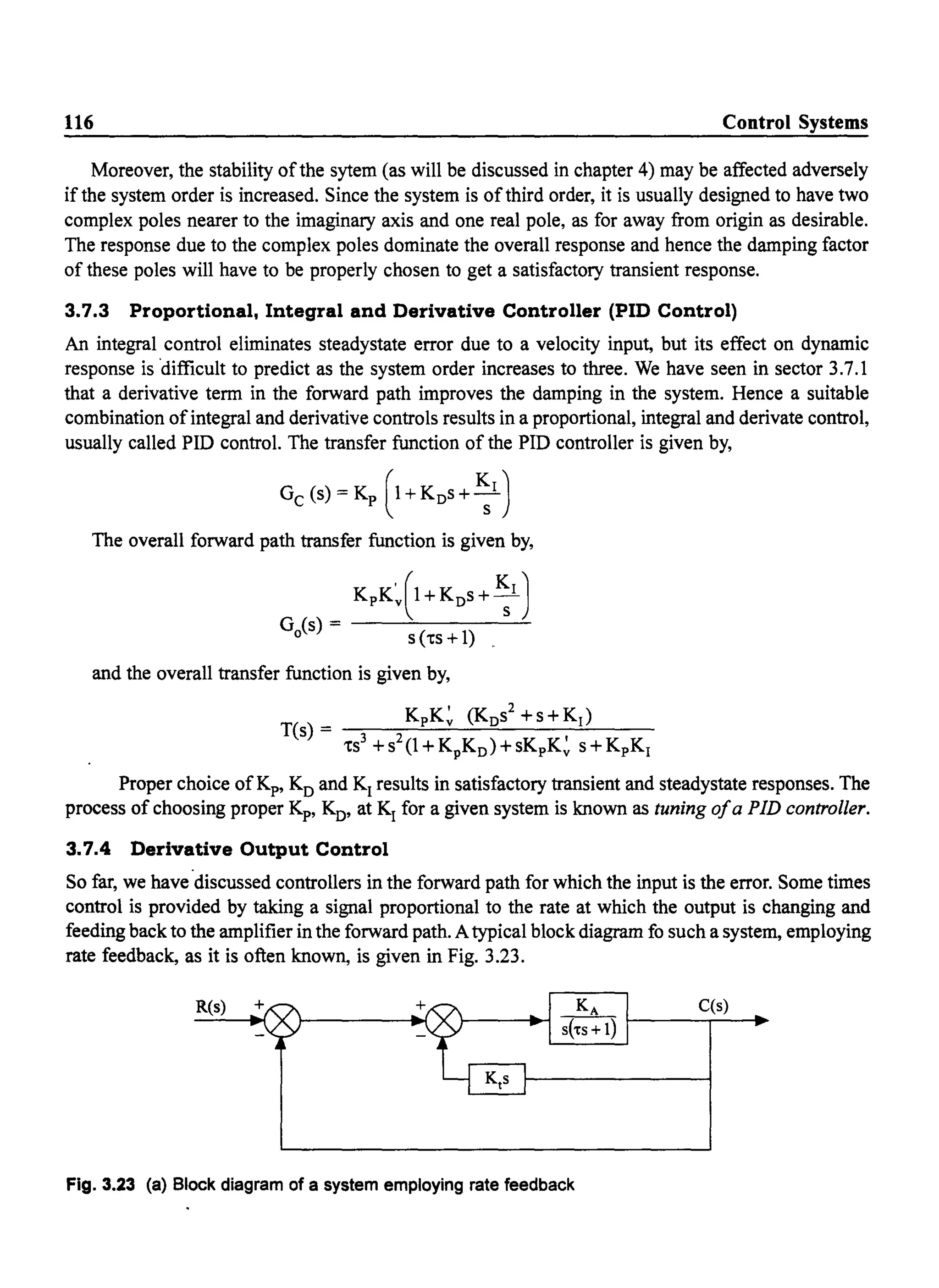
signal. The output ofthe controller is called as the manipulating variable, m(t) and is the signal given
as input to the system or plant. Thus, we have,
met) = Kp (e(t) + KD d:~t))
and M(s) = Kp (1 + KD s) E (s)
The open loop transfer function with PD controller is given by,
Go (s)= Gc (s) G (s)
Kp (1 + KDs)K~
s('ts + 1)
The closed loop transfer function of the system is given by,
Kp.K~ (K
D
s+1)
T(s) = __(:;-----''t'---_---.),---__
2 1+ KpKDK~ KpK~
s +s +---
't 't
If we define
K
-y(KD s+1)
T(s) = __.,:..'t------,.)--
2 (1+KyKD Kys +s +-
't 't
The damping and natural frequency of the system are given by,
, 1+ KyKD KD fK:-
8 = 2~Ky't = 8 + 2 ~~ .....(3.72)

124. Time Response Analysis of Control Systems 115
0) I = ~Kv = 0)
n t n
.....(3.73)
By a suitable choice ofthe proportional controller gain Kp (Amplifier gain), the steadystate error
requirements can be met. As seen earlier, such a choice of Kp usually results in a low value of
damping and hence this can be increased to a suitable value by of a proper choice of Ko' the gain of
the derivative term in the controller, as given by the eqn. (3.72). It can be observed from eqn. (3.73)
that the natural frequency is not altered for a given choice ofKp. Hence the settling time is automatically
reduced since (tJn is fixed and 8 for the compensated system has increased.
It may also be observed that, adding a derivative term in the controller introduces a zero in the
forward path transfer function and we have seen that the effect of this is to increase the damping in
the system.
3.7.2 Proportional Integral Controller (PI Control)
If the amplifier in the forward path is redesigned to include an integrator so that the output of the
controller is given by,
or
We have,
Where
and
and
m (t) = Kp (e(t) + K te(t)dt1
M (s) = Kp (1+ ~ ) E(s)
Go (s) = Gc (s) G (s)
1
T = -
1 K
Kp(s+K)K~
S2 (tS +1)
Kv(Ts + 1)
s2(ts+l)
.....(3.74)
.....(3.75)
.....(3.76)
From eqn. (3.75) we observe that the type of the system is changed from Type 1 to type 2 and
hence the steadystate error for a unit velocity input is reduced to zero. Hen& an integral controller is
usually preferred wherever the steadystate accuracy is important. But the dynamics of the system
can not be easily obtained, as the system order is increased from two to three, because of thl!
introduction of integral control.

125. 116 Control Systems
Moreover, the stability ofthe sytem (as will be discussed in chapter 4) may be affected adversely
if the system order is increased. Since the system is ofthird order, it is usually designed to have two
complex poles nearer to the imaginary axis and one real pole, as for away from origin as desirable.
The response due to the complex poles dominate the overall response and hence the damping factor
of these poles will have to be properly chosen to get a satisfactory transient response.
3.7.3 Proportional, Integral and Derivative Controller (PID Control)
An integral control eliminates steadystate error due to a velocity input, but its effect on dynamic
response is 'difficult to predict as the system order increases to three. We have seen in sector 3.7.1
that a derivative term in the forward path improves the damping in the system. Hence a suitable
combination ofintegral and derivative controls results in a proportional, integral and derivate control,
usually called PID control. The transfer function of the PID controller is given by,
Gc(s)=Kp (I+KoS+~r)
The overall forward path transfer function is given by,
KpK~(1+ Kos + ~r J
G (s) - ------''------'-
o s('rs+l) ,
and the overall transfer function is given by,
KpK~ (KOS2 + s + Kr)
T(s) = 3 2 I
'ts +s (I+KpKo)+sKpKy s+KpKr
Proper choice ofKp, KD and Kr results in satisfactory transient and steadystate responses. The
process of choosing proper Kp, KD, at Kr for a given system is known as tuning ofa PID controller.
3.7.4 Derivative Output Control
So far, we have'discussed controllers in the forward path for which the input is the error. Some times
control is provided by taking a signal proportional to the rate at which the output is changing and
feeding back to the amplifier in the forward path. Atypical block diagram fo such a system, employing
rate feedback, as it is often known, is given in Fig. 3.23.
R(s) + + C(s)
Fig. 3.23 (a) Block diagram of a system employing rate feedback

126. Time Response Analysis of Control Systems 117
The inner loop provides the desired rate feedback as its output is proportional to dc(t) . Simplifying
dt
the inner loop, we have,
E(s)
Fig. 3.23 (b) Simplified block diagram of Fig. 3.23 (a)
The forward path transfer function is given by,
KA
Where,
Thus the new damping factor is given by,
0'
.2~Kv''t' - 2 KA 't
l+Kt KA'l+Kt KA
_ l+KKA
- 2~KA't
= (1 + ~ KA) 0
The product, K'v 0' is given by,
K' 0' = KA =.!JKA
y 2~KA't 2 't
or KA = 4 (K'yO'Y 't
C(s)
.....(3.77)
.....(3.78)
.....(3.79)
.....(3.80)
.....(3.81)
.....(3.82)
.....(3.83)

127. 118 Control Systems
If the values of K 'v and () I are specified, the amplifier gain (KA) can be adjusted to get a suitable
value using eqn. (3.82). For this vlaue of KA' the rate feedback constant ~ is given by, using
eqn.3.78,
If rate feedback is not present,
~=KA
1
and () = --;==
2~KA't
.....(3.84)
.....(3.85)
With rate feedback, if same velocity error constant is specified, comparing eqn. (3.78) with eqn.
(3.85), we see that the amplifier gain, KA has to be more. Thus aJn I given by eqn. (3.82) will be
more. Hence the derivative output compensation increases both damping factor and natural frequency,
thereby reducing the settilng time.
3.5 Example
Consider the position control system shown in Fig. 3.24 (a). Draw the block diagram of the system.
The particulars of the system are the following.
Total Moment oflnertia referred to motor shaft, J = 4 x 10-3 kgm2.
Total friction coefficient referred to motor shaft, f = 2 x 10-3 Nwm[rad[sec
Motor
L...-_ _ _ _ _ _r="'FLK_A~---.:RJ:::;:a::::..-
I
A.;r }- _ 1-___T"hogen"":;:.t....:_.
K
Fig. 3.24 (a) Schematic of a position control system.
Motor to load Gear ratio, n = 8L
= _1_
8M 50
eLoad to potentiometer gear ratio, eL = 1
c

128. Time Response Analysis of Control Systems
Motor torque constant,
Tachogenerator constant,
Sensitivity of error detector,
Amplifier gain,
KT = 2 Nw-m Iamp
~ = 0.2V Irad Isec
Kp = 0.5V Irad.
KAAmpsN. (variable)
119
(a) With switch K open, obtain the vlaue of KA for a steadystate error of 0.02 for unit ramp
input. Calculate the values ofdamping factor, natural frequency, peak overshoot and settling
time.
(b) With switch K open, the amplifier is modified to include a derivative term, so that the armature
current ia (t) is given by
ia (t) = KA (e(t) + KD d~~t))
Find the vlaues ofKA and Ko to give a steadystate error within 0.02 for a unit ramp input and
damping factor of 0.6. Find the natural frequency and settling time in this case.
(c) With switch K closed and with proportional control only, find the portion of tachogenerator
voltage to be fedback, b, to get a peak overshort of 20%. Steadystate error should be less
than 0.02 for a unit ramp input. Find the settling time and natural frequency.
Solution: The block diagram of the system is given in Fig. 3.24 (b).
Fig. 3.24 (b) Block diagram of the position control system of Fig. 3.24 (a).
With switch K open,
0.5 x 2KA
50 . s(4xlO-3s+2xlO-3 )
50x2xl0-3
s(2s+1)
s(2s + 1)
10KA
s(2s +1)

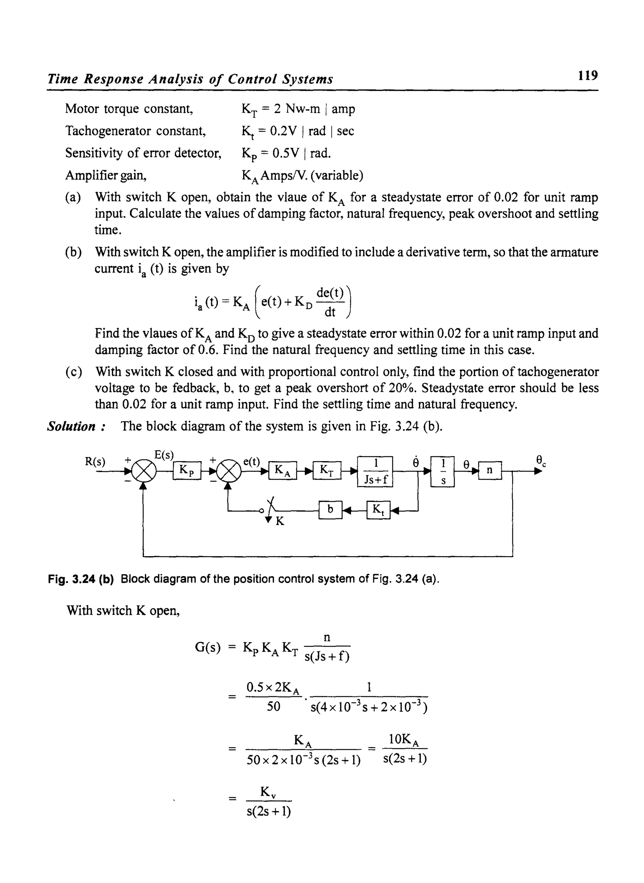
129. 120
Now
damping factor,
Natural frequency,
Peak overshoot,
Settling time,
ess = 0.02
1 1
KA = 10xO.02 = S
K.. = 10 KA = SO
1 1 1
(5 = = =- O.OS
2~Kv't 2.JSO x 2 20
ro = fK: = {SO
n ~-;- f"2
= S.O rad/sec.
118
M = e-~1-82 = 8S.4S%p
4 4
t = - = x S = 16 sec
S (5ron O.OS x S
Control Systems
Thus, it is seen that, using proportional control only (Adjusting the amplifier gain KA) the steadystate
error is satisfied, but the damping is poor, resulting in highly oscillatory system. The settling time is
also very high.
(b) With the amplifier modified to include a derivative term,
ia(t) = KA [e(t) + Ko d~~t)]
The forward path transfer function becomes,
KpKA(1+Kos)KTn 0.SxKA(1+Kos)2 10KA(1+Kos)
G(s) = s(Js + f) =2 x 10-3 x SOs(2s + 1) = s(2s + 1)
To satisfy steadystate error requirements, KA is again chosen as S. The damping factor is
given by,
1+ SOKo
0.6 = 2.JSO x 2
From which we get,
Ko= 0.22

130. Time Response Analysis of Control Systems 121
~v ~oco = - = - = 5 rad/sec
n 't 2
4
ts = 0.6 x 5 = 1.333 sec
The derivative control increases the damping and also reduces the setlling time. The natural
frequency is unaltered.
(c) With switch K closed and with only proportional control, we have,
G(s) = K:.n [JS + f ~~~~TKtb1
0.5 [ 2KA 1= 50s 4xlO-3
s+2xlO-3
+2xO.2xKAb
The closed loop transfer function is given by,
KA
T(s) = --=-~---'-'---:----
0.2S2 +(0.1+20KAb)s+KA
The steadystate error, ess = 0.02
1
~= - =50
0.02
The peak over shoot,
7t6
Mp = e-)1-6
2
= 0.2
(5 = 0.456
From the expression for G (s), we have,
Lt
~ = s~ 0 s G(s)
KA KA
~ = 50(2 x 10-3 +O.4KAb) = 0.1 +20KAb
From the expression for T (s), we have
0.1 + 20KAb
(5 = 0.2

131. 122 Control Systems
Taking the product of ~ and 0, we have
KA 0.1+20KAb
~o = x--===-
0.1 + 20KAb 2~0.2KA
KA
2~0.2KA
But ~ = 50 and 0 = 0.456
x 2 _ K~
(50 0.456) - 4xO.2KA
KA = 4 x 0.2 (50 x 0.456)2 = 415.872
We notice that the value of KA is much larger, compared to KA in part (a). Substituting the
value of KA in the expression for ~, we have,
415.872
50=-------
0.1 + 20x 415.872x b
b can be calculated as,
b = 0.001
{K; ~415.872
The natural frequency ron = V02 = 0.2 = 45.6 rad/sec
Comparing ron in part (a), we see that the natural frequency has increased. Thus the setlling
time is redued to a value give by,
4 4
t = -= = 0.1924 sec.
s oron 0.456 x 45.6
This problem clearly illustrates the effects of P, P D and derivative output controls.
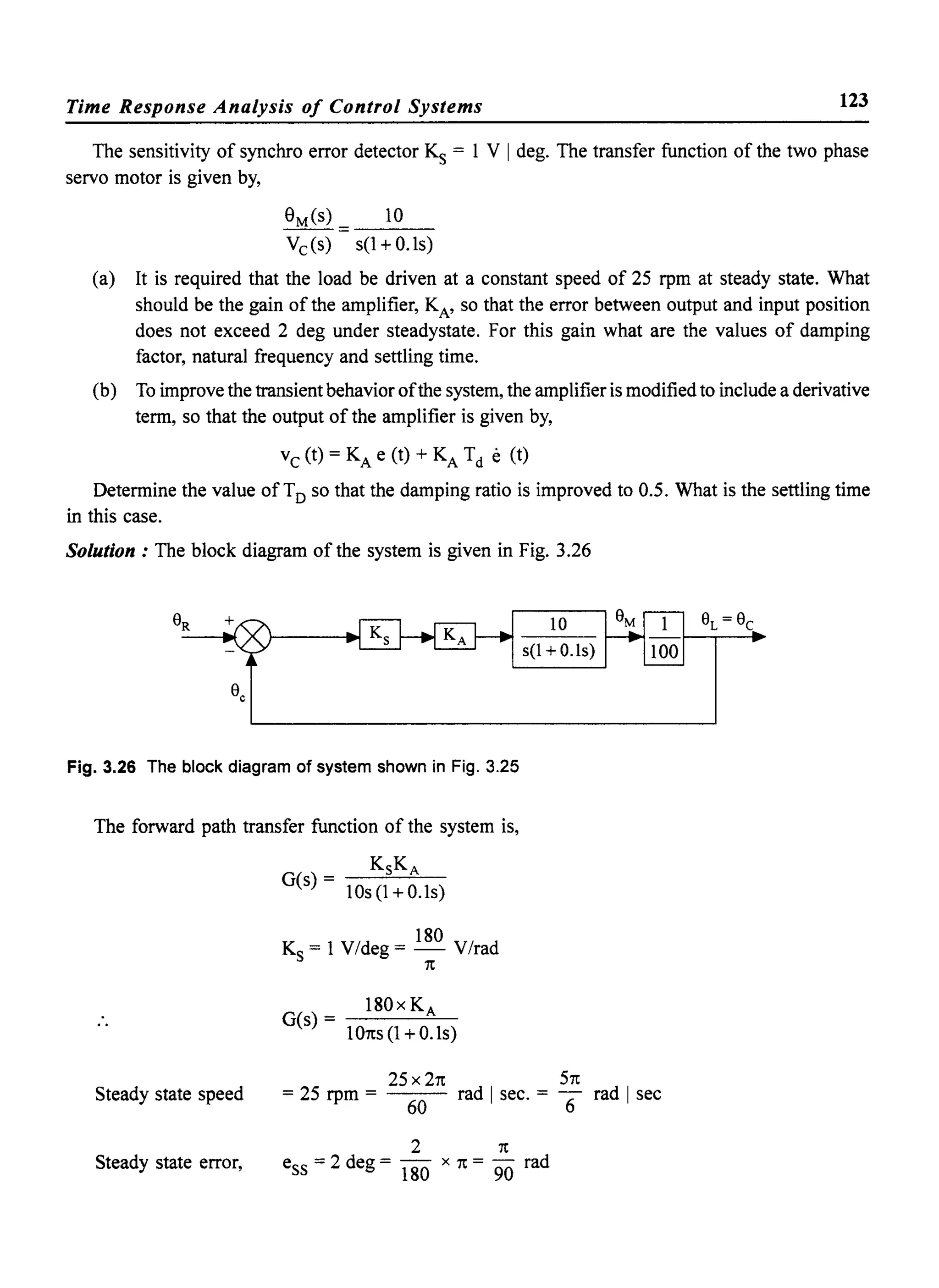
Example 3.6
Consider the control system shown in Fig. 3.25.
Synchro
• Ks
Fig. 3.25 Schematic of a control system for Ex. 3.6
Amplifier
gainKA
ac 8L = J.-
~ 8M 100
G7{]
servo
motor
9L
-=1
9c

132. Time Response Analysis of Control Systems 123
The sensitivity of synchro error detector Ks = 1 V I deg. The transfer function of the two phase
servo motor is given by,
aMeS) = 10
Vc(s) s(1+0.1s)
(a) It is required that the load be driven at a constant speed of 25 rpm at steady state. What
should be the gain of the amplifier, KA' so that the error between output and input position
does not exceed 2 deg under steadystate. For this gain what are the values of damping
factor, natural frequency and settling time.
(b) To improve the transient behavior ofthe system, the amplifier is modified to include a derivative
term, so that the output of the amplifier is given by,
Vc (t) = KA e (t) + KA Td e (t)
Determine the value of TD so that the damping ratio is improved to 0.5. What is the settling time
in this case.
Solution: The block diagram of the system is given in Fig. 3.26
Fig. 3.26 The block diagram of system shown in Fig. 3.25
The forward path transfer function of the system is,
KsKA
G(s) - -~-'-'--
10s(1+0.1s)
180
Ks = 1 V/deg = - V/rad
1t
180 x K A
G(s) = -----=-~
101ts(1+0.1s)
10
s(1 +O.1s)
Steady state speed
25 X 21t 51t
= 25 rpm = rad I sec. = -6 rad I sec
60
2 1t
Steady state error, ess = 2 deg = 180 x 1t = 90 rad

133. 124
For the given system,
~=
ess =
But ess
Lt
s-+O
Lt
s-+O
ISKA
1t
51t
--=
6Kv
1t
90
51t2
s G(s)
sxlS0x KA
1ts(1 + 0.ls)10
51t X 1t
6 x lSKA
1t
.. =-
10SKA 90
From which, we get, KA = 13.1
75
G (s) - - - -
c s(1+0.1s)
T(s)
= Sc(s) = 75
SR(S) 0.ls2 +s+75
750
s2+10s+750
con = .J750 = 27.39
C3 1 1 = 0.IS26
2~Kv't 2.J75 x 0.1
4 4
t = - = = O.S sec
s C3con 0.IS26x27.39
(b) When the amplifier is modified as,
Vc (t) = KAe (t) + KA TD e(t)
The open loop transfer function becomes,
KsKA (1 + TDs)
G(s) = 10s(0.ls+l)
Control Systems

134. Time Response Analysis of Control Systems
Se(s) KsKA(1+Tos)
T(s) = SR (s) = S2 + (10 + KsKATo)s + KsKA
180 x 13.1(1 + Tos)
---,--------~--~~------ x -
(
180 ) 180 7t
S2 + 10+--;-xI3.1To s+--;-xI3.l
S2 +(10+750To )s+750
ron = .J750 = 27.39
28 ron = 10 + 750 TD
T = 28ron -10 =2 x 0.5 x 27.39 -10 = 0.0232
D 750 750
4 4
t5 = 8ro
n
=0.5 x 27.39 =0.292 see
125
Thus, we see that, by including a derivative tenn in the amplifier, the transient perofrmance is improved.
It may also be noted that ~ is not changed and hence the steady state error remains the same.
Problems
3.1 Draw the schematic of the position control system described below.
Two potentiometers are used as error detector with SR driving the reference shaft and the
load shaft driving the secind potentiometer shaft. The error signal is amplified and drives a
d c. Servomotor armature. Field current of the motor is kept constant. The motor drives the
load through a gear.
Draw the block diagram of the system and obtain the closed loop transfer function. Find the
natural frequency, damping factor, peak time, peak overshoot and settling time for a unit step
input, when the amplifier gain KA = 1500. The parameters of the system are as follows:
Potentiometer sensitivity Kp = 1VIrad
Resistance of the annature
Equivalent Moment of Inertia at motor shaft
Equivalent friction at the motor shaft
Motor torque constant
Gear ratio
Motor back e.m.f constant
Ra = 20
J = 5 x 10-3 kg-m2
B = 1 x 10-3 NW/rad/sec
KT = 1.5 Nro mlA
1
n= --
10
Kb = 1.5 VIrad/sec

135. 126 Control Systems
3.2 A position control system is shown in Fig. P 3.2
<"E---,--- - - - - - - -
R ~Ira
Fig. P3.2
24
Sensitivity of the potentiometer error detection Kp = - VIrad
1t
Amplifier gain
Armature resistance
Motor back e.m.f constant
Motor torque constant
Moment of Inertia of motor referred to motor shaft
Moment of Inertia of load referred to the output shaft
Friction coefficient of the load referred to the output shaft
N . 1
_1=_
N2 10
Gear ratio
KAVN
Ra = 0.2 n
Kb = 5.5 x 10-2 V/rad/sec
KT = 6 x 10-5 N-mlA
1m = 10-5 Kg m2
1L = 4.4 x 10-3 Kgm2
B = 4 x 10-2 Nmlrad/secv
(i) Ifthe amplifier gain is 10VN obtain the transfer function of the system C(s) = 8L (s) .
R(s) 8R (s)
Find the peak overshoot, peak time, and settling time ofthe system for a unit step input.
(ii) What values ofKA will improve the damping factor to 0.707
(iii) What value of KA will give the frequency of oscillations of9.23 rad/sec to a step input.
3.3 The open loop transfer function of a unity feed back control system is given by,
K
G(s)- - - -
seTs +1)
If the maximum response is obtained at t = 4 sec and the maximum value is 1.26, find the
values if K and T.

136. Time Response Analysis of Control.Systems 127
3.4 A unity feedback system has the plant transfer function
C(s) 10
O(s)- - - - - -
1 -M(s)-s(s+2)
A Proportional derivative control is employed to control the dynamics of the system. The
controller characteristics are given by,
de(t)
met) = e(t) + Ko dt
where e(t) is the error.
Determine
(i) The damping factor and undamped natural frequency when Ko= 0
(li) The value of Ko so that the damping factor is increased to 0.6.
3.5 Consider the system shown in Fig. P 3.5.
Fig. P3.5
(i) With switch K open, determine the damping factor and the natural frequency of the
system. If a unit ramp input is applied to the system, find the steady state output. Take
KA =5
(ii) The damping factor is to be increases to 0.7 by includinga derivative output compensation.
Find the value of~ to achieve this. Find the value of undamped natural frequency and
the steady state error due to a unit ramp input.
(iii) It is possible to maintain the same steady state error for a unit ramp input as in part (i)
by choosing proper values of KA and ~. Find these values.
3.6 In the system shown in Fig. P 3.6 find the values ofK and a so that the peak overshoot for
a step input is 25% and peak time is 2 sec.
C(s)
Fig. P3.6

137. 128 Control Systems
3.7 Determine the values of K and a such that the damping factor is 0.6 and a settling time of
1.67sec.
Fig. P3.7
Also find the step response of the system.
3.8 Find the steadystate errors for unit step, unit velocity and unit acceleration inputs for the
folloWing systems.
15
(i)
s(s + 1)(s + 5)
100
(iii) s2(0.ls + 1)(.Ols + 1)
(ii)
(iv)
10(0.ls+l)
(0.02s + 1)(0.2s + 1)
(s+2)(s+5)
s(0.2s +1)(0.6s + 1)
3.9 In the system shown in Fig P 3.7 fmd the value of K and a such that the damping factor of
the system is 0.6 and the steady state error due to a unit ramp input is 0.25.
3.10 For the unity feedback system with,
10
G(s) = - -
s+1O
Find the error series for the input,
3t2
vet) = 1 + 2t + 2
3.11 Find the steadystate error as a function of time for the unity feedback system,
100
, G(s) = s(l + O.ls)
for the following inputs.
t
2
(a) r (t) = 2" u(t)
-djl-
(b)
t
2
r (t) = 1 + 2t + -.
2

138. 4 Stability of Systems
4.1 Introduction
It is usually not desirable that a small change in the input, initial condition, or parameters of the
system produces a very large change in the response of the system. If the response increases
indefinitely with time the system is said to be unstable. Stability is an important property that a
system is required to possess. It is not only essential to design a system to obtain the desired
response, it is also necessary to design a system which is stable. Suppose we have a control system
which is designed to drive a load at a desired speed. For some reason ifthere is a small change in the
load on the motor, the motor speed should not increase indefinitely.
In general there are two concepts ofstability. The first one is known as a Bounded Input Bounded
Output stability (BIBO). According to this concept, if a bounded input is given to the system, the
output should be bounded. The second one is defined with no input to its system. If an initial
condition is applied to the system, the system should return to its eqUilibrium condition, which is
usually the origin. For linear time invariant systems the two concepts are equivalent. For non linear
systems, the determination ofstability is more complicated. Even ifa system is found to be stable for
a certain bounded input it may not be staple for another bounded input. Ifa nonlinear system is found
to be stable for certain initial condition, it may not be stable when a bounded input is given. Usually
nonlinear system stability is studied for autonomous systems i.e., systems without input. In contrast
to this, for a linear, time invariant system, there are simple criteria for determining the stability. In this
chapter, we will deal with an algebraic criterion for determining the stability of linear, time invariant
systems.

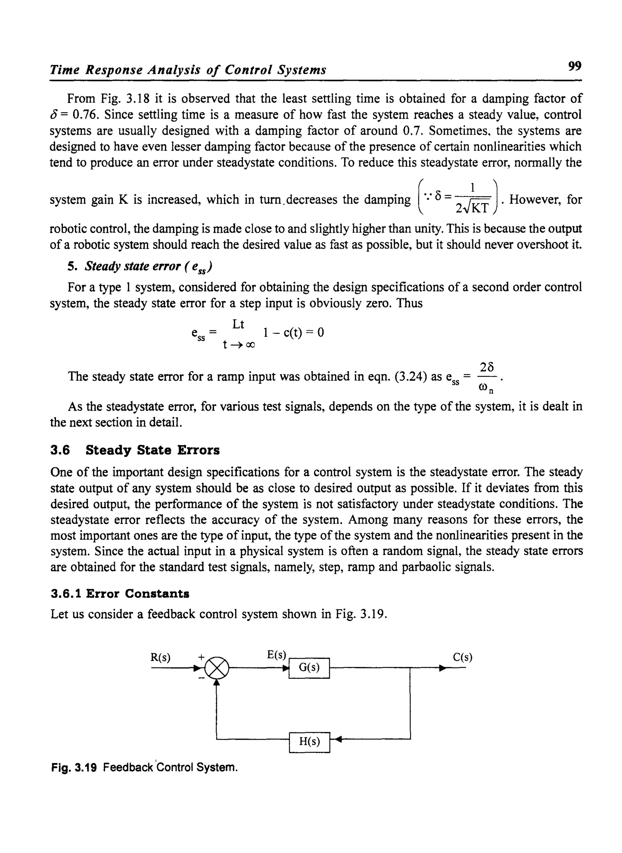
139. 130 Control Systems
4.2 Stability Preliminaries
The two concepts of stability are equivalent for linear time invariant systems. To see this, let us
consider the output of a linear, time invariant system, given by,
t
c(t) = f he-t) ret - .)d. .....(4.1)
o
where h(t) is the impulse response of the system,
and r(t) is the input to the system.
We know that [
C(S)]h(t) = l';-1[T(s)] = l';-I -
R(s)
and
b m b m-l boS + 1S +... +
T(s) = n n-l m
aos +a1s +...an
.....(4.2)
If the input is bounded, i.e., Ir(t)1 ~ Rl' we have from eqn. (4.1).
Ic(t)1 = [th (') ret - 't) d't[
t
~ f Ih('t)llr(t - .)1d.
o
t
~RI if Ih('t)ld't .....(4.3)
o
For a stable system, bounded input should produce bounded output. Hence from eqn. (4.3).
t
Ic(t)1 = RI I Ih('t)ld't ~ ~ .....(4.4)
o
t
Thus the system is Bmo stable, if I Ih('t)1 d't is finite or h(t) is absolutely integrable. If Ih (t)1 is
o
plotted with respect to time, this condition means that the area bounded by this curve and time axis
must be finite between the limits t = 0 and t = 00. Thus the stability ofthe system can be ascertained
from the impulse response or the natural response of the system which is independent of the input.
t
If I Ih('t)1 d't is bounded the response for any initial condition will also be bounded and the system will
o
return to its equilibrium condition.
Since the nature of impulse response '1(t) depends on the location of poles of T(s), the transfer
function T(s) is given by eqn. (4.2) and can be written as,
N(s)
T(s) = D(s) .....(4.5)

140. Stability of Systems 131
D(s) = 0 is known as the characteristic equation ofthe system and the poles ofTCs) are the roots
of D(s) = O. The roots of D(s) may be classified as :
(i) Real roots at s = cr
K
The transfer function T(s) contains terms like - - which give rise to terms like Keat in the
s-cr
impulse response. If cr is positive, the exponential term increases indefinitely with time and
h(t) is unbounded. If cr is negative, the response h(t) decreases with time and h(t) ~ 0 as
t ~ 00. The area under the curve of h(t) is bounded.
If real roots have multiplicity m, T(s) contains terms of the form,
Kr
(
l)i i = 1, 2, .....m
s -cr
which on inversion, gives rise to terms of the form Ai t1
-
1 eat, i = 1, 2, .....m
If cr is positive, these terms make h(t) unbounded. On the other hand if cr is negative, the
t
response dies down as t ~ 00 and Jlh(t)1 dt is bounded.
o
(..) C I ' . I tho ( ) . lik As + B11 omp ex conjugate roots at s = cr +Jco. n IS case T s contams terms e 2 2
(s - cr) + co
therefore, h(t) contains terms like Keat Sin (cot + ~)
and
Ifcr is positive i.e., ifthe real part ofthe root is positive, the amplitude ofsinusoidal oscillations
increases indefinitely and h(t) will be unbounded. If cr is negative h(t) will have oscillations
whose amplitudes tend to zero as t ~ 00 and thus, h(t) will be bounded.
If the complex conjugate roots are repeated with multiplicity m at s = cr + jco,
T(s) will contain terms like ~ Ai
S
+B1 J i = 1, 2, .........m.
(s - cr)2 +co2 I
which yields, on inversion,
C1tl-1Keat Sin (cot + ~.), i = 1,2, .....m
In this case also, if the real part ofthe complex root a is positive, the response is unbounded
and if it is negative, the response is bounded.
(iii) Roots at origin.
T(s) will have a term K , which gives rise to a constant term Ku(t), as the response. In this
s
co
case, although h(t) = Ku(t) is bounded, J Ih(t)1 dt is not bounded. If repeated roots at origin are
o
present in T(s), it will have terms like,
Kli
SI
i = 1,2, ..... m
which give rise to terms in the impulse response h(t), of the form,
C1tl- 1 fori=1,2, .... m
which clearly results in unbounded h(t).

141. 132 Control Systems
(iv) Purely imaginary roots at s = jOJ
As+B
Roots on imaginary axis will contribute terms like in T(s) and their inversion yields
S2 + ro2
terms of the form,
C Sin (rot + ~)
00
which have constant amplitude. In this case also even though h(t) is bounded f Ih(t)I dt is
o
not bounded.
If the imaginary roots are repeated, they yield terms like ~iS +~i. for i = 1,2, ....m in h (t).
(Si + ro y
These terms clearly make h(t) unbounded as t ~ 00.
To summarise, if the roots are negative, or have negative real parts if they are complex, the
00
impulse response h(t) is bounded and flh(t)1 dt is also bounded. The system will be BIBO
o
stable for these roots occuring in the left half of s-plane even ifthey are repeated. If the roots
are positive, or they have positive real parts if complex, the response is unbounded and hence
the system is unstable. The response is bounded ifthe roots are purely imaginary but simple. The
system is classified as marginally or limitedly stable, since the response will be oscillatory with
constant amplitude. The location of the roots and corresponding responses are given in
Fig. 4.1. The response is indicated near the corresponding root.
L
x x x
Fig. 4.1 Location of roots of characteristic equation and corresponding responses.

142. Stability of Systems 133
Based on the above observations regarding location of rOots of the characteristic equation and
stability ofthe system, the s-plane can be divided into two regions. The left side of imaginary axis is
the stable region and if roots of characteristic equation occur in this half of s-plane, the system is
stable. The roots may be simple or may occur with any multiplicity. On the other hand, even ifsimple
roots occur in the right half of s-plane, the system is unstable. If simple roots occur on the ja>-axis,
which is the boundary for these two regions, the system is said to be marginally or limitedly stable.
Ifroots onja>-axis are repeated, the system is unstable. The stable and unstable regions ofs-plane are
shown in Fig. 4.2.
jro
s-plane
Stable Unstable
Fig. 4.2 Demarcation of stable and unstable regions of s-plane.
Hence, determination of stability of a linear time invariant system boils down to determining
whether any roots of the characteristic equation or poles of transfer function lie in the right half of
s-plane. One obvious method of determining stability of a system is to find all the roots of
D(s) = aa sn + al
sn - 1 + ..... + an'
For a polynomial of degree n > 2, it is difficult to find the roots analytically. Numerical methods
for root determination for higher order polynomials is quite cumbersome. Hence, algebraic criteria
are developed to find out ifany roots lie in the right halfofs-plane. The actual location ofthe roots is
unimportant.
4.3 Necessary Conditions for Stability
In section 4.2 we have seen that the system will be stable ifthe roots ofthe characteristic equation lie
in the left half of s-plane. The factors of the characteristic polynomial D(s) can have terms like
(s + 0), (s + O"k)2 + rof
where 0"1 are positive and real. Thus
D(s) = aosn + al
sn - 1 + ..... +an .....(4.4)
= aoIT (s + 0"1) IT {(s + O"k)2 + rof} .....(4.5)
Since 0"1 and O"k are all positive and real the product in eqn. (4.5) results in all positive and real
coefficients in the polynomial of s. Thus if the system is stable all the coefficients, ai' must be
positive and real.
Further, since there are no negative terms involved in the product of eqn. (4.5), no cancellations
can occur and hence no coefficient can be zero. Thus none ofthe powers ofs in between the highest
and lowest powers of s must be missing. But, if a root is present at the origin an is zero.

143. 134 Control Systems
There is one exception to this condition, namely, all the odd powers of s, or all the even powers
of s, may be missing. This special case occurs if the characteristic equation contains roots only on
thejaraxis. If there is no root at the origin, the characteristic polynomial is given by
O(s) = IT (s2 + ro?)
which will yield a polynomial with even powers of s only. On the other hands, if it has a root at the
origin, in addition to roots onjaraxis only, O(s) is given by,
O(s) = sIT (s2 + ro?)
and O(s) will have only odd powers of s. Since simple roots on jaraxis are permitted, we may
conclude that if any power of s is missing in O(s), all even powers or all odd powers of s may be
missing for stable systems. In conclusion, it can be stated that the necessary conditions for stability
of a system are :
1. The characteristic polynomial O(s) = 0 must have all coefficients real and positive.
2. None of the coefficients of the polynomial should be zero except the constant an.
3. None of the powers of s between the highest and lowest powers of s should be missing.
However all odd powers of s, or all even powers of s may be missing.
It is to be emphasised that these are only necessary conditions but not sufficient. All stable systems
must satisfy these conditions but systems satisfying all these conditions need not be stable.
For example,
O(s) = s3 + s2 + 3s + 24 = 0
= (s - 1 + j2.J2)(s - I - j 2.J2)(s + 3) = 0
Eventhough, O(s) has all its coefficients positive and no power of s is missing, the
complex roots have real parts which are positive. Hence the system with the above characteristic
equation is not stable.
The necessary conditions help us to eliminate polynomials with negative coefficients or missing
powers ofsby visual inspection only. Ifthe characteristic equation satisfies all the necessary conditions,
it is a possible candidate for examining further, for stability. A. Hurwitz and E.J. Routh have
independently established the conditions for stability of a system without actually finding out the
roots. The criteria is known as Routh-Hurwitz criterion for stability.
4.4 Routh - Hurwitz Stability Criterion
This criteria determines how many roots ofthe characteristic equation lie in the right half of s-plane.
This test also determines all the roots on thejaraxis, so that their multiplicity can be found out. The
polynomial coefficients are arranged in an array called Routh array. Let the characteristic equation be
given by,

144. Stability of Systems 135
The Routh array is constructed as follows. Each row is identified in the descending order ofpowers
of s. The first row contains coefficients of alternate powers of s starting with the highest power sn.
The second row contains coefficients of alternate powers of s starting with the second highest power
sn - I. The other rows are constructed in a systematic way as indicated in the procedure given below.
sn
1Io~~ _.a4 an
sn-I a
l
_ :::~:::, ... a
s
sn-2
bKb~ - yb3
sn- 3 cc c2 ' "c3
sn-4 dl dz
Sl 11
sO an
The coefficients in sn - 2row are obtained as follows:
b =
a,a2 -aOa3
I a,
b =
a,a4 -aoas
2 a,
a,
The coefficients of sn - 3 row are obtained in a similar way, considering the coefficients of the
previous two rows as follows :
b, a3 -~ b2
c =I b,
bl as - ~~
and so on.c =2 bl
Similarly, the coefficients of any particular row can be obtained by considering the previous two
rows and forming the products as before. If any element in a row is missing, it is regarded as zero.
There will be only 2 entries in the s2 row and one element each in sI and sO rows. The Routh array is
constructed until the sO row is computed. The Routh Hurwitz criterion is stated as follows :
For a system to be stable, it is necessary and sufficient that each entry in the first column ofRouth
array, constructed from the characteristic equation, be positive. If any entry in the first column is
negative, the system is unstable and the number of roots of the characteristic equation lying in the
right half of s-plane is given by, the number of changes in the sign of entries in the first column of
Routh array.

145. 136 Control Systems
Observe that the Routh Hurwitz criterion tells us whether the system is stable or not. It does not
give any indication of the exact location of the roots.
Example 4.1
Consider the characteristic equation,
D(s) = S4 + 2s3 + 8s2 + 4s + 3 = 0
Comment on its stability.
Solution:
Let us construct the Routh array.
S4 1
s3 2
s2
2x8-1x4
2
sl
6x4-2x3
6
sO 3
=6
=3
8
4
2x3-1xO
2
=3
3
o (.: Since there is no entry in the 3rd
column it is taken as zero)
(The entry in this row will always be an)
Consider the entries in the first column, 1,2,6,3,3. All are positive and therefore, the system is
stable.
Example 4.2
Examine the characteristic equation
D(s) = s4 + 2s3 + s2 + 4s + 2 = 0
for stability.
Solution:
Constructing the Routh array, we have
S4 1 1 2
s3 2 4
S2
2-4
--=-1 2
2
SI 8
sO 2
The first colunm entries are 1, 2, -1, 8 and 2. One of the coefficients is negative and hence the
system is unstable. Also, there are two sign changes, 2 to - 1 and -1 to + 8. Hence there are two
roots ofthe characteristic equation in the right half of s-plane.
•

146. Stability of Systems 137
4.4 Special Cases
There are two special cases which occur in the construction of Routh array. Whenever they occur it
is not possible to complete the table, in a routine way. Let us see how these special cases can be
tackled in completing the table.
(i) First case :
Sometimes, the first entry in a particular row may tum out to be a zero. Since the calculation of
next row entries involves division by this zero, the process ofconstructing the Routh array stops
there. To overcome this difficulty, the following procedures may be adapted.
(a) First method:
Replace the zero in that row by E. Proceed with the construction ofthe table. Consider the
entries of the first column of the array by letting E ~ 0 from the positive side.
Example 4.3
Consider the characteristic equation
D(s) = s5 + S4 + 3s3 + 3s2 + 6s + 4
Comment on the stability.
Solution:
Construct the Routh array.
s5
1x3-1x3
1
=0
3
3
6-4
-1- =2
6
4
Now there is a zero in the s3 row in the first column. Replace this by E and proceed.
S5 3 6
S4 3 4
s3 E 2
s2
3E-2
E 4
6E-4
---4E 6E-4- 4E2
sl
E
3E-2 3E-2
- -
E
sO 4

147. 138 Control Systems
Letting E ~ 0 for the entries in the first column we have,
It E =0
E~O
It 3E-2
E~O
- - =-00
E
lt 6E-4-4E2
E~O
=2
3E-2
sO 4
Hence the elements of pt column of Routh array are 1, 1, 0, - 00, 2 and 4. There are two sign
changes and hence there are two roots in the right haIf ofs-plane. The system therefore is unstable.
(b) Second method :
(i) Replace s by .!.. in D(s) and apply the Routh criterion for the resulting equation in z.
z
Considering Ex. 4.3 again and replacing s by .!.., we have,
z
1 1 3 3 6
-+-+-+-+- + 4 = 0
Z5 Z4 Z3 Z2 Z
Rearranging the terms,
4z5 + 60 + 3z3 + 3z2 + z + 1 = 0
Routh array.
z5 4
o 6
18-12
--=1
6
3-2
--=1
1
1
--1
_3- =-2
1
3
3
3
1
There are two sign changes in the first column of the Routh array for this modified
characteristic equatipn. Hence there are two roots in the right half of z-plane. This
implies that there are also two roots in the right half of s-plane for the original system.

148. Stability of Systems 139
(ii) Second case:
For some systems, a particular row may contain all zero entries. This happens when the
characteristic equation contains roots which are symmetrically located about real and imaginary
axes, namely:
(i) one or more pairs of roots on the j m-axis
(ii) one or more pairs of real roots with opposite signs, and
(iii) one or more pairs of complex roots with their mirror images about the jm-axis, together
forming quadrates in the s-plane.
The polynomial whose coefficients are the entries in the row above the row of zeros is called an
auxiliary polynomial and the roots ofthis polynomial give these symmetrically located roots.
Since a row contains all zero entries, the Routh table cannot be constructed further. To overcome
this, the row ofzeros is replaced with the coefficients ofthe differential ofthe auxiliary equation.
This auxiliary equation is always a polynomial with even powers of s, since the roots of this
polynomial occur always in pairs. The procedure is illustrated with an example.
Example 4.4
Consider
O(s) = S6 + S5 + 6s4 + 5s3 + 10s2 + 5s + 5
Obtain the number of roots in the RHS ofs-plane.
Solution:
Routh Table
s6 6 10 5
s5 5 5
S4
6-5
-=1 5 5
1
x3 0 0
The Routh table construction procedure breaks down here, since the s3 row has all zeros. The
auxiliary polynomial coefficients are given by the s4 row. Therefore the auxiliary polynomial is,
A(s) = S4 + 5s2 + 5
dA(s)
- - =4s3 + lOs
ds

149. 140 Control Systems
Replacing the s3 row in the Routh table with the coefficients of ~~s) , we have
S6 6 10 5
. s5 5 5
S4 5 5
s3 4 10
s2
20-10
4
= 2.5 5
sl
25-20
2.5
=2
sO 5
Examining the first column ofthis table we see that there are no sign changes. But since there are
symmetrically located roots we have to find these roots for concluding about the stability. Factoring
the auxiliary polynomial, we have the root as,
±j 1.1756 and ±j 1.902
These are roots on thejli}-axis and are simple. Therefore the system has no roots in the right half
plane and the roots onjli}-axis are simple. Hence the system is limitedly stable.
Example 4.5
Comment on the stability of the system with the following characteristic equation.
D(s) = s6 + s5 + 7s4+ 6s3 + 31s2+ 25s + 25
Solution:
Since D(s) satisfies all necessary conditions let us construct the Routh table.
1
o
7
6
6
o
31
25
25
25
Since the Routh table terminates prematurely and there is a row of zeros, let us construct the
auxiliary polynomial.
A(s) = s4 + 6s2 + 25
d~~S) = 4s3 + 12s

150. Stability of Systems
Continuing the Routh table
s6 7
S5 6
s4 6
s3 4 12
s2 3 25
Sl
-64
-
3
sO 25
31
25
25
25
141
There are two sign changes in the first column ofthe Routh table and hence the system is unstable.
Let us find the symmetrical roots present, by factoring the auxiliary polynomial A(s).
A(s) = S4 + 6s2 + 25
= (S2 + 5)2 + 6s2 - 10s2
= (s2 + 5)2 - 4s2
= (s2 + 2s + 5) (s2 - 2s + 5)
= (s + 1 + j2) (s + 1 - j2) (s - 1 + j2) (s - 1 - j2)
Hence we have symmetrically placed roots out of which two are in the right half ofs-plane. The
location of the roots are shown in Fig. 4.3.
Fig. 4.3 Roots formirg a quadrate
jro
¥ j2 ¥ s-plane
-11 1+1 (j
:Ie :Ie
j2
If after completing the Routh table, there are no sign changes, the auxiliary polynomial will have
roots only on thej lV-axis. They can be found out by factoring the auxiliary polynomial. The procedure
to determine stability of a system and find the number of roots in the right half of s-plane, using
Routh Hurwitz criterion, is summarised as follows.
Step 1: The characteristic equation is examined for necessary conditions viz.
(i) All the coefficients must be positive
(ii) No coefficient of D(s) is zero between the highest and lowest powers of s. If these
conditions are satisfied, go to step 2.

151. 142 Control Systems
Step 2: Construct the Routh table. Examine the first column .of the table. If there are 'm' sign
changes in the column, there are m roots in the right half of s-plane and hence the system
is unstable.
If in any row, the first entry is a zero and at least one other element is not a zero, it is not
possible to proceed further in completing the table. Once a zero or a negative entry is
present in the first column, it can be concluded th.at the system is unstable. If it is required
to fmd the number of roots in the RHS ofs-plane go to step 3. Ifall the entries in a row are
zero, go to step 4.
Step 3: Replace the zero by a small positive number E. Complete the table. Let E ~ 0 in all the
elements of first column entries involving E. Find the signs ofthese elements. The number
of sign changes gives the number of roots in the RHS of s-plane.
Step 4: Ifall the elements ofa row are zeros, it indicates that there are roots which are symmetrically
situated in the s-plane. The location of these roots can be determined by considering the
row above the row ofzeros. An auxiliary polynomiaIA(s) is constructed with the coefficient
as the entries in this row. It is invariably an even polynomial in s. The roots ofthis polynomial
gives the symmetrically situated roots. Replace the row of zeros with the coefficients of
the differential ofthe polynomial A(s). Complete the table now.
Step 5: Ifthere are m sign changes in the first column ofthe table, there are m roots in the RHS of
s-plane and the system is unstable. There is no need to find the symmetrically situated
roots. If there are no sign changes go to step 6.
Step 6: Factorise the polynomial A(s). Since there are no roots in the RHS of s-plane. A(s) will
contain roots on the jw-axis only. Find these roots. Ifthese roots are simple, the system is
limitedly stable. Ifany ofthese roots is repeated, the system is unstable. This concludes the
procedure.
In many situations, the open loop system is known and even if the open loop system is stable,
once the feedback loop is closed there is a chance for losing the stability. The forward loop invariably
includes an amplifier whose gain can be controlled. It is therefore desirable to know the range ofthe
values of this gain K for maintaining the system in stable condition. An example is considered to
explain the procedure.
Example 4.6
Find the range of values of K for the closed loop system in Fig. 4.4 to remain stable. Find the
frequency of sustained oscillations under limiting conditions.
R(s) + K C(s)
S(S2 +S +l)(s +3)(s +4)
Fig. 4.4 A closed loop system for Ex. 4.6.

152. Stability of Systems
Solution:
The closed loop transfer function is given by
<:(s) CJ(s)
T(s) = R(s) =1+ CJ(s)H(s)
K
Here CJ(s) = .
S(S2 + s + 1)(s + 3)(s + 4) ,
H(s) = 1
N(s) K
T(s) = -D-(s-) = -S(-S2=-+-S+-1)-(s-+-3-)(-s-+-4)-+-K-
Therefore, the characteristic equation is given by
D(s) = S (s2 + S + 1) (s + 3) (s + 4) + K
= s5 + 8s4 + 20s3 + 19s2 + 12s + K
Routh table :
s5
s4
s3
s2
1
8
17.625
238.875+K
17.625
238.875 + K x 96 - K -17.625K
17.625 8
238.875 +K
17.625
K
20
19
96-K
- -
8
K
Examining the first column the system will be stable if,
(i)
(li)
(iii)
238.875 + K > 0
17.625
(238.875+K)(96-K) -17.625 K> 0
141
K>O
12
K
143

153. 144 Control Systems
Ifcondition (iii) is satisfied condition (i) is automatically satisfied. Let us find out for what values
ofK, condition (ii) will be satisfied.
- K2 - 142.875 K + 22932 - 2485.125 K> 0
or K2 + 2628 K- 22932 < 0
(K - 8.697) (K + 2636.7) < 0
Since K > 0, the above condition is satisfied for K < 8.697. Thus the range of values of K for
stability is 0 < K < 8.697.
IfK> 8.697 the entry in sl row will be negative and hence these will be two roots in the RHS of
s-plane. The system will be unstable. If K < 8.697 the sl row entry will be positive and hence the
system will be stable. If K = 8.697, this entry will be zero and since the only entry in this row is a
zero, it indicates roots on the imaginary axis. s2 row will give these roots.
(
238.875 +8.697)
A(s) = 17.625 s2 + 8.697
= 14.047s2 + 8.697
The roots ofthis polynomial are ±j 0.7869. IfK = 8.697, the closed loop system will have a pair
of roots at ±j 0.7869 and the response will exhibit subtained oscillations with a frequency of 0.7869
rad/sec.
Let us consider another example.
Example 4.7
Examine the stability of the characteristic polynomial for K ranging from 0 to 00.
D(s) = s4 + 20 Ks3 + 5s2 + lOs + 15
Solution:
Routh Table
s4 1 5 15
s3 20K 10
S2
100K-10
20K
15
100K-10
-300K
2K
sl lOOK -10
20K
sO 15

154. Stability 0/ Systems
The system will be stable if,
(i) K> 0
(ii)
(iii)
or
100K-10>0 orK>O.l
20K
[
lOOK -10 - 600K2)
10K-1 >0
600 K2 - 100 K + 10 < 0
60 K2 - 10 K + 1 < 0
This is not satisfied for any real value ofK as can be seen by factoring the expression.
Hence for no value of K, the system is stable.
145
Let us consider an open loop system which is unstable and find the values ofthe amplifier gain to
obtain closed loop stability.
Example 4.8
Comment on the stability of the closed loop system as the gain K is changed in Fig. 4.5.
R(s) + K(s + 4) 1 C(S
r--
(S2 + 5s + 6)(s -1)- s+2
Fig. 4.5 Closed loop system for Ex. 4.8
Solution:
The open loop system is clearly unstable as it has a pole s = 1 in the RHS ofs-plane. Let us examine
whether it can be stabilised under closed loop operation by a suitable choice ofthe amplifier gain K.
The characteristic equation is given by,
D(s) = 1 + G(s) H(s) = 0
K(s +4)
1+ =0
(s + 2)(S2 + 5s + 8)(s -1)
S4 + 76s3 + 11s2 + s(K - 2) + 4 (K - 4) = 0

155. 146
Routh table :
S4 1 11
S3 6 (K-2)
S2
68-K
6
4(K-4)
( 68K
6
-10}K - 2) - 24(K - 4)
68-K
6
4(K- 4)
For stability
(i) 68 - K > 0 i.e., K < 68
(ii) (68 - K) (K - 2) - 144 (K - 4) > 0
(iii) 4(K - 4) > 0 or K > 4
From condition (ii)
or
Finding the roots of
_K2 + 70K- 136 - 144 K + 576 > 0
K2 + 74K - 440 < 0
K2 + 74K - 440 = 0
K= -74±J74
2
+1760
2
= 5.532, - 79.532
:. (K - 5.532) (K + 79.532) < 0
This inequality will be satisfied for values ofK.
- 79.532 < K < 5.532
Combining the conditions (i), (ii) and (iii) we have, for stability
4 < K < 5.532
Control Systems
4(K-4)
It can be observed that for K = 4, the constant term in the characteristic equation is zero and
therefore there will be a pole at the origin. For K = 5.532, the elements in the sl row will all be zeros
and hence there will be an imaginary pair ofroots. To find these roots factorise the auxiliary polynomial.
for
A(s) = (68 ~K) s2 + 4 (K - 4)
K= 5.532
A(s) = 10.411 S2 + 6.128

156. Stability of Systems 147
This has a pair of roots at s = ± j 0.7672. Therefore the frequency of oscillation of response for
K = 5.532 is 0.7672 rad/sec.
Systems which are stable, for a range of values of a parameter of the system, are said to be
conditionally stable systems.
4.6 Relative Stability
By applying Routh-Hurwitz criteria, we can determine whether a system is stable or not. This is
known as absolute stability. If there are no roots in the RHS ofs-plane, we conclude that the system
is stable. But imagine a ~ystem to have some roots with a very small negative real part i.e., the roots
are very near to the jm-axis. jm-axis is the border for stable and unstable regions. Due to some
environment conditions, let us assume that the parameter values have changed, which cause the roots
nearest to thejm-axis to cross the threshold and enter unstable region. The system obviously becomes
unstable. Hence it is necessary that the system's dominant poles (poles nearest to the jm-axis) are
reasonably away from the jm-axis. Systems with more negative real parts of the dominant poles are
relatively more stable than systems with less negative real parts of the dominants poles. Hence the
distance from the jm-axis of the dominant poles is a measure of the relative stability of a system.
We are more concerned with the relative stability of a system rather than its absolute stability.
Routh-Hurwitz criterion gives us absolute stability of the system only. However we can modify the
procedure to determine how far the dominant pole is from thejm-axis by shifting thejm-axis to the
left by a small amount. Apply Routh Hurwitz criterion to find out if any roots lie on the right side of
this shifted axis. By trial and error the negative real part ofthe dominant pole can be located.
Let the dominant poles ofthe system be given by - oron±jron ~. The response due to these
poles is of the form Ae-Ocont Sin (ron ~ t +~) the time constant of the exponentially decaying
term is given by,
1
T=-
oron
Thus we see that the time constant is inversely proportional to the real part of the pole and hence
the setting time ts' which is approximately equal to 4T is also inversely proportional to the real part of
the dominant pole.• For reasonably small value ofthe settling time, the real part ofthe dominant pole
must be at a suitable distance away from the jm-axis. For the largest time constant of the system
(real part of the dominant pole) to be greater than 't seconds, the real part of the dominant root must
be cr = ~ units to the left of jm-axis. Thus shifting the jm-axis by cr to the left and applying
't
Routh-Hurwitz criterion, we can ascertain whether the largest time constant is indeed greater than •.
To do this let s = z - cr in the characteristic equation and we get an equation in z. Applying Routh
criterion to z-plane polynomial, we can find if any roots are lying in the right half ofz-plane. If there
are no right half ofz-plane roots, it means that the system has no roots to the right ofs = -(j line and
therefore the time constant of the dominant pole is greater than • sec.

157. 148 Control Systems
Example 4.9
Determine whether the largest time constant of the system with characteristic equation given below
is greater than 1 sec.
D(s) = S4 + 6s3 + 14s2+ 16s + 8
Solution:
For the largest time constant, the dominant root must be away fromjaraxis by an amount equal to
1
cr=-=l
1.0
Shifting the jaraxis by 1.0 to the left by taking,
s=z-l
and substituting in D(s), we have
D(z) = (z - 1)4 + 6 (z - 1)3 + 14 (z - 1) + 8
= z4 + 2z3 + 2z2 + 2z + 1
Routh table :
z4 1 2 1
z3 2 2
z2 1 1
z 0 0
Since we have a row of zeros, the polynomial in z has roots on the imaginary axis. It means that
the dominant roots in the s-plane is having a real part equal to - 1. Therefore the largest time constant
of the given system is equal to 1 sec.
Example 4.10
For what value of K in the following characteristic equation the dominant root will have a real part
equal to - 1.
D(s) = s3 + KS2 + 2Ks + 48
Solution:
Shift the imaginary axis by s = - 1 ie., put s = z - 1
The characteristic equation becomes,
Routh table
z3
z2
z
i?
D(z) = (z - 1)3 + K (z - 1)2 + 2K (z - 1) + 48
= z3 + (K - 3) z2 + 3z + (47 - K)
1 3
K-3 47-K
3(K - 3) - 47+ K
K-3
47-K

158. Stability of Systems 149
For the negative part of the dominant root ofO(s) to be -1, the dominant roots ofOI(z) must lie
on the imaginary axis ofz-plane. It means that in the Routh table zl entry must be zero.
(i)
4K-56 = 0
56
K= - = 14
4
For no other root ofOI(z) to lie on RH side of imaginary axis, the following conditions must
also be satisfied.
(ii) K> 3
(iii) K < 47
From (i), (ii) and (iii) we see that
K= 14 satisfies the conditions (ii) and (iii) and therefore ifK= 14, the dominant root ofO(s)
will have a real part equal to - 1.
From the examples worked out, it is clear that Routh Hurwitz criterion is suitable to determine
absolute stability only. It is rather cumbersome to assess relative stability using Routh Hurwitz
criterion. Frequency response methods are used to determine relative stability of systems.
These methods will be discussed in chapter 7.
Problems
4.1 Find the conditions on the coefficients ofthe following polynomials so that all the roots are
in the left half of the s-plane.
(a) S2 + ats + ~
(b) S3 + atS2 + ~s + ~
(c) S4 + a1
s3 + ~S2 + a3
s + a4
4.2 For the open loop systems given below, find the poles of the unity feedback closed loop
system.
10
(a) G(s) = (s+ l)(s+ 4)
1
(b) G(s) = (s+I)(s+3)
9(3s + 2)
(c) G(s) = s2(s+10)

159. 150 Control Systems
4.3 For the open loop systems given below find the roots of the characteristic equation of a
unity feedback system.
4
(a) G(s) = -
S4
10
(b) G(s) = s2(s+4)
lOs
(c) G(s) = (s-1)(s+2)
4.4 Find the number of roots in the right half of s-plane. Comment on the stability.
(a) s4+8s3 + 18s2 + 16s+4
(b) 3s4+ 10s3 + 5s2+ 5s + 1
(c) S5 + s4 + 2s3 + 2s2 + 4s + 6
(d) S5 + 2s4+ 6s3 + 12s2 + 8s + 16 = 0
(e) 2s6 + 2s5+ 3s4 + 3s3 + 2S2 + S+ 1 = 0
4.5 The characteristic equations of certain control systems are give below. Determine the range
of values of k for the system to be stable.
(a) S3 + 4ks2 + (k+3)s + 4 = 0
(b) S4 + 20ks3 + 5s2 + (lO+k) s + 15 = 0
(c) S4+ ks3 + (k+4) s2 + (k+3)s + 4 = 0
4.6 The open loop transfer function of a unity feed back control system is given by,
K(s+ 1)
G(s) = s2(s+4)(s+5)
Discuss the stability of the closed loop system as a function of K.
4.7 Determine whether the largest time constant ofthe system, with the following characteristic
equation, is greater than, less than or equal to 2 seconds.
(a) S4 + 5s3 + 8s2 + 7s + 3
(b) S4 + 6s3 + 16s2 + 26s + 15
(c) S4 + 7.2s3 + 16.4s2 + 28s + 15
4.8 Determine all the roots ofthe characteristic equation given by,
D (s) = S4 + 6s3 + 18s2 + 30s + 25
It is given that the nearest root to the imaginary axis has a real part equal to -1.
- j J -

160. 5 Root Locus Analysis
5.1 Introduction
A control system is designed in tenns ofthe perfonnance measures discussed in chapter 3. Therefore,
transient response of a system plays an important role in the design of a control system. The nature
ofthe transient response is detennined by the location ofpoles ofthe closed loop system. Usually the
loop gain ofthe system is adjustable and the value of this gain detennines the location ofpoles ofthe
closed loop system. It will be very infonnative if we can detennine how these poles change their
location as the gain is increased. The locus of these roots as one parameter ofthe system, usually the
gain, is varied over a wide range, is known as the root locus plot of the system. Quite often, the
adjustment of the system gain enables the designer to place the poles at the desired locations. If this
is not possible, a compensator or a controller has to be designed to place the closed loop poles at
desired locations.
The closed loop poles are the roots of the characteristic equation and hence finding closed loop
poles amounts to finding the roots of the characteristic equation. For degree higher than 3, finding
out the roots of the characteristic equation is tedius, more so, if one parameter is changing.
A systematic and simple method was developed by W. R. Evans, which is extensively used by the
control engineers, for finding the locus of the roots of the characteristic equation when one of the
parameters changes. This method is known as Root Locus Technique. In this method, the locus of
the roots ofthe characteristic equation is plotted for all values ofthe parameter. Usually this parameter
is the gain of the system, but it could be any other parameter also. Once the complete locus is
obtained, all the roots for a given value of the parameter can be detennined. We will develop the
method assuming that the gain is the variable parameter and it can be varied from 0 to 00.
5.2 Basic Idea
Consider the characteristic equation of a second order system, given by
s2 + as + K = 0

161. 152 Control Systems
Let us assume that a is a constant and K is the variable. We would like to obtain the locus of the
roots, as K is changed from 0 to 00.
The roots of the characteristic equation are given by,
= -a + ~a2 -4K
sl,2 2 - 2
Since a is a constant, when K = 0, the roots are given by
a a
s =--+-=O-a1,2 2 - 2 '
These are plotted on the s - plane in Fig. 5.1.
1m s
s-plane
-a o Res
Fig. 5.1 Location of the roots when K =0
.....(5.1)
The two roots are real and if a is positive, one root is zero and the second root is on the negative
real axis. As K is increased upto a value,
a2
K=-
4
.....(5.2)
the two roots are real and negative. They lie on the negative real axis and always lie between
oand - a i.e., the roots at K = 0, move along the negative real axis as shown in Fig. 5.2, until they
a a2
meet at a point, - "2 for K = 4 .At this value of K, the characteristic equation will have two equal,
real and negative roots.
-a
K=O
a2
Fig. 5.2 Locus of roots for 0 ~ K ~ 4 .
a2
1m s
O<K<-
a
2
4
K=O
s-plane
Re s

162. Root Locus Analysis 153
If K is increased further, the quantity under the radical sign becomes negative, real part remains
the same and hence the roots become complex conjugate. As K value is increased further and
further, the roots move on a line perpendicular to the real axis at s = - %, as shown in Fig. 5.3.
2
K>~ 1m s4
a2
K=Q i K = 4"
s-plane
-a a K=Q Re s- -
2 2
K<~
4
2
K>~
4
Fig. 5.3 Locus of the roots for K > O.
The roots are given by,
a ~4K-a2
sl,2=- 2" ±j 2 .....(5.3)
For K = 00, the two roots are complex conjugate with real part equal to - %and imaginary part
equal to ±j 00. The plot of the locus of the roots as K is changed from 0 to 00 is known as the root
locus plot for the characteristic equation.
For a given value ofK, two points can be located on the root locus, which give the location on the
root locus, which give the values of roots of the characteristic equation. For a simple second order
system, the root locus could be plotted easily but for a characteristic equation of higher order it is not
so straight forward.
5.3 Development of Root Locus Technique
Consider the closed loop system shown in Fig. 5.4.
+
R(')~I---'--C(S)
~f--~-------'
Fig. 5.4 A closed loop system.
The closed loop transfer function is given by
C(s) CJ(s)
T(s) = R(s) = 1+ CJ(s)H(s)
.....(5.4)

163. 154 Control Systems
The characteristic equation is obtained by setting the denominator of right hand side ofeqn. (5.4)
to zero. Thus,
D(s) = 1 + G(s) H(s) = 0 .....(5.5)
Any value ofs, which satisfies eqn. (5.5) is a root ofthis equation. Eqn. (5.5) can also be written
as,
G(s) H(s) = - 1 .....(5.6)
Since s is a complex variable, G(s) H(s) is a complex quantity and eqn. (5.6) amounts to,
IG(s) H(s)1 = 1 .....(5.7)
and /G(s) H(s) = ± 180 (2k + 1) k = 0, 1,2 ... .....(5.8)
The condition given by eqn. (5.7) is known as magnitude criterion and that given by eqn. (5.8) is
known as angle criterion. Values ofs - which satisfy both magnitude and angle criterion are the roots
of the characteristic equation and hence the poles of the closed loop system. All points on the root
locus must satisfy angle criterion and a particular point is located by applying magnitude criterion. In
other words, the root locus is the plot of points satisfying angle criterion alone. To obtain the roots
corresponding to particular value of the gain, we use magnitude criterion.
The loop transfer function G(s) H(s) can usually be written involving a gain parameter K, as
K(s + z)(s + Z2)...··(s + zm)
G(s) H(s) = .....(5.9)
(s + p)(s + P2)·····(s + Pn)
and the characteristic equation becomes,
K(s + z)(s + Z2)·....(s + zm)
1 + G(s) H(s) = 1 + = 0
(s + p)(s + P2)·····(s +Pn)
.....(5.10)
for i = 1, 2 ... m are the open loop zeros
and for i = 1,2 ... m are the open loop poles
ofthe system. To check whether a point s = s1 satisfies angle criterion or not, we have to measure the
angles made by open loop poles and zeros at the test point sl as shown in Fig. 5.5. Four poles and two
zeros are taken for illustration.
1m s
s-plane
Res
-P3
Fig. 5.5 Measurement of angles and magnitudes of the open loop poles and zeros at the test point

164. Root Locus Analysis 155
From Fig. 5.5 we can easily obtain the angle and magnitude ofG(s) H(s) for S = sl as
IG(sl)H(sl)=~! +~2-e!-e2-e3-e4 .....(5.11)
and .....(5.12)
Note that the angles are measured in anticlockwise direction with respect to the positive direction
of the real axis.
Ifthe angle given by eqn. (5.11) is equal to ±(2k + 1) 180°, the point sl is on the root locus. Value
of K for which the point SI is a closed loop pole is d~termined by
KAIA2
K IG(sl) H (s)11 = = 1 .....(5.13)
BIB2B3B4
BIB2B3B4
K = --'--=-....::.........!-
AIA2
or .....(5.14)
5.4 Properties of Root Locus
If a root locus plot is to be drawn, a test point must be selected and checked for angle criterion.
It becomes difficult to check all the infinite points in the s-plane for locating the points on the
root locus.
If an approximate root locus can be sketched, it will save lot ofeffort to locate the points. Further,
a rough sketch also helps the designer to visualize the effects of changing the gain parameter K or
effect of introducing a zero or pole on the closed loop pole locations. Now software tools like
MATLAB are available for plotting the root locus exactly.
To draw a rough sketch of the root locus, we study certain properties of the root locus plot.
Property 1
The root locus is symmetrical about the real axis.
The roots of the closed loop system are either real or complex. If they are complex, they must
occur in conjugate pairs, i.e., if 0"1 + jro! is a root 0"1 - jrol must also be a root. Therefore the roots are
either on the real axis or they lie symmetrically about the real axis.
Property 2
The closed loop poles are same as open loop poles at K = o. Similarly closed loop poles will be same
as open loop zeros or they occur at infinity when K = 00.
Proof
The characteristic equation is given by.
K(s + ZI)(S + z2)...··(s + zm)
1+ =0
(s + PI)(S +P2)·····(s + Pn)
n m
or 7t (s + p) + K 7t (s + z) = 0
1=1 1 J=1 J
.....(5.15)

165. 156 Control Systems
If K = 0 in eqn. (5.15), we have
n
1t (s + Pi) = 0
1=1
.....(5.16)
This is the characteristic equation if K = O. Thus at K = 0, the open loop poles at s = - Pi are the
same as closed loop poles.
Dividing eqn. (5.15) by K, we have,
1 n m
-.1t (s+p.)+ 1t (s+z)=O
K 1=1 1 j=1 J
.....(5.17)
If K = 00 in eqn. (5.17), this equation yields,
m
1t (s + z) = 0
j=1 J
.....(5.18)
i.e., the closed loop poles are same as the open loop zeros and occur at s = -Zj when K ~ 00.
Thus, we see that, as K changes from zero to infinity, n - branches of the root locus start at the
n open loop poles. m of these branches terminate on m - open loop zeros for K = 00. If m < n, the
remaining n - m branches go to infinity as K ~ 00 as shown below.
The characteristic eqn. (5.15) can be written as,
m
1t(s+Zj)
j=1"----- =
n
.1t(s + pJ
1=1
K
1
~(1+~)
j=1 S
sn-m
~(l+El)1=1 S
1
K
1
=--
K
Let s ~ 00 and K ~ 00, then eqn. (5.20) yields
It
5..... 00
1
= It -- = 0
K.....oo K
.....(5.19)
.....(5.20)
.....(5.21)

166. Root Locus Analysis 157
Thus we see that (n - m) points at infinity satisfy the condition given by eqn. (5.21) and therefore
they are the roots of the characteristic equation at K = 00.
Thus we see that n branches of the root locus start at open loop poles for K = 0 and m of these
locii reach m open loop zeros as K ~ 00 and the remaining n - m branches go to infinity. The next
property helps us to locate these roots at infinity.
Property 3
The (n - m) roots of the characteristic equation go to infinity as K ~ 00 along asymptotes
making angles,
(2k +1)180°
<p = ~-----'--
n-m
k = 0, 1,2, ... (n - m - 1) .....(5.22)
Proof
Consider a point on the root locus at infinity. Since the poles and zeros of the open loop system
are at finite points, for a point at infinity, all these poles and zeros appear to be at the same point.
The angle made by the point at infinity at all these poles and zeros will essentially be the same and let
it be equal to <p. Since there are n poles and m zeros in G(s) H(s), the net angle of G(s) H(s) at the
point is,
jG(s) H(s) = - (n - m) <p
Since the point is on the root locus, we have
- (n - m) <p = ±(2k + 1) 1800
or
<p =± (2k +1)180°
n-m
As there are (n - m) branches going to infinity, k can take on values 0, 1,2 ... upto (n - m - 1).
Thus,
(2k +1)180°
<p = ± ~----''--­
n-m
for k = O. 1, 2, ... (n - m - 1)
Thus the closed loop poles at infinity lie on asymptotic lines making angles given by eqn. (5.22) at
a point on the real axis. (For a point at infmity, the open loop poles and zeros appear to be at a single
point on the real axis, since the open loop poles and zeros are fmite and are symmetrically located
with respect to the real axis)
Property 4
The (n - m) asymptoes, along which the root locus branches go to infinity, appear to emanate from
a point on the real axis, called centroid, given by
cr =a
~ real parts of poles - ~ real parts of zeros
n-m

167. 158 Control Systems
Proof
Consider the loop transfer function
m
K.7t(s+z) N ()
G(s) H(s) = ~=1 = _1S_
7t(S+pJ D1(s)
1=1
.....(5.23)
The NI(s) is of power m and DI(s) is of power n. From the properties ofthe roots ofpolynomials,
we have,
m
Coefficient ofsm
-
I in NI(s) = I ~
j=1
n
and coefficient ofsn
-
I in 0 1(5) = I Pi
i=1
Thus eqn. (5.23) can be written as
m
m ~ m-l
S +~zJs + .....
j=1
G(s) H(s) = K. ---"-----
n m n-l
S + L PiS +.....
1=1
Dividing DI(s) by NI(s) in eqn. (5.24), we have
K
G(s) H(s) = --....,---------,-----
sn-m +(ipi _ .~Zj)sn-m-l +.....1=1 J=1
As s ~ 00, the significant terms in G(s) H(s) are given by
It G(s) H(s) ___...,--_K_--c-__
s....OO - sn-m +(.iPI _ ~ z )sn-m-l
1=1 J=1 J
Let us consider an open loop transfer function
.....(5.24)
.....(5.25)
.....(5.26)
Since this has (n - m) repeated open loop poles at s = - O"a and no zeros, (n - m) branches ofthe
root locus must start from open loop poles at s = - O"a and go to infinity. Let So be a point on one ofthe
branches of the root locus of G1(s) H(s). Let it make an angle ~ at s = - O"a as shown in Fig. 5.6.

168. Root Locus Analysis 159
From angle criterion.
1m s
--~~~-----r----------Res
K
Fig. 5.6 A point on the root locus of n-m
(s+(ja)
GI (so) HI (so) = - (n - m) ~ = ± (2k + 1) 1800
or
2k+l 0
~=± -- 180;
n-m
k = 0, 1, 2, ... n - m - 1 .....(5.27)
Thus all points lying on straight lines making angles given by eqn. (5.27) are on the root locus.
Thus the root locus of 1 + GI (s) HI (s) = 0 is a set of straight lines starting at s = - (ja and going to
infinity along lines making angles given by eqn. (5.27). For n- m= 4, the root locus of 1 + GI(s) HI (s)
is shown in Fig. 5.7.
1m s
Re s
K
Fig. 5.7 Root locus of 4
(s+(ja)
But GI(s) HI(s) can also be written as,
.....(5.28)
and as s ~ 00
If (1~1PI - J~1ZJ) in eqn. (5.26) and (n - m) (ja in eqn. (5.28) are equal, both G(s) H(s) and GI(s)
HI(s) behave in the same way as s ~ 00. The root locus of 1 + GI(s) HI(s), which is a set of straight
lines making angles give by eqn. (5.27) at s = - (ja' will form asymptoes to the root locus branches of
the characteristic equation 1 + G(s) H(s). Thus the asymptotes intersect at a point on the root locus
given by,
n m
(n - m) (j = l: PI - l: ZJ
a 1=1 J=1

169. 160
or cr =a
Control Systems
n m
I PI - I Z
i=1 J=1 J
n-m
.....(5.29)
Since the poles and zeros occur as conjugate pair, the imaginary parts cancel each other when
summed, and hence eqn. (5.29) can also be written as
Property 5
cr =a
I real parts of poles - I real parts of zeros
n-m
A point on the real axis lies on the root locus ifthe number ofreal poles and zeros to the right ofthis
point is odd. This property demarcates the real axis into segments which form a part of root locus
and which do not form a part of root locus.
Proof
Consider the poles and zeros of an open loop transfer function G(s) H(s) as shown in Fig. 5.8.
Re s
Fig. 5.8 Angles subtended by poles and zeros at a test point Sl
Consider any point S = sl on the real axis as shown in Fig. 5.8. To see whether this point is on root
locus or not, we have to find out the total angle at this point due to all the poles and zeros at this point.
Draw vectors from all the poles and zeros to this point. It is easy to verify that the complex poles or
zeros subtend equal and opposite angles at any point on the real axis. So <Pp3 = - <Pp4 ; <Pz2 = - <Pz3'
Hence the net angle contributed by the complex poles and zeros at any point on the real axis is zero.
Coming to the real poles and zeros, each pole and zero to the right of the point s = SI substends an
angle equal to 180°. In the figure <Ppl' <Pp2 and <PzI are each equal to 180°. Each pole and zero to the left
ofthe point S I subtends an angle ofzero at s = s. Hence these poles and zeros to the left ofthe point
can be disregarded. The point s = s on the real axis will be a point on the root locus ifthe total angle
<P of G(s) H(s) at s = s'
<P = ± (2k + 1) 180°
Le., if it is an odd multiple of 180°. Since each pole and zero to the right ofs ~ s contributes - 180°
and + 180° respectively, the point s = s satisfies angle criterion, ifthe total number ofpoles and zeros
to the right of the point is odd.

170. Root Locus Analysis 161
For the given example, the root locus on real axis is as shown in Fig. 5.9.
1m s
x
Re s
x
Fig. 5.9 Root locus branches on real axis.
Property 6
Two root locus branches starting from two open loop poles on real axis for K = 0, meet at a point on
the real axis for some particular value ofK = KI . At this value ofK, the two closed loop poles will be
equal. Such points on root locus where multiple closed loop poles occur, are known as breakaway
points. The root locus branches meet at this point and for values of K > KI, the closed loop poles
become complex. Complex repeated roots may also occur in a closed loop system and hence the
breakaway points can be real or complex. A real breakaway point and a complex break away point
are shown in Fig. 5.10.
In Fig. 5.10, the position of real axis between the two poles, is a part of the root locus since the
number of poles and zeros to the left of any point on this portion, is odd. Both the root locus
branches start from the pole and go along the arrows indicated. They meet at a point Sl on the real
axis at K = KI . This point represents a double pole of the closed loop system. If K is increased
further, the root locus branches break away from the real axis at S = sl as shown in Fig. 5.10.
1m s
complex breakaway point
real breakaway point
Res
Fig. 5.10 Real and s complex breakaway point.
Similarly, a set ofcomplex root locus branches may join at a point on the real axis for some K = K2
and ifK > K2, they approach open loop zeros lying on the real axis at K = 00, as shown in Fig. 5.11.
The point s2 is a double pole of the closed loop system for K = K2.
1m s
Break in
breakaway point
to zero at infinity
Res
Fig. 5.11 Breakin point on the root locus.

171. 162 Control Systems
For K > K2 one root locus branch approaches the zero on the right and ~e other branch goes to
zero at infinity. The point where multiple roots occur is such cases, is known as a breakin point. The
complex root locus branches break into real axis at s = s2 and there after remain on real axis.
To determine these breakaway or breakin points let us consider the characteristic equation.
D(s) = 1 + G(s) H(s) = 0
Let this characteristics equation have a repeated root of order r at s = sl. Hence D(s) can be
written as
D(s) = (s - sl)r D1(s)
Differentiating eqn. (5.30), we have
dD(s) dDl (s)
ds = r (s - slt-
1
D1(s) + (s - sit ds
Since eqn. (5.31) is zero for s = sl
dD(s)
~=o
.....(5.30)
.....(5.31)
.....(5.32)
Hence, the breakaway points are these points which satisfy dD(s) = o. This is only a necessary
ds
condition but not sufficient. Hence a root of dD(s) is a breakaway point but not all roots of dD(s)
~ ~
are breakaway points. Out ofthe roots of d D(s) those which also satisfy the angle criterion, are the
ds
breakaway or breakin points.
Let us reconsider eqn. (5.32). Since
D(s) = 1 + G(s) H(s)
dD(s) d
- - = - [G(s) H(s)] = 0
ds ds
for a breakaway point. Further, if
In other words,
Since
G(s)H(s)=K. Nl(S)
Dl(S)
d[G(s)H(s)]
ds =K.
Dl(S)~-N(S)~
[D(s»)2
D
1
(s) dN(s) _ N
1
(s). d~l(S) = 0
ds s
1 + G(s) H(s) = 0
.....(5.33)
=0
.....(5.34)

172. Root Locus Analysis
We have
or
l+K NI (s) =0·
DI(s)
K=_DI(s)
NI(s)
Considering K as a function of sin eqn. (5.35), if we differentiate K (s)
-[NI(S) dDI(s) _ DI dNI(S)]
dK ds ds
=~~--~~~~-----=
ds [NI(s)P
Comparing eqn. (5.34) and (5.36) we have
dK
d; =0
dK
Hence breakaway points are the roots of ds which satisfy the angle criterion.
In order to find out breakaway or breakin points, the procedure is as follows :
(i) Express K as
DI(s) NI(s)
K = - NI(s) where G (s) H (s) = DI(s)
(..) F· d dK 011 In - =
ds
(iii) Find the points which satisfy the equation in step (ii).
163
.....(5.35)
.....(5.36)
(iv) Out ofthe points so found, points which satisfy the angle criterion are the required breakaway
or breakin points.
Real axis breakaway or breakin points can be found out easily since we know approximately
where they lie. By trial and error we can find these points. The root locus branches must approach
or leave the breakin or breakaway point on real axis at an angle of ± 180 , where r is the number of
r
root locus branches approaching or leaving the point. This can be easily shown to be true by taking
a point close to the breakaway point and at an angle of 180 . This point can be shown to satisfy angle
r
criterion.
An example will illustrate the above properties of the root locus.
Example 5.1
Sketch the root locus of a unity feedback system with
G(s) = K(s +2)
s(s +l)(s +4)

173. 164
Solution:
Step 1
Mark the open loop poles and zeros in s - plane as shown in Fig. 5.12 (a).
K=Q K=oo
--4 -2
Fig. 5.12 (a) Poles and zeros of G(s).
Step 2
-1
K=Q
Ims
Q
K=Q
Re s
Control Systems
The number of root locus branches is equal to the number of open loop poles. Thus there are 3 root
locus branches starting from s = 0, s =-1 and s =-4 for K = o. Since there is only one open loop
zero, one of the root locus branches approaches this zero for K = 00. The other two branches go to
zero at infinity along asymptotic lines.
Step 3
Angles made by asymptotes.
2k+l
<l>a = - - 180 k = 0, 1,2, ... (n - m - 1)
n-m
Since n =3 and m = 1, there are n - m =2 asymptotes along which the root locus branches go to
infinity
Step 4
Centroid
180
<1>1 = 2" = 90° k = 0
3x180
<1>2 = -2- = 270 k = 1
(J =
a
LR. P of poles - LR. P of zeros
n-m
30-1- 4- (-2)
2
=- -
2
Draw the asymptotes making angles 90° and 270° at (Ja = - %on the real axis as shown in
Fig. 5.12 (b).

174. Root Locus Analysis 165
assympotes 1m s
-4 -2 -1
2700
O'a =-1.5
.-assympotes
Fig. 5.12 (b) Asymptotes at O'a =-1.5 making angles 900
and 2700
StepS
Root locus on real axis :
Res
Using the property 5 of root locus, the root locus segments are marked on real axis as shown in
Fig 5.12 (c).
Ims
root locus root
K=O ~ K=oo K=O
~IOCUS
-4 -2 1.5 -1" K=O Res
Fig. 5.12 (c) Real axis root locus branches of the system in Ex. 5.1
Step 6
There is one breakaway point between s = 0 and s = -1, since there are two branches of root locus
approaching each other as K is increased. These two branches meet at one point s = sl for K = KI and
for K > KI they breakaway from the real axis and approach infinity along the asymptotes.
To find the breakaway point,
G H s _ K(s+2)
(s) () - s(s + l)(s + 4)
s(s + l)(s + 4)
K = - ---"---s-'-+"":""2--'-
=
(s + 2)[3s2
+ 10s+ 4]-s(s + 1)(s +4).1
-'--.:....=...-----=--=--'--..:....:...---'-- = 0
(s+2/
dK
ds
or 2s3
+ 11S2 + 20s + 8 = 0

175. 166 Control Systems
Out of the three roots of this equation, one which lies between 0 and -1 is the breakaway point.
By trial and error, we can find the breakaway point to be s = - 0.55.
Since the root locus branches should go to infmity along the asymptotes, a rough sketch of root
locus is as shown in Fig. 5.12 (d).
Ims
K=O K=oo -0.55
-2 -1.5 -1 K=O Re s
Fig. 5.12 (d) Complete root locus sketch for Ex. 5.1.
Property 7
The root locus branches emanating at complex open loop poles do so at an angle, called angle of
departure from a complex pole. To determine this angle let us consider a system with pole zero plot
given in Fig. 5.13. ..
'tIp3
4lp2
P2
4lpJ
Fig. 5.13 Angle of departure of the root locus from a complex pole.
Consider a point, sl on the root locus very close to the complex pole. At this point angle criterion
must be satisfied.
IG(sl) H(SI) = (<I>zl + <l>z2) - (<I>pl + <l>p2 + <l>p3 + <l>p4)
= (2k + 1) 1800
.....(5.38)
Ifthe point s1 is very close to the complex pole, angle ofdeparture ofthe root locus branch can be
taken to be equal to <l>p3'
Let the angle of departure be <l>p.
<l>p = <l>p3

176. Root Locus Analysis 167
:. From eqn. (5.38)
(~zl + ~z2 - ~PI - ~p2 - ~p4) - ~p = ±(2k + 1) 180
0
.....(5.39)
The fIrst term in parenthesis on the left hand side ofeqn. (5.39) is the net angle contributed by all
other poles and zeros at sl or the complex pole P3 (since sl is very close to P3)' Denoting this net angle
by~, we have
or
~ - ~p = ±(2k + 1) 180
0
~p = ~ ± (2k + 1) 180
0
k = 0, 1, 2 ...
k = 0, 1, 2 ... .....(5.40)
At a complex zero, root locus branches approach at an angle called angle of arrival. Angle of
arrival at a complex zero can be shown to be equal to
~z = ± (2k + 1) 180 - ~ k = 0,1,2 ... .....(5.41)
Where ~ is the net angle contributed by all other poles and zeros at that complex zero.
Property 8
If a root locus branch crosses the imaginary axis, the cross over point can be obtained by using
Routh - Hurwitz criterion.
As discussed in chapter 4, Routh Hurwitz criterion can be applied to the characteristic equation
and the value of K for which a row of zeros is obtained in the Routh array can be determined.
Whenever a row of zeros is obtained in Routh's array, it indicates roots on imaginary axis. These
roots can be determined by solving the auxiliary equation.
Using these eight properties, a rough sketch of the root locus of a system can be plotted. These
properties or rules are summerised in Table. 5.1.
Table 5.1 Properties of root locus
1. The root locus is symmetrical about the real axis
2. There are n root locus branches each starting from an open loop pole for K = 0. m of these
branches terminate on m open loop zeros. The remaining n - m branches go to zero at infInity.
3. The n - m branches going to zeros at infInity, do so along asymptotes making angles
(2k ± 1)180
,f,= k=O, 1,2 .... (n-m-l)
'I' n-m
with the real axis.
Note: For different values of (n - m) the angles of asymptotes are fIxed. For example if
(i) n - m = 1 ~ = 1800
(ii) n - m = 2 ~ = 90, - 90
(iii) n - m = 3
(iv) n - m = 4
~=60, 180,-60
~ = 45, 135, - 135, - 45 and so on.
4. The asymptotes meet the real axis at
(j =a
:E real parts of poles - :E real parts of zeros
n-m
Table. 5.1 Contd.....

177. 168 Control Systems
5. Segments of real axis are parts of root locus if the total number of real poles and zeros
together to their right is odd.
6. Breakaway or Breakin points.
These are points in s-plane where multiple closed loop poles occur. These are the roots of
the equation,
dK =0
ds
Only those roots which satisfy the angle criterion also, are the breakaway or breakin points.
If r root locus branches break away at a point on real axis, the breakaway directions are
180
0
given by ± --.
r
7. The angle of departure of the root locus at a complex pole is given by,
~p = ±(2k + 1) 180 + ~
where ~ is the net angle contributed by all other open loop zeros and poles at this pole.
Similarly the angle ofarrival at a complex zero is given by
~z = ± (2k + 1) 180 - ~
where ~ is the net angle contributed by all other open loop poles and zeros at this zero.
8. The cross over point of the root locus on the imaginary axis is obtained by using Routh
Hurwitz criterion.
After drawing the root locus for a given system, if the value of K is desired at any given point
S = S I on the root locus, magnitude criterion can be used. We know that,
or
IG(s) H(s)1 = 1 at s = Sl
m
1t(s+Zj)
K j=1
n
1t(s+pJ
i=1
n
= 1 at s = Sl
1t lSI +PilK= -,-,I=:!...I_ __
m
,1t lSI + ZjlJ=I
.....(5.42)
This can be evaluated graphically.
lSI +Pil is the length ofthe vector drawn fromp! to sl and lSI +zJI is the length ofthe vector drawn
from zJ to sl'
K = Product of lengths of vectors drawn from open loop poles to Sl
Product of length of vectors drawn from open loop zeros to Sl
Let us now consider some examples to illustrates the method of sketching a root locus.

178. Root Locus Analysis
Example 5.2
Sketch the root locus of the system with loop transfer function
K
G(s) H(s) = -s(-s+-2)-(S72-+-s+-1-)
Step 1
Plot the poles and zeros of G(s) H(s)
Zeros: nil
Poles: 0, - 2, - 0.5 ±j ~
Step 2
169
There are 4 root locus branches. Since there are no zeros all these branches 'go to infinity along
asymptotes.
Step 3
Angles of asymptotes
Step 4
Centroid'
(2k +1)180
~= n-m
180
"" = - =45
0
'1'1 4-0
180 0
~3 = 5. 4 _ 0 = 225
k = 0, 1,2,3
~ real parts of poles - ~ real parts of zeros
O'a =
n-m
0-2-0.5 -0.5 3
=--
4 4

179. 170
Step 5
Root locus on real axis.
Root locus lies between 0 and - 2.
A sketch of the root locus upto this point is given in Fig. 5.14 (a)
1m s
K=O
-2
Fig. 5.14 (a) Partial root locus
Step 6
Breakaway points
K=O J3
x
x
K=O
K=O
Control Systems
Res
There is one breakaway point lying between 0 and 2. Its location can be obtained by using,
dK
-=0
ds
K = - s (s + 2) (s2 + S + 1)
= - S4 _ 3s3- 3s2- 2s
dK
- = - 4s3 - 9s2- 6s - 2 = 0
ds
4s3 + 9s2 + 6s + 2 = 0
Solving this for a root in the range 0 to 2 by trial and error we get the breakaway point as,
s = - 1.455
Step 7
Angle ofdeparture from complex poles
s = - 0.5 +J' .J3- 2
.J3Draw vectors from all other poles and zeros to complex pole s = - 0.5 ± j as shown in
2
Fig. 5.14 (b).

180. Root Locus Analysis
Ims
-2
o
Fig. 5.14 (b) Calculation of angle of departure from s = - 0.5 .! j ~
The net angle at the complex pole due to all other poles and zeros is
~ = - ~1 - ~2 - ~3
Re s
[
180 -1 J3] -1 J3=- -tan --1 -90-tan - -
2x- 2x 1.5
Angle of departure
Step 8
Crossing ofjro-axis
2
= - 120 - 90 - 30 = - 240
~p = ±(2k + 1) 180 + ~
= 180 - 240
=-60
The characteristic equation is,
1 + G(s) H(s) = 0
1 + K = 0
s(s + 2)(S2 + s + 1)
S4 + 3s3+ 3s2
+ 2s + K = 0
Constructing the Routh Table:
S4 3
s3 3 2
s2
7
- K
3
SI
14/3 -3K
7/3
sO K
k = 0, 1,2
K
171

181. 172
S1
row becomes zero for
14 14
3K= 3 orK= 9
Auxiliary equation for this value ofK is,
7 14
- s2 + - = 0
3 9
2
s2=_ -
3
s=±j H=±j 0.8165
14
The root locus crosses jro-axis at s = ±j 0.8165 for K = 9
Control Systems
From these steps the complete root locus is sketched as shown in Fig. 5.14 (c)
-2
j 0.8165
_j'J3
-1'K
Fig. 5.14 (c) Complete root locus sketch for G(s) H(s) = 2
s(s + 2)(s + s +1)
Example 5.3
Sketch the root locus of the following unity feedback system with
K
G(s) = s(s +2)(S2 + 2s + 4)
(a) Find the value ofK at breakaway points
(b) Find the value ofK and the closed loop poles at which the damping factor is 0.6.

182. Root Locus Analysis 173
Solution:
Step 1
Plot the poles and zeros
Zeros: nil
Poles : 0, - 2, - 1 ±j .J3
Step]
There are 4 root locus branches starting from the open loop poles. All these branches go to zeros at
infInity.
Step 3
Angles of asymptotes.
Since
Step 4
Centroid
Step 5
n- m = 4,
cp = 45, 135,225, and 315°
(J =
a
0-2-1-1
4
=-1
The root locus branch on real axis lies between 0 and - 2 only.
Step 6
Breakaway points
dK
-=0
ds
K = - s (s + 2) (S2 + 2s + 4)
= (S4 + 4s3
+ 8s2 + 8s)
dK
- = 4s3 + 12s2 + 16s + 8 = 0
ds
It is easy to see that (s + 1) is a root ofthis equation as the sum of the coefficients ofodd powers
of s is equal to the sum of the even powers of s. The other two roots can be obtained easily as.
s=-I':tjl
dK
So the roots of ds are s = - 1, - 1 ±j 1.
c-- s = - 1 is a point on the root locus lying on the real axis and hence it is a breakaway point. We have
to test whether the points - 1 ±j 1 lie on the root locus or not.
fi K
G(s) H(s)ls =-I +jl = angle of (-1 + jl)(-1 + jl +2)[(-1 + jl)2 +2(-1 + jl) + 4]
/G(s) H(s)ls=_1 +jl = (- 135 - 45 - 0)
= - 180°.

183. 174 Control Systems
Thus angle criterion is satisfied. Therefore s = - 1 ±j rwill-be points on the root locus. All the
elK
roots of ds = 0 are thus the breakaway points.
dK
This is an example where all the roots of ds = 0 are breakaway points and some breakaway
points may be complex.
Step 7
Angles-ofdeparture
ell!
-2
-1
eIl2
Fig. 5.15 (a) Angle of departure from complex poles.
The net angle at the complex pole s = - 1 +j .J3 due to all other poles is
cp = - eIIl - e112 - e113
= - 120 - 90 - 60
= 270°
:. eIIp = 180 - 270° = - 90°
Since there ate two branches on the real axis and they breakaway from re::-.l axis at s = - 1 at an
180
angle 2 = 90°, and the angles ofdeparture from complex poles are also - 90 and + 90, the two root
locus branches meet at - 1 + jl and break away from these as shown in Fig. 5.15 (b).
K=O
i.J,/
jfi

184. Root Locus Analysis
Step 8
Crossing of jro-axis.
The characteristic equation is
S4 + 453
+ 852 + 85 + K = 0
Applying Routh's criterion,
4
6
48-4K
6
sO K
Making 51
row equal to zero, we have
48 -4K= 0
K= 12
With K = 12 in s2 row, the auxiliary equation is
65
2
+ 12 = ('
s=±j .fi
8
8
K
The root locus branches cross the jro-axis at ±j .fi
The complete root locus is sketched in Fig. 5.15 (b)
175
K
(a) Let us fmd the value ofK at which complex conjugate poles are repeated Le., at s = -1 +jl.
K = - 5 (5 + 2) (s2 + 2s + 4)s =-1 + Jl
= - (- 1 + j 1)(- 1 + j 1 + 2) {(- 1 + j 1)2 + 2 (- 1 + j 1) + 4}
=4
The characteristic equation for this value of K i5
• (5 + 1 + j 1i (s + 1 - j 1)2 = 0
(52 + 2s + 2)2 = 0
At the real breakaway point s = - 1
K = - 5 (s + 2) (52 + 2s + 4)s =-1
=1(1)(1-2+4)
=3
(b) Recalling the fact that a complex pole can be written as
- oron +jron ~1- 02

185. 176 Control Systems
the angle made by the vector drawn for origin to this pole is Cos-1
8, with the negative real axis
as shown in Fig. 5.16.
1m s
ron~
o~
I COS-l I)
-&on
Fig. 5.16 Angle made by the vector from origin to a complex pole.
Res
Let us find the value of K for which the damping factor of the closed loop system is 0.6 in
example 5.3. Since Cos-1
0.6 = 53.13°.
Let us draw a line making 53.13° with negative real axis as shown in Fig. 5.17.
Fig. 5.17 Root locus of Ex. 5.3.
This line cuts the root locus at two points A and C. Let us find the value ofK and the closed loop
poles at the point A.
The point A is obtained as,
AB = OB tan 53.13°
= 1.333
The two complex roots of the closed loop system are,
s = - 1 ±j 1.333
At this point, the value of K can be obtained as discussed earlier using eqn. (5.42).

186. Root Locus Analysis 177
4
K = 1~1 I(SI + pJI
= 1(-1 + j1.333)(-1 + j1.333 + 2)(-1 + j1.333 +1+ j.J3)(-1 + j1.333 +1- j.J3) I
= 1.666 x 1.666 x 3.06 x 0.399
= 3.39
At this value of K, the other two closed loop poles can be found from the characteristic equation.
The characteristic equation is
s4 + 4s3
+ 8s2
+ 8s + 3.39 = 0
The two complex poles are s = - 1 ±j 1.333
.. The factor containing these poles i~
[(s + 1)2 + 1.777]
s2 + 2s + 2.777
Dividing the characteristic equation by this factor, we get the other factor due to the other two
poles. The factor is
s2 + 2s + 1.223
The roots of this factor are
s=-l ±j 0.472
The closed loop poles with the required damping factor of 8 = 0.6, are obtained with K = 3.39. At
this value of K, the closed loop poles are,
s = - 1 ±j 1.333, - 1 ±j 0.472
Note: The Examples 5.2 and 5.3 have the same real poles at s = 0 and s = - 2. The complex poles are
different. Ifthe real part ofcomplex poles is midway between the real poles, the root locus will have
one breakaway point on real axis and two complex breakaway points. If real part is not midway
between the real roots there is only one breakaway point. In addition, if the real part ofthe complex
roots is equal to the imaginary part, the root locus will be as shown in Fig. 5.18.
K
Fig. 5.18 Root locus of G(s) H(s) = 2
s(s +2)(s + 2s +2)

187. 178 Control Systems
The breakaway point is s = - 1and it is a multiple breakaway point. The angles of departure from
the complex poles is - 90° and + 90°. Centroid is (ja = -1. Hence four branches of root locus meet
180
at s = - 1 and break away at angles given by 4 = 45° along asymptotes. The asymptotes themselves
are root locus branches after the breakaway point. For K > 1, all the roots are complex. In this case,
the exact root locus is obtained and it is easy to locate roots for given K or K for a given dampling
factor etc.
Example 5.4
Obtain the root locus of a unity feed back system with
K(s + 4)
G (s) = S2 + 2s + 2
Solution:
Step 1
The poles and zeros are plotted on s-plane
Zeros: s = - 4
Poles: s = - 1 ±j1
Step 2
There are two root locus branches starting at - 1 + j 1 and one branch tenninating on the finite zero
s = - 4 and the other on zero at infinity.
Step 3
Angle of asymptotes
Since n - m = 1
Step 4
Centroid
Step 5
(j =
a
-1-1+4
1
=2
Root locus branches on real axis.
Since there is only one zero on the real axis, the entire real axis to the left of this zero is a part of
the root locus.
Step 6
Breakin point
S2 +2s+2
K=-----
s+4

188. Root Locus Analysis
dK (s+4)(2s+2)-(S2 +2s+2)
= =0
ds (s + 4)2
The roots of S2 + Ss + 6 = 0 are,
-S±.J64-24
SI,2 = 2
= - 0.S37, -7.162
Since Sl = - 0.S37 is not a point on the root locus, s = -7.162 is the breakin point.
Step 7
Angle ofdeparture
-I +jl
-4
-I-jl
Fig. 5.19 (a) Calculation of angle of departure
1m s
Angle contribution at - 1 + j 1 by other poles and zeros
1
~ = - 90 + tan-I "3
= - 71.56°
The angle of departure from (- 1 + j 1)
~p = ISO - 71.56
= 10S,43°
Res
179
From Fig. 5.19 (b) it can be seen that the root locus never crosses jro-axis. The complete root
locus is given in Fig. 5.19 (b).
K=oo
-4
K(s+4)
Fig. 5.19 (b) Root locus sketch for G(s) H(s) =-c2=--'---'-
S +2s+2
Ims
Res
K=Q
-1-=-jl

189. 180
Example 5.5
Sketch the root locus for
Solution:
Step 1
Open loop
Step 2
K(S2 +2s+2)
G(s) H(s) = s2(s+4)
zeros: -1 ±jl
Poles : s = 0, 0, - 4
Control Systems
There are three root locus branches. Two of them approach the zeros at 1 + j 1. The third goes to
infinity along the assymptote with an angle 1800
•
Step 3
-4+1+1
(j = =-2
a 1
Step 4
Root locus on real axis lies between - 00 and - 4.
Step 5
Breakaway point.
Since s =°is a multiple root, the root locii break away at s = 0.
Step 6
Angle of arrival at complex zero 1 ±j 1.
-1 +jl
-4
Fig. 5.20 (a) Angle of arrival at complex zero
~1=~2
Total angle contribution by all other poles and zeros at s = 1 ±j 1.
1
<II = - 2 (180 - tan-II) + 90 - tan-1
-
3
= - 198.43°

190. Root Locus Analysis
Angle of arrival at zero at -1 ±j 1 is
<l>z = 180 - (- 198.43)
= 18.43° .
Step 7
jro-axis crossing
The characteristic equation is
s3 + s2 (K + 4) + 2Ks + 2K = 0
Routh Table
s3
s2 K+4
2K2 +8K-2K
K+4
2K
SI row will be zero if,
or
2K2 + 6K= 0
K=O, K=-3
2K
2K
o
Since K = - 3 is not valid, the crossing ofjro-axis is for K = 0 i.e., at s = O.
The complete root locus plot is given in Fig. 5.20 (b).
K=O
-4
K(S2 +2s+2)
Fig. 5.20 (b) Complete root locus of ----'--2-----'-
s (s + 4)
Example 5.6
-1- jl
1m s
""""'...--1-18.430
K=O
K=oo
Sketch the root locus o(the system whose characteristic equation is given by
S4 + 6s3 + 8s2 + Ks + K = 0
Solution:
Expressing the given characteristic equation in the form
1 + G(s) H(s) = 0
K(s +1)
1+ =0
S4 + 6s3
+ 8s2
K(s + 1)
:. G(s) H(s) = s2(s+2)(s+4)
Res
181

191. 182 Control Systems
Step 1
Open loop zeros: - 1
Poles: 0, 0, - 2, - 4
Step 2
There are 4 root locus branches starting from the open loop poles and one of them terminates on
open loop zero at s = - 1. The other three branches go to zeros at infinity.
Step 3
Angles of asymptotes
Since
Step 4
Centroid
Step 5
n-m=4-1=3
~ = 60°, 180°, - 60°
-2-4+1 5
cr =a 3 3
Root locus on real axis lies between - 1 and - 2, and - 4 to - 00
Step 6
Break away point
The break away point is at s = °only.
Step 7
As there are no complex poles or zeros angle of arrival or departure need not be calculated.
Step 8
jro-axis crossing.
From the characteristic equation, Routh table is constructed.
Routh Table
6
48-K
6
48K-K
2
-6K
6
48-K
6
K
8
K
K
°
K

192. Root Locus Analysis
A row of zeros is obtained when,
48 K - K2 - 36K2 = 0
48
K=OorK= -
37
K =0 gives s =0 as the cross over point.
F K 48 fi' '}' . . 2
or = 37 onnmg aUXl lary equatlOn usmg s row,
48- 48
_---=-3..:....7 s2 + 48 = 0
6 37
7.784 s2 + 1.297 = 0
s = ±j 0.408
The complete root locus is sketched in Fig. 5.21.
-4 -2
Fig. 5.21 Root locus for Ex. 5.6.
Example 5.7
183
Re s
If in the Example 5.7, an open loop zero is introduced at s = - 3, sketch the resulting root locus. What
is the effect of this zero.
Solution:
Since a zero is introduced at s = - 3 on the real axis, the following changes occur.
1. The number of branches going to infinity is n - m = (4 - 2) = 2.
2. The angles of asymptotes are 90° and - 90°.

193. 184 Control Systems
3. The centroid is
-2-4+ 1+3
cr= =-1
a 2
4. Root locus on real axis will now be between (- 2 and - 1) and (- 4 and - 3)
5. Imaginary axis crossing is only at s = °for K = 0, as can be seen from Routh table.
The complete root locus is sketched in Fig. 5.22.
1m s
K=O K=oo K=O
-4 -3 -2 K=O Res
Fig. 5.22 Root locus for Ex. 5.7.
The effect of adding a zero at s = - 3 is to bend the root locus towards the left and make the
system stable for all positive values of K.
If now a pole is added at s = - 2.5, draw the root locus and find the effect ofadding a pole on the
real axis.
Example 5.8
Sketch the root locus of the system shown in Fig. 5.23
K
s
Fig. 5.23 Ststem for Ex. 5.S.
s+1
s(s+10)
C(s)

194. Root Locus Analysis
Solution:
Step 1
Zeros: - 1
Poles: 0, 0, - 10
Step]
K(s+ 1)
G(s) H(s) = -:s2~(S'--+-10~)
185
3 root locus branches start from open loop poles and one branch goes to the open loop zero at s =-
1. The other two branches go to infinity.
Step 3
Since n - m = 2, the angles of asymptotes are
~ = 90, - 90
Step 4
Centroid
Step 5
cr =a
-10+1
2 = - 4.5
The root locus on real axis lies between, - 10 and - 1
Step 6
The breakaway points
dK
=
ds
2s3
+ 13 s2 + 20s = °
The roots are
s = 0, - 2.5 and - 4
Since all the roots are on the root locus segments on real axis, all of them are breakaway points.
Let us calculate the values of K at the break away points.
At s=O K=O

195. 186
At
At s =-4
s =- 2.5
S2(S +10)
K =- ----'-----'-I
S +1 s = -2.5
6.25x7.5
-1.5
= 31.25
16x6
K=---
-3
= 32
Hence the complete sketch of the root locus is as shown in Fig. 5.24.
K=O
-10 K=O
Fig. 5.24 Root locus of Ex. 5.B.
Control Systems
Plot the root locus ifthe pole at s = - 10 in this example is changed to s = - 9. Also plot the root
locus if the pole at s = - 1 is changed to s = - 2.

196. Root Locus Analysis 187
Problems
5.1 Draw the root locus plot ofthe system with the following open loop transfer functions, with
unity feedback. Determine the
5.2
(a) Centroid,
(b) angles of a asymptotes,
(c) break away / break in points, if any,
(d) Angles of departure / arrival, if any,
(e) Value of K, if any, for jro-axis crossing and frequency of sustained oscillations for this
value ofK.
(i)
K
s(s + 4)(s +11)
(ii)
K(s+l)
s(s+4)(s+11)
(iii)
K
(s + 2)(S2 + s + 2)
(iv)
K(s + 1)
s(s -1)
Draw the root locus of the system with,
and
K
G(s) = ----::-----
(s + 4)(S2 + 2s + 4)
H(s) = 1
Find the value ofK for which the dominant poles of the closed loop system have real parts
equal to - 0.5. For this value ofK find all the roots ofthe closed loop system, damping factor
of the dominant roots, frequency of oscillations, settling time for a unit step input.
5.3 Draw the root locus of the system, whose characteristic equation is given by,
s"3 + (4 + K) s2 + (5 + 3K)s + 2K = 0
For what value ofK, double roots occur in the closed loop system. Find all the closed loop
poles for this value of K.
5.4 Determine the break away points, angles ofdeparture and centroid of the root locus for the
system,
K(s+3)
G(s) H(s) = 2
s(s + 5)(s + 6)(s + 2s + 2)
Also sketch the root locus.

197. 188 Control Systems
5.5 Consider the root locus of the system,
K
G(s) H(s) = s(s + 2)
1. If a pole is added to the open loop system at s = -~ how does the root locus change.
Is it stable for all values of K
2. Ifa set ofcomplex conjugate poles is added to the open loop system, at s = -3 ±j2, how
does the root locus change. Is this system stable for all values of K.
5.6 Sketch the root locus of the system,
K
G(s) H(s) = - - - -
s(s +1)(s +6) ,
1. If a zero at s = -2 is added to the system sketch the root locus and comment on the
effect ofadding a zero. What happens to the break away point. Compare the values ofK
for which the original system and the modified system are stable.
2. Repeat part (i) With zero added at s = -0.5.
5.7 Obtain the root locus of the system shown in the Fig P 5.7. What value of K results in a
damping factor of0.707 for the dominant complex poles ofthe closed loop system. Find all
the closed loop poles for this value ofK.
K
s+2
1
(s +2)3
C(s)
What value ofK makes the system oscillatory. What is the frequency of oscillation
5.8 Sketch the root locus of the system,
Find
K(s +5) (s +40)
G(s) H(s) = s3(s+200)(s+1000)
(a) Centroid and angles of asymptotes
(b) Angles at which the root town leaves the real axis at s = 0
(c) Find the values of K for which the root locus crosses the imaginary axis.
At what points the root locus crosses the jro-axis

198. Root Locus Analysis
5.9 Obtain the root locus of the following system as a varies from 0 to 00.
2(s +2)
G(s) H(s) = s(s +a)
5.10 Sketch the root locus of the system,
K
G(s) = S2(S + 2)(s + 5)
H(s) = 1
Investigate the effect of changing the feedback element to
H(s) = 1 + 2s
on the root locus. Comment on the stability.
-~-
189

199. 6 Frequency Response of
Control Systems
6.1 Introduction
There are basically two methods of analysis of systems to determine certain properties, so that
design procedures can be developed, using these properties as performance measures. If a time
signal like step and ramp are used to excite the system and its time response is obtained, we call it a
time response analysis or time domain analysis. On the other hand, if a sinusoidal signal ofvariable
frequency is used to excite the system and the magnitude and phase of the steady state output from
the system is measured, we call it frequency response analysis or frequency domain analysis. Both
the methods have their own advantages and disadvantages.
6.2 Time Domain Analysis Vs Frequency Domain Analysis
In the following a comparison of time domain and frequency domain analysis is given.
(i) Variable frequency, sinusoidal signal generators are readily available and precision measuring
instruments are available for measurement ofmagnitude and phase angle. The time response
for a step input is more difficult to measure with accuracy.
(ii) It is easier to obtain the transfer function of a system by a simple frequency domain test.
Obtaining transfer function from the step response is more tedious.
(iii) If the system has large time constants, it makes more time to reach steadystate at each
frequency of the sinusoidal input. Hence time domain method is preferred over frequency
domain method in such systems.
(iv) In order to do a frequency response test on a system, the system has to be isolated and the
sinusoidal signal has to be applied to the system. This may not be possible in systems which
can not be interrupted. In such cases, a step signal or an impulse signal may be given to the
system to find its transfer function. Hence for systems which cannot be interrupted, time
domain method is more suitable.

200. Frequency Response of Control Systems 191
(v) The design ofa controller is easily done in the frequency domain method than in time domain
method. For a given set of performance measures in frequency domain. the parameters of
the open loop transfer function can be adjusted easily using techniques to be discussed later
in this chapter.
(vi) The effect of noise signals can be assessed easily in frequency domain rather than time
domain.
(vii) The most important advantage of frequency domain analysis is the ability to obtain the
relative stability of feedback control systems. The Routh Hurwitz criterion is essentially a
time domain method which determines the absolute stability ofa system. As discussed in Chapter
4, the determination of relative stability by Routh Hurwitz criterion is cumbersome. Nyquist
criterion, which will be described in chapter 7, will not only give stability but also relative
stability of the system without actually finding the roots of the characteristic equation.
Since the time response and frequency response ofa system are related through Fourier transform,
the time response can be easily obtained from the frequency response. The correlation between time
and frequency response can be easily established so that the time domain performance measures can
be obtained from the frequency domain specifications and vice versa.
6.3 Frequency Response of a Control System
In Chapter 3 we have discussed the time domain response of second order system to a unit step unit.
In this section the frequency response ofa second order system is obtained and a correlation between
time domain at frequency domain response will be estbalisehd in section 6.4.
Consider a second order system with the transfer function,
C(s) ro~
T(s) = R(s) = S2 + 28ron
s +ro~ .....(6.1 )
The steady state sinusoidal response is obtained by substituting s = jro in eqn. (6.1).
COro) ro~
T(s) = - - =--::---.!!.-----::-
ROro) - ro2
+ 2j8ron ro + ro~
.....(6.2)
Normalising the frequency IV, with respect to the natural frequency IVn by defining a variable
ro
u=-
ron
We have,
TUro) = 1- u2 + 2j8u
From eqn. (6.3) the magnitude and angle of the frequency response is obtained as,
1
and
ITUro)1 = M = ---r=====
~(1- U
2
)2 + 482
u2
28u
LTUro) = q, =- tan-1
- -
I- u2
.....(6.3)
.....(6.4)
.....(6.5)

201. 192 Control Systems
The time response for a unit sinusoidal input with frequency OJ is given by,
c(t) = 1 Sin (rot _ tan- 28U
2
)
~(1_U2)2 + 482
u2
l-u
.....(6.6)
The magnitude and phase of steadystate sinusoidal response for variable frequency can be plotted
from eqn. (6.4) and (6.5) and are given in Fig. 6.1 (a) and (b). It is to be noted that when,
u = 0 M = 1, ~ = 0
u=l
u ~ 00,
1
M= 28'
M~Oand
Let us examine whether the magnitude response given by eqn. (6.4), monotonically decreases
from 1 to 0 or it attains a maximum value and then decreases to zero. If it attains a maximum value
at some frequency, its derivative should be zero at that frequency. Hence from eqn. (6.4).
dM 1 2(l-u2)(-2u)+882
u
du =-"2 [o-u2)+482u2P/2 =0
u3
- U + 2 82
u= 0
or
or ror = ron ~l- 282
.....(6.7)
This·frequency where the magnitude becomes maximum is known as the resonance frequency.
Substituting U = ur in eqn. (6.4), we get the maximum value ofthe magnitude response. This value of
M = Mr is known as the resonance peak. Hence,
1
M=----;=========
r ~(1-1+282)2 +482(1-282)
28JI-82
.....(6.8)
Similarly, the" phase angle at resonance frequency is given by,
,J,. - 28Jl- 28
2
'f' = tan
r 1-1 + 282
.....(6.9)

202. Frequency Response of Control Systems 193
From eqn. (6.7) it can be observed that OJr becomes imaginary for values of 6> ~ and hence if
6> 0.707, the magnitude response does not have a peak and the response monotonically decreases
from a value 1 at U = °to zero at u = 00. If 6 = 0, the magnitude response goes to infinity and this
occurs at OJr = OJn, the natural frequency of the system. This is depicted in Fig. 6.1.
(a)
co
u=-
1.0 con
-,~~-------+-----------------.-
_ _ _ -l. _ _ _--='""---=:-.
(b)
Fig. 6.1 (a) Frequency response : Magnitude Vs Normalised frequency
(b) Frequency response: Phase angle Vs Normalised frequency
One important observation can be made about the resonant peak. From eqn. (6.8) it is clear that
the resonant peak depends only on the damping factor 6. For a given 0, the resonance frequency is
indicative ofthe natural frequency ofthe system. In otherwords, resonant frequency is a measure of
4
the speed of response of the system since settling time Is = - -
ocon
Just as peak overshoot and settling time are used as performance measures of a control system in
time domain, the resonant peak and resonance frequency can be used as performance measures for
a control system in frequency domain.
Another important performance measure, in frequency domain, is the bandwidth of the system.
From Fig. 6.1, we observe that for 6 < 0.707 and U > ur' the magnitude decreases monotonically. The
frequency ub where the magnitude becomes ~ is known as the cut offfrequency. At this frequency,
the magnitude will be 20 log ~ = - 3db.

203. 194 Control Systems
As M = 1 at U = 0, control systems are considered as lowpass filters and the frequency at which
the magnitude falls to - 3db is known as the bandwidth of the system. This is shown in Fig. 6:2.
Frequencies beyond U = ub are greatly attenuated.
M
1.0
0.707
Ub --.U
Fig. 6.2 Magnitude response of a second order system showing bandwidth.
An expression for bandwidth can be obtained by equating M = 0.707 at U = ub
in eqn. (6.4).
1
fi J(1- U~} +482u~
Squaring on both sides of eqn. (6.10) and simplifying, we have
ub
4
- 2ub
2
+ 1 + 4 82
ub
2
= 2
or ub
4
- 2 (1 - 2 ( 2
) ub
2
- 1 = 0
Solving for ub' we get,
ub = ~(1-282)+~2-482 +484
Only positive sign is considered in eqn. (6.11) because ub must be positive and real.
:. COb = COn ~(1-282)+~2-482 +484
.....(6.10)
.....(6.11)
.....(6.12)
The bandwidth is indicative of the noise characteristics of the system. If the bandwidth is more,
the system is more succeptible to noise signals. Also for a given 8, the bandwidth tq, is a measure of
(On and hence the speed of response. If the bandwidth is more, the speed of response is high.
6.4 Correlation Between Time Response and Frequency Response
The time doman specifications are obtained by subjecting the second order system to a unit step input.
The important time domain specification are,
Peak overshoot M = e-reo/~p for 0 ~ 8 ~ 1 .....(6.13)

204. Frequency Response of Control Systems
Damped frequency of oscillation, rod = ron ~
Settling time
4
t =--
s 8ron
195
.....(6.14)
.....(6.15)
In frequency domain, the second order system is subjected to a constant amplitude, variable
frequency. sinusoidal input and the magnitude and phase response are obtained. The important
frequency domain specifications are,
1
Resonant peak M - --===
r- 28~
for 8 < 0.707 .....(6.16)
Resonance frequency ror = ron ~1- 282 .....(6.17)
I
Bandwidth rob = ron [1-282 +~2-482 +484
J2 .....(6.18)
Correlation between Mp and Mr
One important observation can be made with regard to eqns. (6.13) and (6.16). Both Mp and Mr are
dependent on the damping factor t5only and hence they are both indicative ofdamping in the system.
Given Mp, the resonant peak Mr can be evaluated provided t5is less than 0.707. This condition is
usually satisfied by many practical control systems as t5 is seldom greater than 0.707. Thus the
resonant peak Mr and peak overshoot are well correlated. A plot of Mr and Mp with respect to
damping factor is given in Fig. 6.3.
Comparison ofeqn. (6.14) and (6.17) reveals the correlation between the time domain specification
2.0
1.5
Mr, Mp
l.0
0.5
Fig. 6.3 Correlation of Mr and Mp
~
0.2 0.4 0.6 0.8
0.707
1.0
--.8
of damped natural frequency and the frequency domain specification of resor':::h; ~requency. For a
given damping factor t5, the ratio ~ is fixed and given the frequency domain sptci:~.; ,tion, the
rod
corresponding time domain specification and vice versa, can be easily obtained. .~ •

205. 196 Control Systems
Settling Time and Bandwidth
The speed of response is indicated by settling time in time domain as given in eqn. (6.15).
The bandwidth, a frequency domain concept, given by eqn. (6.18), is also indicative of speed of
response. Thus we can see that there is a perfect correlation between time domain and frequency
domain performance measures : given one, the other can be obtained easily. Of course one should
keep in mind that the correlation is valid only for <5 < 0.707, which is usually satisfied in many
practical control systems.
6.5 Graphical Representation of Transfer Functions
In the study of control systems, the performance of a closed loop control system is often predicted
from the open loop transfer function G(s) or loop transfer function G(s) H(s). Once the transfer
function ofan open loop system is known, its sinusoidal steady state response can be easily obtained
by replacing s by jm in the transfer function G(s). The function G(jO)) is known as the sinusoidal
transfer function. G(jO)) has magnitude and phase angle for a given value of 0). In this section we
will study different types of graphical representations of G(j0)) which are useful in the design of
control systems and also in ascertaining the stability of the systems.
6.5.1 Bode plots
One ofthe important representations ofthe sinusoidal transfer function is a Bode plot. In this type of
representation the magnitude of G(jO)) in db, Le., 20 log IG(jO))I is plotted against 'log 0)'.
Similarly phase angle of G(j0)) is plotted against log 0). Hence the abscissa is logarithm of the
frequency and hence the plots are known as logarithmic plots. The plots are named after the pioneer
in this field, H. W. Bode.
The transfer function G(j0)) can be written as
GUm) = IGUm)1 L~ (m)
where (1...0)) is the angle of G(j0)).
.....(6.19)
Since G(jO)) consists of many multiplicative factors in the numerator and denominator it is
convenient to take logarithm of IG(j0))I to convert these factors into additions and substractions,
which can be carried out easily.
Let the open loop transfer function be given in time constant form as,
G(s) = K(1 +sTaXl +sTb)··· .....
(
S S2 1sr(l + sT1Xl + sT2) ... 1+ 20- +-2
ron ron
.....(6.20)
The transfer function may have real zeros, complex zeros, real poles and complex poles. The
sinusoidal transfer function is obtained by replacing s by jO) in eqn. (6.20). Thus,

206. Frequency Response of Control Systems 197
. Kil + jroTalll +jroTbl
IGUO)I = [ 2 ]
uronl + jroT11ll + jroT21··· 1+ 28 ~: +(i:)
Taking 20 log of IGUO)I
20 log IGUO)I = 20 log K + 20 log 11 +jO) Tal + 20 log 11 +jO) Tbl + .... - 20 log O)f
_ 20 log 11 +jO) Td - 20 log 11 +jO) T21 ..... _ 20 log 1+ 28 jro +[ jro)2 .....(6.21)
ron ron
Phase angle of GUO) is given by,
~ (0) = tan-! O)Ta + Tan-! O)Tb + .....
! ! ! 200)n
- r (90) - tan- O)T! - tan- O)T2- tan- 0)2 _ 0)2
n
.....(6.22)
The individual tenns in eqns. (6.21) and (6.22) can be plotted w.r.t 0) and their algebraic sum can
be obtained to get the magnitude and phase plots. Let us now see how these individual tenns can be
plotted and from the individual plots how the overall plot can be obtained.
The transfer function mainly contains the following types of tenns.
(i) Poles or zeros at the origin.
Factors like ~
(jO)r
where r could be positive or negative depending on whether poles or zeros are present at the
origin respectively.
(ii) Real zeros
Factors of the fonn (1 + j0) Ta)
(iii) Real poles
1
Factors of the fonn - - -
(1 + jwT1)
(iv) Complex conjugate poles
ro2
Factors of the form 2 n
(jro) +2j8ro ron +ro;
Dividing by O)n2
, we have,
1

207. 198
(v) Complex conjugate zeros
Factors of the form [1+2iO:, +( ~:r:
Let us draw Bode plots for each of these tenns.
(i) Factor
If
K
(jroY
. K
GGro)= - -
(jroY
20 log IGGro)1 = 20 log ~
roT
db = 20 log K - 20 r (lagro)
Control Systems
.....(6.23)
Iflog (j) is taken an x - axis and db any axis, eqn. (6.23) represents a st line y = mx + c. The slope
m of this line is 20 r and the intercept any - axis is c = 20 log K. Bode plots are drawn on semi log
graph sheets in which the x - axis is in logarithmic scale and y-axis is in linear scale. A sample of
semi log graph sheet is shown in Fig. 6.4.
20
15
10
db 5
0
-5
-10
0.1 0.2 0.3 2 3 10 20 30 100
Fig. 6.4 A sample of semi log graph sheet
The slope is usually indicated as db/decade or db/octave. Let us calculate db at two different
frequencies, (j)1 and (j)2' Since K is a constant.
dbl = 20 log K - 20r log ro l
db2 = 20 log K - 20r log ro2
db2 - dbl = 20r log ro l - 20r log ro2
ro= 20 r log _1
ro2

208. Frequency Response of Control Systems 199.
if w2 = lOw, i.e., if there is a decade (10 times) change in frequency, the change in db is given by
COl
db2 - dbj = 20r log -0- = - 20r log 10
1 COl
TherefGre, the slope is given as change in db for a given change in wand is equal to 20 r db/decade
On the other hand, if w2 = 2w" the change in frequency is said to be one octave. In this case,
CO
db2
- dbj = 20r log _I = - 20r log 2
2col
= - 6r db/octave
Depending on the multiplicity of poles we have,
(i) No pole at origin r = 0, slope is O.
(ii) Single pole at origin r = 1.
Slope is - 20 db/dec or - 6 db/oct
(iii) Double pole at origin r = 2
Slope is - 40 db/dec or - 12 db/oct
(iv) Triple pole at origin r = 3
Slope is - 60 db/dec or - 18 db/oct.
If r is negative we have zeros at the origin.
(i) Simple zero at origin r = - 1
Slope is + 20 db/dec or + 6db/octave
(ii) Double zero at origin r = - 2
Slope is 40 db/dec or 12 db/octave and so on.
In order to draw a straight line we need a point and the slope.
From eqn. (6.23), at w = 1 we have
db = 20 log K
Since K is known, this point can be marked at w = 1 and a line can be drawn with the required
slope. If there is no pole or zero at the origin the Bode plot is
db = 20 log K = constant
i.e., a line parallel to x - axis. It is clear that the phase angle is given by tP (w) = - r (90°). Bode plots
of ~ for various values of r, are plotted in Fig. 6.5 (a) and (b).
(Jco)

209. 200
"-..........
"40
...........
f'.,....1'
r- 0 201o! K
~ ~ 6 db
Octa~ l"'-i'
20 db
"I'... K r= 1
20
1'"
...........
I"-ItOdb
"""r=2
t'-
,....
-20
0.1 2 10 logro
'---------.. ----~)y
decade
Fig. 6.5 (a) Magnitude plot of ~ for r positive.
Control Systems
-20 db/dec
or
-6 db/oct
V
-40 db/dec
or
100 -12 db/oct
+40 db/dec(Jro),
~-I0rr=-2 +12db/oct
40
I'
L
~
.,.
t:l6 db~
V ...... II~
./
20
i"""
VOdb
lL':
-20
2
K
Fig. 6.5 (b) Magnitude plot of -.-- for r negative.
(Jro)r
(ii) Real zero
~
.....---
Vr= -I
20 db
I
20 log K
10
1
20 log [G Gro)[ = 20 log (1 +ro2
T;) 2
= 10 log (1 + ro2
Ta2
)
Let us first draw an approximate plot.
r=O
100
For very low frequencies OJ Ta < 1 and eqn. (6.25) can be approximated as,
10 log 1 = 0
+20 db/dec
or
+6 db/oct
.....(6.25)
i.e., for small frequencies the log magnitude curve approaches asymptotically the 0 db line.

210. Frequency Response of Control Systems
For very high frequencies ro2
Ta2
» 1
db = 10 log ro2
Ta2
1
or ro» -
Ta
= 20 log ro + 20 log Ta
201
.....(6.26)
This is a straight line with a slope of 20 db/decade. This means the log magnitude curve
asymptotically approaches the line with a slope of 20 db/dec. The zero db line is called as low
frequency asymptote and the line with 20 db/dec slope is known as high frequency asymptote.
If m= _1 in eqn. (6.26), we get zero db, which means the high frequency asymptote intersects the
Ta
1
low frequency asymptote at m= - .
Ta
The asymptotic approximation of Bode magnitude plot is shown in Fig. 6.6 (plot a).
20
IGlindb
10
o
low fi equency
•,asymptote
I ilk:
(b) /
lVta)
~ ~rdbl
~~3dbll
(0= 112Ta (0 liTa (0-2/Ta
vI-- (c)
I
LG(jO) /
o
Fig. 6.6 Bode plot of GUO) =(1 + jO) Ta)
~v
V
logO)
20db/dec
high frequency
asymptote
Plot (a) Asymptote plot of magnitude Plot (b) Exact plot of magnitude Plot (c) Phase angle plot

211. 202 Control Systems
Thus the Bode magnitude plot of a real zero term can be approximated by the asymptotic plot
consisting of two straight lines one with a zero slope and the other with a slope of 20 db/dec. These
two lines meet at OJ = _1_. This frequency is known as a corner frequency. If we want an exact plot
Ta
we have to calculate the errors at various frequencies and apply the necessary corrections.
1
For OJ < T' the error is given by the difference between the actual value, wpich is 10 log (1 + oJ r)
and the approximated value which is 10 log 1.
Thus error = 10 log (1 + 00
2 T2) - 10 log 1.
At the corner frequency, OJ = ~, the error is 10 log 2 = 3 db.
T
1
At one octave below the corner frequency i.e., at OJ = 2T'
error = 10 log (1 +±) == 1 db
SitJl:ilarly, for OJ > ~ the error is given by
" T
1
At OJ = -, we have
T
error = 10 log 2 - 10 log 1
= 3 db
d
2 .
an at OJ = T' I.e., one octave above the corner frequency,
error = 10 log 5 - 10 log 4
== 1 db
The exact plot can be obtained by applying the necessary corrections at OJ = ~, OJ = 2~ and OJ = ~.
< < •
.

212. Frequency Response of Control Systems 203
At OJ = ~, a point is marked 3 db above the asymptotic approximation and OJ = 2~ and OJ = ~,
one db is marked above the asymptotic approximation as shown in Fig. 6.6 (plot b). These three
points are joined by a smooth curve and extended on both sides asymptotically to the high frequency
and low frequency asymptotes.
The phase angle is given by
~ (co) = tan-1
co Ta
For
1
co«r' ~(co)=O
a
1
co» - ~ = 90°
Ta
The Bode phase angle plot is shown in Fig. 6.6 (plot c).
(iii) Real poles
For
GOco)= - -
1+ jroTJ
J
20 log IG Oco)1 = - 20 (l +co2TJ2) 2"
db = - 10 log (1 + co2
T1)
1
co« -
TJ
db=O
Low frequency asymptote is the zero db line
For
1
co» -
TJ
db = - 20 log co - 20 log T1
.....(6.27)
.....(6.28)
High frequency asymptote is a straight line with - 20 db/dec and it intersects the zero db low
1
frequency asymptote at OJ = -.
TJ

213. 204
The phase angle is
~=O
1
for co« -
T[
1
for co = -
T[
1
for co» -
T[
Control Systems
The Bode plots ofmagnitue and phase angle for real pole are given in Fig. 6.7 (plots a and c).
low Jequ~n~}
aSYipt,tel
0
o
~=I)T II
IGlindb II(b)
-10
-20
o
t--
t--
-45
•
-90
1
Fig. 6.7 Bode plot of Guro) = .
1+JroT[
odb/dec
I
-I 2T ro-lIT
- l.l.: lro=2/Tl
~dLb'..to..
ldb
~
~~
'Iro=-
Tl
~
"t'-.
(a)
~ l1li.
V
~
(c)
I--
logro
V
high frequency
asymptoteV
-20 db/dec
-6 db/oct
Plot (a) Asymptote magnitude plot Plot (b) Exact magnitude plot Plot (c) Phase angle plot

214. Frequency Response of Control Systems 205
The exact plot for the real pole factor can be obtained in a similar fashion to that of a zero factor.
For
At
At
For
At
and at
1
ill < T the error is given by,
- 10 log (1 + (ji T2) + 10 log 1
1
co = T' the error is - 10 log 2 = - 3 db.
co = ~, the error is - 10 log (%) = - 1 db.
1
co > T' the error is given by,
- 10 log (1 + co2 T2) + 10 log (co2 T2)
1
co = T' the error is,
- 10 log 2 = - 3 db.
2
co = T' the error is,
- 10 log 5 + 10 log 4 = - 1 db
1 1 2
Marking the points, 3 db at OJ = T' 1 db at OJ = 2T and OJ = T' below the asymptotic plot ofthe
real pole factor and joining them by a smooth curve gives the exact plot as shown in Fig. 6.7 (plot b).
(iv) Complex conjugate poles.
G Gco) = ------=-
1+ 2j8~+( jW)2
Wn Wn
.....(6.29)

215. 206
For ro « ron
20 log IG Gro)1 = - 10 log 1 = 0
Thus the low frequency asymptote is the 0 db line.
For ro » ron'
20 log IG Gro)1 =- 10 log (:. J
= - 40 log ro + 40 log ron
Control Systems
.....(6.30)
Thus the high frequency asymptote is a line with slope - 40 db/dec as given by eqn. (6.30). This
high frequency asymptote intersects the low frequency asymptote at OJ = OJn because for OJ = OJn in
eqn. (6.30) 20 log IG (jOJ)1 = o.
But for values of OJ around the natural frequency OJn, the gain depends on the damping factor as
can be seen from eqn. (6.29). For various values of 0, the log magnitude curves are shown in
Fig. 6.8.
8=0.05
o
/
~
V ¥/0.2
~~~ ~0.3
....1--'
r--
~~
'f:::
I 0;8
f 111ptotic
'"~
~~
"
20
idb
10
-10
-20
-30
Fig. 6.8 Bode plot for complex conjugate pole for various values of 8

216. Frequency Response of Control Systems
The phase angle is given by,
For ro » ron
and for ro = ron
~ = LG Gro) = - tan-1
~~o
~=-tan-l (-28:;J ~ -180°
~ = - 90°
207
.....(6.31)
When ro is around ron' the phase angle depends on the damping factor 8. The phase angle curves
are given in Fig. 6.8.
(v) Complex conjugate zeros
These plots for complex conjugate zeros are same as for complex conjugate poles except that the
slopes of asymptotes are positive.
Now having considered the Bode plots of individual terms, the total plot can be obtained by
adding these plots at various frequencies as given by eqns. (6.21) and (6.22). Every simple pole
or zero contributes 0 db to the plot for frequencies below and ±20 db/dec above the corresponding
comer frequencies. We can follow the procedure given below to obtain the Bode plot ofthe given
transfer function.
Procedure for Plotting Bode Plot
Step 1
Put the transfer function in the time constant form.
Step 2
Obtain the comer frequencies of zeros and poles.
Step 3
Low frequency plot can be obtained by considering the term ~. Mark the point 20 log K at
(JroY
OJ = 1. Draw a line with slope -20 r db/dec until the first comer frequency (due to a pole or zero)
is encountered. If the first comer frequency is due to a zero of order m, change the slope of the
plot by + 20 m db/dec at this comer frequency. If the comer frequency is due to a pole, the slope
changes by - 20 m db/dec.
Step 4
Draw the line with new slope until the next comer frequency is encountered.

217. 208 Control Systems
Step 5
Repeat steps 3 and 4 until all comer frequencies are considered. If a complex conjugate pole is
encountered the slope changes by - 40 db/dec at OJ = OJn•
Step 6
To obtain the exact plot, corrections have to be applied at all the comer frequencies and one
octave above and one octave below the comer frequencies. To do this, tabulate the errors at
various comer frequencies and one octave above and one octave below the comer frequencies.
Mark all these points and draw a smooth curve. .
Step 7
The phase angle contributed at various frequencies by individual poles and zeros are tabulated and
the resultant wIgle is found. The angle Vs, frequency is plotted to get phase angle plot.
These steps are illustrated by some examples.
Example 6.1
Draw the Bode magnitude and phase angle plots for the transfer function.
Solution:
Step 1
Time constant form
Step 2
Comer frequencies are
Step 3
5
Consider the term
jro
2000(s+ 1)
G(s) - ----'-------'--
s(s + 10)(s + 40)
5(1 +s)
G(s) - ----'---'---
s(1 + O.ls)(1 + 0.025s)
Zero: ro = 1 rad/sec
Poles: ro = 0, ro = 10 rad/sec, ro = 40 rad/sec.
Mark the point 20 log 5 = 14 db at OJ = 1. The low frequency plot is a straight line with slope
- 20 db/dec passing through the point 14 db at OJ = 1. The first comer frequency is OJ = 1 radlsec
and it is due to a zero. Continue the line with slope - 20 db/dec until OJ = 1 radlsec and after this
the slope will be 0 db/dec as the zero contributes + 20 db/dec for OJ> 1 radlsec.

218. Frequency Response of Control Systems 209
Step 4
Draw the line with slope 0 db/dec until the next comer frequency of 10 radlsec is encountered.
This comer frequency is due to a pole and hence it contributes - 20 db/dec for OJ> 10 rad/sec.
Step 5
Change the slope of the plot at OJ = 10 sec/sec to - 20 db/dec. Continue this line until the next
comer frequency, Le., OJ = 40 radlsec.
At 40 radlsec, the slope ofthe plot changes by another - 20 db/dec due to the pole. Hence draw
a line with a slope of- 40 db/dec at this comer frequency. Since there are no other poles or zeros,
this is the asymptotic magnitude plot for the given transfer function.
Step 6
Make a tabular form for the corrections at various frequencies.
Consider all comer frequencies and one octave above and one octave below the comer frequencies
as indicated Table. 6.1.
Table. 6.1 Error table
Frequency Error due to pole or zero factors in db Total error in db
1 ]
0) 1 + jO)
1 + O.lj(O 1+0.025j(O
0.5 1 1
1 3 3
2 1 1
5 -1 - 1
10 -3 -3
20 - 1 - 1 -2
40 -3 -3
80 - 1 - 1

219. 210 Control Systems
Whenever error is positive at a frequency mark a point above the curve and whenever the error is
negative, mark a point below the curve at that frequency. If there is a overlap due to various comer
frequencies, the corresponding errors are algebraically added to get the total correction. For example
the pole with comer frequency 40 rad/sec and pole with comer frequency 10 rad/sec contribute an
error of - 1 db each at OJ = 20 rad/sec. The total error at OJ = 20'radisec is therefore - 2 db.
These points are marked on the asymptotic plot and a smooth curve is drawn to obtain the
magnitude plot.
Step 7
To obtain the phase plot, tabulate the angles at various frequencies due to different factors in the
transfer function as shown in Table. 6.2. The frequencies are generally taken to include all comer
frequencies and frequencies which are one octave above and one octave below the comer
frequencies.
Frequency
0.5
1
2
5
10
20
40
80
200
500
1000
2000(s + 1)
Table. 6.2 Calculation of angles for G (s) = ----'--'--
s(s + 1O)(s + 40)
angles due to
1 1 1
- 1+jco
jro 1+ O.ljro 1+ 0.025jro
Total angle
~1 =-90 ~ - tan-1
co2 - ~3 =-tan-1
O.1co ~4 =-tan-1
0.025co ~T =~1 + ~2 + ~3 + ~j
-90 26.56 - 2.86 - 0.71 - 67.1
-90 45.0 - 5.71 - 1.43 - 52.14
-90 63.43 - 11.3 -2.86 - 40.73
-90 78.69 - 26.56 -7.12 -45.0
-90 84.3 -45.0 - 14.03 - 64.73
-90 87.1 - 63.43 - 26.56 - 92.89
-90 88.56 -75.96 -45.0 - 122.4
-90 89.28 - 82.87 - 63.43 - 147.02
-90 90.0 - 87.13 -78.69 - 165.82
-90 90.0 - 88.85 - 85.42 - 174.27
-90 90.0 -90.0 - 87.7 -177.7

220. Frequency Response of Control Systems 211
These angles are plotted against log OJ and a smooth curve joining these points gives the phase
angle plot. The Bode plots are shown in Fig. 6.9.
20
iGUro)
indb
o
-20
-40
o
I
-30
LG(jro
-60
)
-90
-120
-150
-180
"......"
I
-20db/dec
/ Odb/dec
J
~.
-.1 '-.
II.U
.
V
- -.....
Fi£.6.3 Bode plot for Ex 7.1
.~
.~
....
110
1'!t--
~
I
- . - . - . -, Exact curve
Asymptote curve
20e!hIe ec
~,i:'
' , 1lOU 1
'/ ~-40 ~b/dl c,
000
.~
',
"1'
'I'
r....
~r--t--1-<,...

221. 212
Example 6.2
Obtain magnitude and phase angle Bode plots for the system
Solution:
Step 1
20(0.ls + 1)
G(s) - ----'-----'---
- s2(0.2s +1)(0.02s +1)
Since G(s) is in time constant form, this step is not necessary.
Step 2
Comer frequencies are
Zeros:
1
ro = - = 10 rad/sec
a 0.1
Poles: Double pole at ro1 = 0
1
ro2 = 0.2 = 5 rad/sec;
1
ro = - - = 50 rad/sec
3 0.02 .
Step 3
Consider the term ~
(jro)
Since K=20
20 log K = 20 log 20
= 26 db
Control Systems
Mark the point 26 db at (j) = 1 radlsec. Since there is a double pole at origin, draw a line with
- 40 db/dec passing through the point 26 db at (j) = 1 radlsec. As the next comer frequency is due
to a pole at 5 radlsec continue this line upto (j) = 5 rad/sec.

222. Frequency Response of Control Systems 213
Step 4
From (j) == 5 rad/sec draw a line with slope - 60 db/dec since there is a pole at 5 rad/sec.
Continue the line with - 60 db/dec until the next comer frequency is encountered, which in the
present case is a zero with (j)a == 10 rad/sec.
This zero contributes a + 20 db/dec and hence after (j) == 10 rad/sec, the slope ofthe line would be
(- 60 + 20) == - 40 db/dec.
Step 5
Draw a line with slope - 40 db/dec at this point until the next comer frequency, which in this case
is a pole at OJ3 == 50 rad/sec. After this frequency, the slope of the magnitude plot will be
(- 40 - 20) == - 60 db/dec.
Since there are no other poles or zeros, this line will continue as high frequency asymptote.
Step 6
Error table is constructed in Table. 6.3
Table 6.3. Error table for Ex. 6.2
Frequency Error due to pole and zero factors, in db Total error in db
1 1
1 + 0.2jeo
0.1 jro + 1
0.02jeo + 1
2.5 - 1 - - - 1
5 -3 + 1 -2
10 - 1 +3 +2
20 + 1 1
25 -1 - 1
50 -3 -3
100 - 1 - 1

223. 214 Control Systems
The corrections are marked on the magnitude plot. A smooth curve is drawn through these points
and approaching the low frequency and high frequency asymptotes as shown in Fig. 6.10.
20
)IG (jro
in db
0
-20
-40
0
-90
LG(jro)
-18A.
-270
~
.~
U.l 1
Fig. 6.10 Bode plot for Ex. 6.2
~
'~
f,
.~
--r-r-<~
- . - . _. _. Exactcurve
- - - - Asymptote curve
10 100 1000
ro--+
I'".~~
'1..;
"~
.~
I
--~r-1"-; ....
~
-

224. Frequency Response of Control Systems 215
Step 7
The phase angle is calculated at different frequencies as shown in Table 6.4.
20(0.ls+l)
Table 6.4 Phase angle of G(s) = s2(0.2s + 1)(0.02s + 1)
Angles due to pole and zero factors
1 1 1
Frequency - - O.1jeo + 1
(jm)2 O.2jro + 1 O.02jro + 1
~1= - 180 ~2 = - tan-1
0.2eo ~3 = tan-1
O.leo ~4 = - tan-1
0.02eo
0.1 - 180 - 1.14 0.57 - 0.11
1.0 - 180 - 11.3 5.71 - 1.14
2.5 - 180 - 26.56 14.0 - 2.86
5.0 - 180 - 45.0 26.56 - 5.71
10.0 -180 - 63.43 45.0 - 11.3
20.0 -180 -76.0 63.43 - 21.8
50.0 - 180 - 84.3 78.69 - 45.0
100 - 180 - 87.0 84.3 - 63.43
200 - 180 - 88.6 87.0 -75.96
1000 - 180 - 89.7 89.4 - 87.13
The phase angle plot is obtained as shown in Fig. 6.10.
Example 6.3
Obtain Bode plots for the system
Solution:
Step 1
100
G(s) = ----::,-------
S(S2 +12s+100)
Total angle
~T = 91 + 92 + 93 +94
- 180.68
- 186.73
- 195.42
- 204.16
- 209.73
- 214.37
- 230.63
- 246.13
- 257.56
- 267.43
Put the transfer function in time constant form. For the complex poles, lVn =10 and 20lVn = 12
12
:. 8 = 2 x 10 = 0.6
100
G(s) - - - - - - - = -
- 100s(1 + 0.12s + 0.01s2)
GUm) = . ( 0 . 00 2Jm 1+ .12Jm- . 1m )

225. 216
Step 2
The comer frequencies are
Zeros: None
Poles: 0) = 0, O)n = 10 rad/sec.
Step 3
Draw the low frequency asymptote corresponding to ~
JO)
At OJ = 1 radlsec,
20 log K = 20 log 1 = 0 db.
Control Systems
Draw a line with -20 db/dec passing through the point 0 db at OJ = 1 radlsec. Continue this line
until the comer frequency of complex pole at OJn = 10 radlsec is encountered.
Step 4
At OJn = 10 radlsec since we have a set ofcomplex conjugate poles the slope ofthe plot will change
by - 40db/dec. Draw a line with - 60 db/dec at OJ = 10 rad/sec.
Step 5
Since there are no other poles and zeros, this magnitude plot is complete.
Step 6
Draw table oferrors. Since we have complex poles with OJn = 10 rad/sec and 8= 0.8. we have to
calculate the error at different frequencies around OJn = 10 radlsec and obtain the actual plot.
Table 6.5 Error table for G(s) = S(S2 +12s +100)
Frequency error =-10 log [(1 - 0.01 0)2)2 + 0.01440)2Jfor 0) < 10
=-10 log [(1 - 0.01 0)2i + 0.01440)2J+ 40 log ~ for 0) > 10
1 0.024
5 0.35
10 - 1.58
20 0.35
50 0.1
100 0.024

226. Frequency Response of Control Systems 217
---------------------------------------------------
The actual plot is obtained in the usual way as shown in Fig. 6.11.
10
o
IGI in db
20
40
60
-90
-180
-270
-.....
r-.:.. 1"1::. Z20db/dec
~
~~
I"'"
"'1'1
---""r--..
I"I~
1
- . - . - . _. Exact curve
------- Asymptote curve
.f
--60 db/dec
L
,~.
~
(a)
10 100
f
'"~
......r-,
....
...
(b)
Fig.6.11 Bode plot for Ex. 6.3 (a) Magnitude plot (b) Phase angle plot

227. 218 Control Systems
Step 7
The phase angle plot is obtained by actually calculating the phase angle at various frequencies as in
Table. 6.6.
100
Table. 6.6. Phase angle of O(s) = S(S2 +12s + 100)
Angle due to poles and zeros
1 1
Frequency - Total angle
jro 1+0.12jro + (jro)2
100
~l =- 90° ~2 =-tan-l
0.12ro
1-0.0Iro2 ~T =~l + ~2
1 -90 - 6.91 - 96.91
5 -90 - 38.66 - 128.66
10 -90 -90.0 - 180.0
20 -90 - 141.34 - 231.34
50 -90 - 165.96 - 255.96
100 -90 - 173.0 - 263.0
Using the values in Table. 6.6 we can obtain the phase angle plot as shown in Fig. 6.11.
6.5.2 Polar Plots
Let us now consider another graphical representation of sinusoidal transfer function G (jOJ). For a
given value of OJ, G (jOJ) is a complex number and it has magnitude and angle. Thus
o Gro) = 10 Gro)1 LO Gro)
=ML8 .....(6.32)
As OJ IS changed, both magnitude M and phase angle () of G (jOJ) can be represented as a phasor
with magnitude M and angle () for a given frequency. As OJ is changed from 0 to ex:; this vector
changes in magnitude and phase angle and the tip ofthis phasor traces a curve. This curve is known
as polar plot of the given transfer function. This plot is useful in determining the stability of the
system in frequency domain, using Nyquist stability criterion, to be discussed in chapter 7. It not
only gives absolute stability ofthe system but also the relative stability.
To draw the exact plot the magnitude and angle are calculated for OJ = 0 to ex:; and polar graph
sheets are used (0 plot these values. Polar graph sheet contains concentric circles uniformly spaced
and a number of radial lines from the centre of these circles. At any given frequency, magnitude of
transfer function can be marked using the circles and angle of the transfer function can be marked
using the radial lines.

228. Frequency Response of Control Systems 219
A sample plot is shown in Fig. 6.12.
Fig. 6.12 Sample of polar plot
Usually a rough sketch is adequate to determine the stability and other aspects of a system. Let us
consider some examples of obtaining the polar plots.
Example 6.4
1
Draw the polar plot of G(s) = - -
I+TJs
Solution:
The sinusoidal transfer function is given by
At 0) = 0 M= 1
GUO)) = - -
1+ jcoTJ
ML9
9=0
This is represented by point A in Fig. 6. 13.
At co = 00 M=O 9=-90
This is represented by point 0 in Fig. 6.13.

229. 220 Control Systems
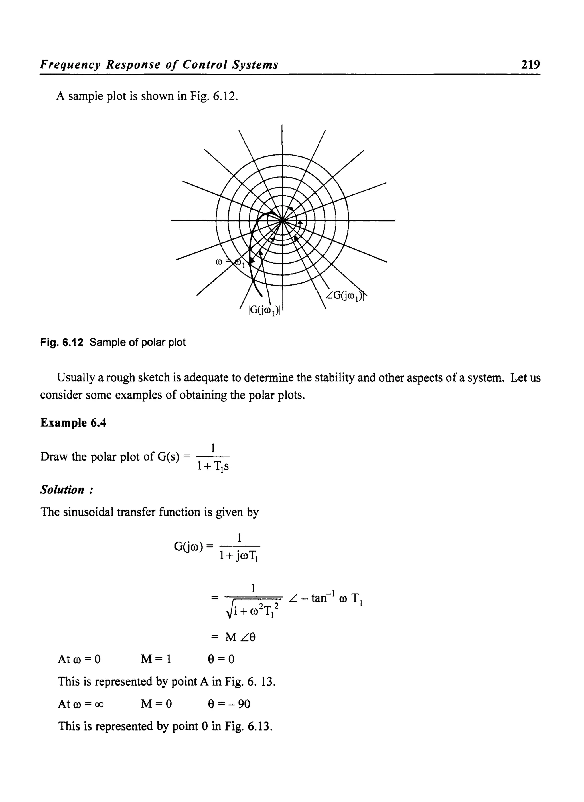
For any 0:::: co:::: 00, M:::: 1 and 0:::: e:::: - 90. In fact the locus of the magnitude of 10 Gco)1 can be
shown to be a semi circle. The complete polar plot is shown in Fig. 6.13.
o
00=00
1
Fig. 6.13 Polar plot of G(s) =--
l+Tl s
Example 6.S
1m GUm)
1
Draw the polar plot of O(s) = s(1 +TIs)
Solution:
At co = 0 o Gco) = - T] - j 00
= 00 L - 90°
---.00=0
A
At co = 00 o Gco) = - 0 - jO = 0 L -180°
the polar plot is sketched in Fig. 6.14.
1
Fig. 6.14 Polar plot of G(s) = - - -
s(1 +TIs)
1m GUm)
00=00
Re GUm)
Re GUm)

230. Frequency Response of Control Systems 221
Comparing the transfer functions of Exs. 6.4 and 6.5 we see that a pole at origin is added to the
transfer function of Ex. 6.4. The effect of addition of a pole at origin to a transfer function can be
seen by comparing the polar plots in Fig. 6.13 and 6.14. The plot in Fig. 6.13 is rotated by 90° in
clock wise direction both at ro = 0 and ro = 90°. At ro = 0 the angle is - 90° instead of 0 and at ro = 00
the angle is - 180° instead of - 90°. We say that the whole plot is rotated by 90° in clockwise
direction when a pole at origin is added.
A sketch of the polar plot of a given transfer functioIi•. can be drawn by finding its behaviour at
ro = 0 and ro = 00.
Example 6.6
Draw the polar plot ofG(s) = - - - - -
(1 +T]s)(1 + T2s)
Solution:
In this example, a non zero pole is added to the transfer function of example 6.4.
Let us examine the effect of this on the polar plot.
At ro = 0 . 1 I[G Oro)1 = M = (1 + jroT])(1 + jroT
2
) ro = 0 = 1
At ro = 00 [G Oro)[ = M = 0 L -180°
(Since ro = 00, the real part can be neglected and hence the magnitude is 0 and angle is - 180°)
The polar plot is sketched in Fig. 6.15.
Thus we see that the nature of the plot is unaffected at ro = 0 but the plot rotates by 90° in
clockwise direction at ro = 00.
Similarly ifa zero is added at some frequency, the polar plot will be rotated by 90 in anticlockwise
direction at ro = 00.
Im G(joo)
00 = co +-- 1 --.00 =0
1
Fig. 6.15 Polar plot of G(s) =-----(1 +T]s)(1 +T2s)

231. 222 Control Systems
Some examples of polar plots are shown in Fig. 6.16, which clearly demonstrate the aspect of
adding poles at origin and poles at other frequencies.
1m GUm) 1m GUm)
1
G(s) = - - - - -
s(l +Ts)(l +T2s)
1
G(s) - - - - - - - - -
(1 +Ts)(1 +T2s)(1 +T3S)
ReGUm) ReGUm)
m=O
CQ =0
(a) (b)
1m GUm) 1m GUm)
m=oo ReGUm) ReGUm)
(c) (d)
Fig. 6.16 Polar plot of some transfer functions.
6.5.3 Log Magnitude Vs Phase Plots
Another graphical representation of a transfer function is by plotting log magnitude of the transfer
function in db versus the phase angle at various frequencies. Usually the Bode plots are first obtained
and the magnitude in db and phase angle at a given frequency are read from them. Magnitude in db
is plotted against phase to obtain the log magnitude Vs phase angle plot as shown in Fig. 6.17
The advantages of these plots are that the relative stability can be determined with case and
compensators can be designed easily.

232. Frequency Response of Control Systems
Magnitude
in db
20
10
o
-10
-20
r'00
7
/f!
006
ei>~9.,; / ~oo = 0
1Sl....
)/'002
lro3
I °4
V
-300 -270 -240 -210 -180 -150 -120 -90
Phase angIe
Fig. 6.17 Log magnitude Vs phase angle.
6.6 All Pass Systems
223
A system which passes all frequencies without any attenuation is known as an all pass system or all
pass filter. Such systems are characterised by the transfer functions which have a zero in mirror
image position with respect to the imaginary axis ofs-plane for every pole in the left half ofs-plane.
We have seen in chapter 4, that for stable systems the poles must lie in the left halfofs-plane only. If
for every left half of s-plane pole there is a correspondinlS right half plane zero at mirror image
position, such a system is known as an all pass system. Consider the system,
I-Ts
G(s) =1+Ts
The pole zero locations are shown in Fig. 6.18.
1m s
-liT
Fig. 6.18 Pole zero pattern of all pass system.
For s = jOJ, magnitude of G(s) is
s-plane
liT Res
= 1

233. 224 Control Systems
The magnitude is independent of ro and hence it passes all frequencies with a gain of unity.
The angle of G Oro) is given by
LG Oro) = - 2 tan-
j
roT
As ro is increased from 0 to 00, the angle changes from 0 to - 1800
•
6.7 Minimum Phase Systems
A system with all zeros and poles in the left half of s-plane is known as a minimum phase function.
For a stable system all poles have to b~ necessarily in the left half ofs-planes. However, there is no
restriction on the zeros of the transfer function. Consider a system with one zero in the right half of
s-plane and two poles in the left half ofs-plane.
I-T s
G(s) - a
(1 +Tj s)(1 +T2s)
This can be written as
= Gj(s). Ga(s)
Here G(s) is considered as a product oftwo transfer functions Gj(s) and Ga(s). G1(s) has all poles
and zero in the left half of s-plane. GaCs) is an all pass system. Since the contribution of GaCs) to
magnitude of G(s) is unity, the magnitude plot ofG(s) and G/s) are identical. But the all pass system
contributes angles 0 to - 180 as m is changed from 0 to -180°, the angle of G(jm) will be more than
the angle of GjOm) for all frequencies. Thus G(jm) and GjOm) have same magnitude plots but
different phase angle plots. Thus it is evident that the phase angle of a transfer function could be
changed without affecting its magnitude characteristic, by adding an all pass system.
Hence for a given magnitude characteristic GjOm) has the least phase angle compared to G(jm).
Thus GjOm) which has all poles and zeros in left half plane is known as minimum phase system.
G(jm) which has one or more zeros in right half plane, but has the same magnitude plot is a non
minimum phase system. A minimum phase function has a unique magnitude, phase angle relationship.
For a non minimum phase function for a given magnitude characteristic, the phase angle is more
lagging than the minimum phase function.
These larger phase lags are usually detrimental to the system and hence they are avoided in control
systems. The phase angle characteristics of minimum, all pass and non minimum phase functions
Gj(s), Ga(s) and G(s) are shown in Fig. 6.19.

234. Frequency Response of Control Systems 225
____O~~~=-------------------logoo
G1 Goo)
_90+-____~~~----~======m=in;i=mumph~e
Ie GaGro)
+ ~___ all pass
-180~--------~~----------
-270~------------------~=-
Fig. 6.19 Phase angle characteristics of minimum phase, all pass and non minimum phase systems
For a given non minimum phase transfer function, it is always possible to get the corresponding
minimum phase function which has exactly the same magnitude characteristic but least phase angle
characteristic. To do this, for every right half plane zero of the given transfer function, associate an
all pass function and add a zero in the left half plane at corresponding position so that the magnitude
curve remains the same.
Consider
G(s)
(1- 2s)(1- 5s)
s(1 +3s)(1 +lOs)
(1 +2s)(1 +5s) ( 1- 2s ) (l - 5s)
s(l + 3s)(1 + 1Os)· 1+ 2s (l + 5s)
= Gl(s). Gal(s) Gais)
Gl(s) is required minimum phase function Gal(s) and Ga2 are all pass functions. Gl(s) has same
magnitude curve as G(s) but has the least phase angle curve.

235. 226 Control Systems
Problems
6.1 Find the frequency response specItications Mr, ror' rob for the systems with the following
closed loop transfer functions.
(a)
16
S2 +4.8s+16
(b)
32
s2+8s+32
(c)
100
S2 +16s+100
(d)
64
S2 +6.4s+64
6.2 For the following open loop transfer functions with unity feedback, draw the Bode plot and
determine the frequency at which the plot crosses the 0 db line.
2000
(a)
s(s + 2)(s + 100)
15(s + 5)
(b)
S(S2 + 16s + 100)
lOs
(c)
(O.ls + l)(O.Ols + 1)
6.3 Sketch the Bode flot for the following systems and determine the value of K for which the
magnitude plot crosses the 0 db line at ro = 15 rad/sec.
K(s +2)
(a) s(s + 4)(s + 10)
K
(b) s(1+s)(1+0.ls)(1+0.01s)

236. Frequency Response of Control Systems 227
6.4 The asymptotic approximation of the gain plot is given in the following figures. Obtain the
open loop transfer function in each case.
db
odb/dec
14 db - - - - - -"'"----------..
(a)
0.1 2 10 ~logO)
db
10 20 logO)
(b)
-14db - - - - - - - - - - - - -
6.5 The following data refers to the frequency response test conducted on an open loop system.
Plot the Bode magnitude plot and approximate by asymptotes to obtain the transfer function.
(0 rad/sec 0.2 0.5 1 1.5 2 2.5 4 5 8 10 20 50
Gain 9.85 6.68 1.57 0.914 0.62 0.46 0.25 0.19 0.1 0.072 0.022 0.004
6.6 For the following unity feedback system obtain the values ofK and 't to get a peak resonance
of 1.26 at a resonance frequency of 10.5 rad/sec.
K
G(s)- - -
s('ts +1)
Also find the peak overshoot and settling time for a unit step input.
6.7 Draw the frequency response curve of the following closed loop transfer function and
obtain Mr and (Or·
C(s) 540
R(s) (s + 15)(s2 + 4s + 36)
Where will the poles of equivalent second order system be located.

237. 228 Control Systems
6.8 Sketch the polar plots of the following open loop transfer functions. Find the frequency at
which the plot crosses the negative real axis and the magnitude of GUoo) at this frequency.
10
(a) (s +1)(s +3)
10
(b) s(s +1)(s +5)
10
(c) (s +1)(s +3)(s +5)
(1 +0.2s)
(d) s2(1 +O.Ols)(1 + 0.05s)
6.9 Sketch the polar plot of the function,
10
G(s) = s(s +5)(s +10)
For what value of 00, IGUoo)1 = 1. At this frequency what is the phase angle of GUoo).

238. 7 Nyquist Stability Creterion and
Closed Loop Frequency Response
7.1 Introduction
In chapter 4, it was shown that the location of the roots of the characteristic equation determines
whether a system is stable or not. Ifall the roots lie in the left half ofs-plane, the system is absolutely
stable. If simple roots are present on the imaginary axis of the s-plane, sustained oscillations in the
system will result. Using Routh Hurwitz criterion, a simple way of determining the roots in the right
halfofs-plane or on the imaginary axis was discussed. But Routh-Hurwitz criterion gives only absolute
stability but does not tell us about how much stable the system is i.e., it can n~t throw any light on
relative stability ofthe system. Root locus technique discussed in chapter 5, can be used to determine
the location ofclosed loop poles on the s-plane from the location of poles and zeros ofthe open loop
system when one parameter of the system, usually the gain, is varied. This also does not give a
measure of the relative stability of the system.
A frequency domain technique is developed in this chapter, which gives a simple way ofdetermining
the absolute stabilitY ofthe system, and also defines and determines the relative stability ofa system.
This frequency domain criterion is known as Nyquist Stability Criterion. This method relates the
location of the closed loop poles of the system with the frequency response of the open loop system.
It is a graphical technique and does not require the exact determination ofthe closed loop poles. Open
loop frequency response can be obtained by subjecting the system to a sinusoidal input of constant
amplitude and variable frequency and measuring the amplitude and phase angle of the output.
The development of Nyquist Criterion is based on a theorem due to Cauchy, 'the principle of
argument' in complex variable theory.

239. 230 Control Systems
7.2 Principle of Argument
Consider a function ofcomplex variable's', denoted by F(s), which can be described as a quotient of
two polynomials. Assuming that the two polynomials can be factored, we have
.....(7.1)
Since s = a +jOJ is a complex variable, for any given value of s, F(s) is also complex and can be
represented by F(s) = u +jv. For every point s in the s-plane at which F(s) and all its derivatives exist,
ie, for points at which F(s) is analytic, there is a corresponding point in the F(s) plane. It means that
F(s) in eqn. (7.1) maps points in s-plane at which F(s) is analytic into points in F(s) plane. In
eqn. (7.1) s = - PI's = - P2 are the poles of the function F(s) and therefore the function goes to
infinity at these points. These points are also called singular points of the function F(s).
Now, consider a contour .s in s-plane as shown in Fig. (7.1) (a). Assume that this contour does
not pass through any singular points of F(s). Therefore for every point on this contour, we can find
a corresponding point in F(s) plane, or corresponding to the contour .5 in s-plane there is a contour l'
in F(s) plane as shown in Fig. 7.1 (b).
jro
s-plane
'ts
S3
(j
Fig. 7.1 (a) Arbitrary contour 't. in s-plane not
passing through singular points of F(s)
jv F(s)-plane
--~----~--~---7U
Fig. 7.1 (b) Corresponding F(s)-plane
contour'tf
Let us consider a closed contour and define the region to the right of the contour, when it is
traversed in clockwise direction, to be enclosed by it. Thus the shaded region in Fig. 7.1(a) is considered
to be enclosed by the closed contour .s' Let us investigate some of the properties ofthe mapping of
this contour on to F(s)-plane when .s encloses (a) a zero of F(s) (b) a pole of F(s).
Case a: When .s encloses a zero of F(s)
Let s = -Zj be encloses by the contour .s as shown in Fig. (7.2) (a).
/ / ~.....
/ / (SI+P3) I
_p'X (SI+Z2) I
3 0
-Zz
Fig. 7.2 (a) Contour ts encloses one zero
s =Z1 of F(s)
jv
F(s)
F(s) plane
U
Fig. 7.2 (b) Corresponding F(s) plane
contour'tf

240. Nyquist stability criterion and closed loop frequency response 231
For any point s = sl' we have
.....(7.2)
where 0.1 = lSI + zd, 0.2 = lSI + ~I, ..... am = lSI + zml
PI = lSI + Pll, P2 = lSI + P21, •.•.• Pn = lSI + Pnl
and 91= /(sl + zl)' 92 = /(sl + ~), ..... 9m =[(Sl +~)
1>1 = /(Sl + PI)' 1>2 = [(Sl + P2)' ..... I>n =[(Sl + Pn)
In the development of Nyquist criterion the magnitude of F(s) is not important, as we will see
later. Let us concentrate on the angle of F(s).
In Fig. 7.2(a), as the point s moves on the contour 's in clockwise direction, and returns to the
starting point, let us compute the total angle described by F(s) vector as shown in Fig. 7.2(b).
The vector (s + zl) contributes a total angle of -27t to the angle of F(s) as shown in Fig. 7.3(a)
since the vector (s + zl) makes one complete rotation. This is because the point s = - zl lies inside the
contour.
jw
s-plane
Fig. 7.3 (a) Angle contributed by (s + Z1) to F(s)
The vector (s + Z2)' contributes zero net angle for one complete traversal of the point s on the
contour 's in s-plane as shown in Fig. 7.3(b). This is because the point s = - z2 lies outside the
contour 's'
jw
s-plane
Fig. 7.3 (b) Angle contributed by (s + Z2) to F(s)

241. 232 Control Systems
..
Similarly all the zeros and poles which are not enclosed by the contour 's' contribute net zero
angles to F(s) for one complete traversal ofa point s on the contour 's' Thus the total angle contributed
by all the poles and zeros of F(s) is equal to the angle contributed by the zero s = - zl which is
enclosed by the contour. The F(s) vector describes an angle of - 21t and therefore the tip of F(s)
vector describes a.closed contour about the origin of F(s) plane in the clockwise direction. Similarly
if k zeros are enclosed by the s-plane contour, the F(s) contour will encircle the origin k times in the
clockwise direction. Two cases for k = 2 and k = 0 are shown in the Fig. 7.4 (a) and (b).
s-plane
jro F(s) plane
x x
u
x x
Fig. 7.4 (a) s-plane contour and F(s) plane contour for k =2.
jro s-plane jv F(s) plane
x x
t
s
0' u
x
Fig. 7.4 (b) s-plane contour and F(s) plane contour for k =O.
Case b : When 'ts encloses a pole of F(s)
When a pole of F(s), s = -PI is enclosed by the contour 's' a net angle of21t is contributed by the
vector (s +PI) to F(s) as the factor (s +PI) is in the denominator ofF(s). Thus the F(s) plane contour
will encircle the origin once in the anticlockwise direction.
If s-plane contour 's encloses P poles and Z zeros, the F(s) plane contour encircles the origin
P times in the anticlockwise direction and Z times in the clockwise direction. In otherwords, it
encircles the origin of F(s) plane (P - Z) times in the anticlockwise direction. The magnitude and
hence the actual shape of the F(s) plane contour is not important, but the number of times the
contour encircles the origin is important in the development of Nyquist stability criterion, as will be
discussed in the next section. This relation between the number of poles and zeros enclosed by the
closed s-plane contour 's' and the number of encirclements of F(s) plane contour 't is known as the
principle ofArgument.

242. Nyquist stability criterion and closed loop frequency response
7.2.1 Nyquist Criterion
For a feedback control system with loop transfer function given by :
K(s + ZI)(S + Z2).····(S + Zm)
G(S) H(s) = m S n
(s + Pl)(S + P2)....·(S + Pn)
m
1t(S + ZJ
= K .!:i=:.!....l- -
n
1t(S+PJ)
J=1
The characteristic equation is given by
m
K 1t(s+z)
i=1
D(s) = I + G(s) H(s) = I + -n":""":-'-- = 0
.1t(s+p)
J=1
n m
1t (S + pj) + K 1t (s + Z )
J=1 1=1-"----n----- = 0
1t (S +PJ)
j=l
233
.....(7.3)
.....(7.4)
The numerator ofeqn. (7.4) is a polynomial of degree n and hence it can be factored and written as
(s + z;)(s + z;).....(s + z~)
D(s) = n = 0 .....(7.5)
1t(s+Pj)
J=1
Thus it can be observed that:
1. The poles of the open loop system G(s) H(s) and poles of D(s) are the same
(eqns. (7.3) and (7.5»
2. The roots of the characteristic equation D(s) = 0 are the zeros of D(s) given by -z;, -z;,....-z~
in eqn. (7.5).
3. The closed loop system will be stable ifall the poles ofthe closed loop system, ie, all the roots
ofthe characteristic equation lie in the left halfofs-plane. In otherwords, no pole ofthe closed
loop system should be in the right half ofs-plane.
4. From eqn. (7.4) and (7.5), it is clear that even if some poles of open loop transfer function
(-PI' -P2' ... -Pn) lie in right half of s plane, the closed loop poles, or the zeros ofD(s) = 0 ie
s = - z ;, - z; etc many all lie in the left half ofs-plane. Thus even if the open loop system is
unstable, the closed loop system may be stable.

243. 234 Control Systems
In order to detennine the stability of a closed loop system. we have to find if any of the zeros of
characteristic equation O(s) = 0 in eqn. (7.5) lie in the right half ofs-plane. Ifwe consider an s-plane
contour enclosing the entire right half of s-plane, plot the O(s) contour and find the number of
encirclements of the origin, we can find the number of poles and zeros of O(s) in the right half of
s-plane. Since the poles ofO(s) are the same as open loop poles, the number of right half plane poles
are known. Thus we can find the number of zeros of O(s) ie the number of closed loop poles in the
right half of s-plane. If this number is zero. then the closed loop system is stable, otherwise the
system is unstable.
7.3 Development of Nyquist Criterion
7.3.1 Nyquist Contour
Let us consider a closed contour, 'N which encloses the entire right half of s-plane as shown in
Fig. 7.5. This contour is known as a Nyquist Contour. It consists ofthe entirejaraxis and a semicircle
ofinfinite radius.
Fig. 7.5 Nyquist Contour
On the jeo-axis,
jco joo
-joo
s-plane
cr
s = jeo and eo varies from - 00 to + 00.
On the infinite semicircle,
s = It
R--+oo
'S 1t 1t
Rel , 8 varies from + - to 0 to - -
2 2
Thus the Nyquist Contour encloses the entire right halfofs-plane and is traversed in the clockwise
direction.
7.3.2 Nyquist Stability Criterion
If
n
1t(s + zJ
O(s) = ":"':..0.1_ __
,1t(s+p)
J=1
.....(7.6)
is plotted for values of s on the Nyquist contour, the O(s) plane contour will encircle the origin N
times in the counter clockwise direction, where
N=P-Z .....(7.7)
and P = number of poles of O(s) or the number of open loop poles in the right half of s-plane
(R.H.S)
Z = Number of zeros of O(s) or the number of closed loop poles in the RHS.

244. Nyquist stability criterion and closed loop frequency response
If the closed loop system is stable,
z==o
Thus, for a stable closed loop system,
N==P
235
.....(7.8)
i.e., the number of counter clockwise encirclements of origin by the O(s) contour must be equal to
the number of open loop poles in the right half ofs-plane. Further, ifthe open loop system is stable,
there are no poles of G(s) H(s) in the RHS and hence,
p==o
.. For stable closed loop system,
N==O
i.e., the number of encirclements of the origin by the O(s) contour must be zero.
Also observe that G(s) H(s) == [1 + G(s) H(s)] - 1
.....(7.9)
Thus G(s) H(s) contour and O(s) == 1 + G(s) H(s) differ by 1. If 1 is substracted from
O(s) == 1 + G(s) H (s) for every value ofs on the Nyquist Contour, G(s) H(s) contour will be obtained
and the origin of O(s) plane corresponds to the point (- 1, 0) of G(s) H(s) plane, this is shown
graphically in Fig. 7.6.
Im
D(s) = 1+GH-plane
GH-plane.
Re
Fig. 7.6 O(s) =1 + G,H plane and GH plane Contours
If G(s) H(s) is plotted instead of 1 + G(s) H(s), the G(s) H(s) plane contour corresponding to the
Nyquist Contour should encircle the (-1, jO) point P time in the counter clockwise direction,
where P is the number ofopen loop poles in the RHS. The Nyquist Criterion for stability can now be
stated as follows:
If the 'tGH Contour of the open loop transfer function G(s) H(s) corresponding to the Nyquist
Contour in the s-plane encircles the (-1, jO) point in the counter clockwise direction, as many times
as the number ofpoles ofG(s) H(s) in the right half ofs-p1ane, the closed loop system is stable. In the
more common special case, where the open loop system is also stable, the number of these
encirclements must be zero.

245. 236 Control Systems
7.3.3 Nyquist Contour When Open Loop Poles Occur on jro-axis
IfG(s) R(s) has poles on the jro-axis, 1+ G(s) R(s) also has these poles on the jro-axis. As the Nyquist
Contour defined in section 7.2.2 passes through these jro-axis poles, this Contour is not suitable for
the study of stability. No singulasitics of 1 + G(s) R(s) should lie on the s-plane Contour "s' In such
cases a small semicircle is taken around these poles on the jro-axis towards the RHS so that these
poles are bypassed. This is shown in Fig. 7.7.
jro
s-plane
(j
Fig. 7.7 Nyquist Contour when jro-axis poles are present
If an open loop pole is at s = ±jtVI, near this point, s is taken to vary as given be eqn. (7.10).
7t 7t
S = jrol + E~O E e19
, 8 changes from - "2 ~ 0 ~ "2 .....(7.10)
This describes the semicircle around the pole s = jtVl in the anti clockwise direction. Let us now
consider some examples illustrating how the Nyquist plots are constructed and the stability deduced.
Example 7.1
Let us obtain the Nyquist plot of a system whose open loop transfer function G(s) R(s) is given by
10
G(s) R(s) = (s + 2)(s + 4)
Solution:
The Nyquist path is shown in Fig. 7.8(a).
s-plane
o
(j
Fig. 7.8 (a) Nyquist path
Let us plot G(s) R(s) over the contour 't5
•

246. Nyquist stability criterion and closed loop frequency response
1. On the jro-axis if ro changes from 0 to +00
S = jro
10
IG(s) H(s)ls = JOl = (jro + 2)(jro + 4)
For ro = 0
For ro = 00
10
IG(s) H(s)1 = 8 = 1.25;
IG(s) H(s)1 = 0;
/G(s) H(s) = 0
/G(s) H(s) = -180°
237
As the exact shape of G(s) H(s) is not required we can draw this part of the GH Contour by
noting that the angle of GH changes from 0 to - 180 as ro changes from 0 to 00.
ImGH
GH plane
s = ao s=o
1.25 Re GH
Fig. 7.8 (b) Part of GH plot for s =jO to s =jao
2. For the infinite semi circle described by s =jooto 0 to s = -joo. For this part of the contour,
s = It R el9 e= 2: ~ 0 ~ _ 2:R-+<Xl 2 2
G(s) H(s) = _-;;--_1_0_-;;--_
(ReJ9
+2)(ReJ9
+ 4)
As R ~ 00, Rel9
» 2 and Rel9
» 4
10
G(s) H(s) = R!!~ = It r e-J29
~- R2 eJ29 r-+O
10
where r = RT and as R ~ 00, r ~ 0
1t 1t
As R ~ 00, IG(s) H(s)1 ~ 0 and as echanges from "2 to 0 to - "2
/G(s) H(s) = -1t to 0 to 1t
This part of the G(s) H(s) plot is shown in Fig. 7.8(c).
ImGH
GH plane
s =-jao s = ao
----------~~----------- ReGH
s =jao r -+ 0
Fig. 7.8 (c) Nyquist plot corresponding to the Nyquist path of infinite semicircle.

247. 238 Control Systems
3. For the Nyquist path on the jro-axis
At s = -joo
At s = jO
s = jro and ro = -00 to ro = 0,
10
G(s) H(s) = (jro+2)(jro+4)
10
G(s) H(s) = ( . )( . ) = 0 L+l80
-Joo -Joo
10
G(s) H(s) = (j0 + 2)(j0 + 4) = 1.25LO
This part ofthe Nyquist plot is shown in Fig. 7.9 (d). The angle changes from +180 to 0 as ro
changes from -00 to O.
ImGH
GH plane
ill = 0
ill =-00 ReGH
Fig. 7.9 (d) Nyquist plot for s = -jOCI to s = jO
The complete Nyquist plot for the contour 't
s is shown in Fig. 7.9(e).
ImGH
GH plane
1.25
ReGH
10
Fig. 7.9 (e) Complete Nyquist plot of G(s) H(s) =( (s+2) s+4)
The (-1, jO) point is also shown in the Fig. 7.9 (e), It is obvious that the Nyquist plot does not
encircle the point (-l,jO). Therefore N = 0 Since there are no poles ofG(s) H(s) in the right
halfofs-plane,
or
P=O
N=P-Z
O=O-Z
z=o
Thus there are no zeros of 1 + G(s) H(s), ie., poles ofthe closed loop system in the right half
of s-plane. Hence the system is stable.

248. Nyquist stability criterion and closed loop frequency response 239
Recall that G(s) H(s) is given by,
m
rc(s + zJ
1=1
G(s) H(s) = -'--n-'--- and m :s n.
rc(s+Zj)
j=1
For many practical systems m < n. For such systems the infinite semicircle always maps into
origin and the Nyquist plot goes round the origin with radius tending to zero. Since we are interested
in the encirclement of the point (-1, jO), this part of the Nyquist plot is not required for determining
the stability. Hence the mapping ofinfinite semicircle can be considered to be mapped on to the origin
of GH plane. Moreover, since
G* (jro) H* (jro) = G(-jro) H (-jro)
the GH plot is symmetrical about the real axis. Hence if GH plot is obtained for values of s on the
positive imaginary axis, the plot for values ofs on the negative imaginary axis will be its mirror image.
Therefore it is sufficient to plot the GH plot for s = jO to s = jcc. The infinite semi circle maps into
origin. The plot for s = -joo to s = 0 is the mirror image of its plot for s = jO to s = joo.
Example 7.2
Determine the stability of the system
10
G(s) H(s) = s(s + I)(s + 4)
Solution:
The Nyquist path is shown in Fig. 7.10(a).
Fig. 7.10 (a) Nyquist path
I. For points on positive jro axis
s = jro
1m s
0+ < ro < 00
10
For
G(s) H(s) = jro(jro+I)(jro+4)
s = jO+
10
Res
G(s) H(s) = jO(j0+1)(jO+4) = 00 L-90

249. 240 Control Systems
For s = joo
10
G(s) H(s) = . (. 1)(. 4) =0 L-270
Joo Joo + Joo +
This part of locus of G(s) H(s) corresponds to the curve ABO in Fig. 7.10(b).
2. The infinite semicircle maps on to the origin.
3. The locus of G(s) H(s) for s = -joo to s = jO on the negative imaginary axis corresponds to
curve OBC in Fig. 7.10(b).
10
Fig. 7.10 (b) Complete Nyquist plot of G(s) H(s) = - - - -
s(s +1)(s + 4)
4. For the semicircle s = E ei8
around the pole at the origin,
10
G(s) H(s) = , ,
E eJ8
(E eJ8
+1)(E eJ8
+ 4)
It E ei8
<< 1 and E ei8
<< 4E--+O
10
G(s) H(s) = It --,s
E--+O E eJ
As evaries from - ~ to 0 to ~
2 2
G(s) H(s) varies from 00 L ~ to 00 LO to 00 L-~
2 2
D
This part of the GH plot corresponds to the infinite semicircle CDA.
5. To determine stability, we need to know whether the Nyquist plot encircles the (-I,jO) point or
not. For this, we should determine where the locus crosses the negative real axis ie., the point
B. Since the point B lies on the locus corresponding to s = jOJ as ro changes from 0+ to 00, let us
find the value of ro at which the imaginary part of G(s) H(s) is equal to zero.
10
G(s) H(s)ls =JQ} = jro(jro + 1)(jro + 4)

250. Nyquist stability criterion and closed loop frequency response
Let us rationalise this and obtain its real and imaginary parts.
10(1- jro)(4 - jro)
G Oro) H Oro) = jro(1 + ro2)(16 + ro2)
or
10(4- ro2- j5ro)
j<O(l + ro2)(16 + ro2)
-50 . 10(4-ro2
)
= (1 + ro2
)(16+ ro2) - J <0(1 + ro2
)(16+ ro2
)
1m G Oro) H Oro) =0
10(4 - ro
2
) == 0
<0(1 + 0)2)(16 + ro2)
oi=4
0) = ± 2 rad/sec
At 0) = 2 rad/sec, we have,
G 02) H U2) = -50 = -0.5
(1 + 4)(16+ 4)
241
.....(7.9)
Thus the Nyquist locus crosses the negative real axis at -0.5 for 0) = ±2 rad/sec. Thus the Nyquist
plot is as shown in Fig. 7.10 (c) with the point (-1, jO) also indicated.
GH-plane
(-1, jO) ReGH
Fig. 7.10 (c) Nyquist plot with the critical point (-1, jO)
It is clear from the Fig. 7.1O(c), the (-1, jO) point is not encircled by the GH locus. Hence the
system is stable.
Example 7.3
Let us consider an example in which the open loop system has a pole in the right half of s-plane.
Consider the system
K
G(s) H(s) = (s + 2)(s -1)

251. 242
Solution:
The Nyquist path is as shown in Fig. 7.11(a).
joo
jill
o
-j00 '--------
Fig. 7.11 (a) Nyquist path.
1. As s changes on j<o axis,
At <0 = 0,
At <0 = 00,
s = j<o 0<<0<00
K
G(s) H(s) = U<o +2)U<o -1)
K K
GGO) H GO) = - - = - L 180
2 2
GG )HG ) K
00 00 = 000 +2)(j00 -1)
= 0 /180
Control Systems
S-plane
2. As s moves on infinite semicircle G(s) H(s) maps on to the origin ofGH-plane.
3. For s = jOJ and -<X) < <0 < 0 the GH plot is mirror image of the plot for 0 < <0 < 00
The complete plot is as shown in Fig. 7.11(b).
1m GH
GH plane
=-«J
=00
ReGH
. K
Fig. 7.11 (b) NyqUist plot of GH ={s +2)(s -1) .

252. Nyquist stability criterion and closed loop frequency response 243
K
The Nyquist plot encircles the (-1, jO) point once in anti clockwise direction, if 2 > 1 or K> 2,
as shown in the Fig. 7.11(c).
0) = 0
-K
-
2
Fig. 7.11 (c) Nyquist plot for K > 2
For K > 2, we have
N= 1
ImGH GH plane
ReGH
Since there is one pole of G(s) H(s) in the right half of s-plane
P=1
From
or
N=P-Z
1=I-Z
z=o
Therefore there are no closed loop poles in the RHS and hence the system is stable for K > 2.
If K < 2, the Nyquist plot is shown in Fig. 7.11(d).
ImGH
GH plane
ReGH
Fig. 7.11 (d) Nyquist plot for K < 2
Clearly, the Nyquist plot does not encircle (-1, jO) point and hence
N=O
P=1
N=P-Z
Z=P=1
There is one zero ofthe characteristic equation or equivalently, one pole of closed loop system in
the RHS and therefore, the closed loop system is unstable for K < 2.

253. 244 Control Systems
This examples illustrates the fact that, even if the open loop system is unstable the closed loop
system may be stable. If some of the open loop poles are in the RHS, for stability the Nyquist plot
should encircle the origin, in counter clockwise direction, as many times as there are RHP poles of
the openloop system.
Example 7.4
Obtain the range of values of K for which the system with open loop transfer function
is stable.
Solution:
K(s+ 1)
G(s) H(s) = s2(s+2)(s+4)
(i) For the Nyquist path shown in Fig. 7.12 (a) and for values of s on section I of the path
joo
~SectionII
Fig. 7.12 (a) Nyquist path for example 7.4
for
for
s = jro 0+ < ro < 00
K(jro + 1)
G Oro) H Oro) = Uro)2(jro + 2)Uro + 4)
K
G 00+) HOO+) = -
(j0)2
= 00 L-180o
ro=oo
" K(joo + 1)
GOoo)HOoo)=-(j-00~)2-(j~00~+-2-)U~'00-+-4-)
Kjoo
(jooi (joo)Uoo)
= 0 L-270
Section II

254. Nyquist stability criterion and closed loop frequency response
The segment of Nyquist plat near s =jO+ and s =joo is shown in Fig. 7.12 (b).
..ooL-1800
Fig. 7.12 (b) Part of Nyquist plot at s = jO+ and s = joo
ImGH
OL-2700
GH plane
ReGH
245
It is clear from the plot shown in Fig. (7.12) (b) that the plot has to cross the negative real axis for
some value ofs = jm. Let us find this point. At this point the imaginary part of GUm) HUm) should be
zero or the angle of GUm) HUm) = ±1800
Equating / GUm) HUm) = - 1800
m m
tan-l m- 180 - tan-l - - tan-l
- = - 180
2 4
m m
tan-l m= tan-l - + tan-l -
2 4
Taking tangent of the angles on both sides, we have,
tan (tan-
l
m) = tan (tan-1 ~ + tan-1 : )
m m
-+-
m=~
m2
1--
8
Simplifying and solving for m, we have,
At this value of m,
m= J2 rad/sec
1
K(1 +m2
)2
IGUm) HUm)1 = - ----'---I--'----I
m2
(m2
+4)2(m2
+4)2
1
K(1 + 2)2
-_ 1 1
2(2 + 4)2 (2 +16)2
= -0.0722K

255. 246 Control Systems
Thus the GH plot crosses the negative real axis at -O.0722K for s = j J2 .
(ii) For selection II
The GH plot maps on to the origin of GH plane.
(iii) For selection III
The GH plot is a mirror image of plot for ro = 0+ to 00.
(iv) For selection IV
ase~O
s = It e ei9
e.....O
1t 1t
e~--~o~-
2 2
K(eej9
+1)
G(s) H(s) = - - - - - - ' - - - - - -
e 2 ej29(eeJ9 +1)(eej9 +4)
K
G(s) H(s) = 4 It e2 ej29
e.....O
as echanges from - 2: ~ 0 ~ 2: on the semicircle around the origin.
2 2
G(s) H(s) changes from 001.J!:.. ~ 00 ~ ~ 00 1-1t.
The complete plot is shown in Fig. 7.12 (c),
1
for 0.0722 K < 1 or K < 0.0722 = 13.85
and 0.0722 K> 1
1
or K> - - = 13.85
0.0722
----- --------.......,,...- , /'~
/~ ImGH
'"'" GH plane /
/ ' /
/0) =jO- ~ /0) =jO-
I
0) = joo 0) = joo
0) =jO+
f 0) = -joo / ReGH
(-1, jO) 0.0722K f 0) =jO+ 0.0722 K
' O)=Ji / ' 0)= J2
'" /
'"'" /' -..,, ,...-
-----4-- --------
(i) K < 13.85 (ii) K> 13.85
Fig. 7.12 (c) Nyquist plot for example 7.4.
~
"-
I
/
/
~
/'
,/

256. Nyquist stability criterion and closed loop frequency response
From plot (i) of Fig. 7.12 (c), the point (-1, jO) is not encircled by the GH plot and
hence. N = 0
since P = 0
and N=P-Z
z=o
Thus the system is stable for K < 13.85
From plot (ii) of Fig. 7.12 (c), the point (-1, jO) is :ucircled twice in clockwise direction.
.. N=-2
and
P=O
N=P-Z
-2=-Z
Z=2
247
There are two zeros ofthe characteristic equation in the RHP and hence the system is unstable for
K> 13.85. The range of values ofK for which the system is stable, is given by,
0< K < 13.85
Example 7.5
Determine the stability of the system
K(s+2)2
G(s) H(s) = 3
S
Solution:
Consider the Nyquist Centour shown in Fig. 7.13 (a).
joo .
JO> s-plane
Section II
(J
Fig. 7.13 (a) Nyquist path for example 7.5
The open loop system has a triple pole at the origin and Nyquist path is taken with an indentation
around the origin with a semi circle to bypass these poles.
Section I
s = jc.o c.o ~ 0+ t 0 00

257. 248 Control Systems
K(jro + 2)2
GUro) H Gro) = (jro)3
for ro = 0+
for ro=oo
K(joo+ 2i
GGoo) H Goo) = (joo)3 = 0 L-90
As the plot goes from - 270° to -90°, it has to cross the negative real axis for some value ro. At this
value of ro the imaginary part of GUro) HUro) should be zero.
. . K(jro + 2)2
GUro)HGro)= (jro)3
K(-ro2
+4+4jro)
_ jro3
jK(4-ro2
) 4K
ro3 - ro2
Equating the imaginary part to zero, we have
K(4- ro2
)
----'"---::----'- = 0
ro3
or ro2
= 4
and
ro = ± 2 rad/sec
IG Uro) H Uro)1 = - 4 K = - K
4
The Nyquist plot for section I of the Nyquist plot is shown in Fig. 7.13 (b).
GH plane
-K ReGH
Fig. 7.13 (b) Nyquist plot for section I of Nyquist path.

258. Nyquist stability criterion and closed loop frequency response
Section II
For values of s on this section the plot of GH will map on to the origin.
Section III
For this section the plot is mirror image of plot for Section I.
Section IV
On this section,
s = It E el9
e-+O
1t 1t
e~--~o~-
2 2
K(EeJ9 + 2)2
G(s) H(s)s = Eej9 = (E eJa)3
As E ~o
4K '39
G(s) H(s) = --,- = cJ:) e-J
E3 eJ39
For different values of e, LG(s) H(S)i J'e is tabulated.
S=Ee
Table 7.1
e LG(s) H(s)
-90 + 270
-60 + 180
-30 + 90
0 0
30 - 90
,+ 60 - 180
90 - 270
The plot of G(s) H(s) for this section is shown in Fig. 7.13 (c).
GH plane
00 L-lSO 00 LO
ReGH
00 L-90
Fig. 7.13 (c) Plot of GH for Section IV.
249

259. 250 Control Systems
The complete Nyquist plot is shown in Fig. 7.13 (d).
Q) = 0+
GH plane
ReGH
K(s + 2)2
Fig. 7.13 (d) Complete Nyquist plot of G(s) H(s) = 3
S
For K > 1, the point (-1, jO) is traversed once in anticlockwise direction and once in clockwise
direction as can be seen for Fig. 7.13 (d). The net encirclements are zero and since there are no poles
in the right half of s-plane, the system is stable.
For K > 1, the point (-1, jO) is traversed twice in clockwise direction and therefore,
N=-2
Since
and
P=O
N=P-Z
-2=0-Z
Z=2
The system is unstable.
Example 7.6
Comment on the stability of the system.
Solution:
K(s +10)(s + 2)
G(s) H(s) = (s +O.5)(s - 2)
The Nyquist path consists ofthe entire jro axis and the infinite semicircle enclosing the right half of
s-plane.
For
for
s = jro and ro ~ 0 to 00
K(jro +1O)(jro + 2)
G(s) H(s) = (jro +0.5)(jro - 2)
ro=O
20k
G(s) H(s) = - = - 20k = 20KL180
-1

260. Nyquist stability criterion and closed loop frequency response
for co =00
G(s) H(s)= It00.....0
=K
To find the possible crossing of negative real axis,
1m G (jco) H (jco) = 0
K(jco + 1O)(jco + 2)(- jco + 0.5)(-jco - 2)
1m =0
(co2 + 0.25)(co2 + 4)
1m (_co2
+ 20 + 12jco)(-o? - 1 + 1.5jco) = 0
-1.5co2
+ 30 - 12 - 12co2
= 0
IS 4
co2 = --=-
13.5 3
co = 1.1547 rad/sec
Re [G(jco) H(jco)]0) =11547 =
K -(20-C0
2
)(1+co
2
)-ISoo
2
1
(co
2
+.25)(co
2
+4) 00=11547
-SK
Hence the Nyquist plot crosses the negative real axis at - SK for co = 1.1547 rad/sec.
251
The infinite semicircle ofNyquist path maps into the origin of GH plane. The negative imaginary
axis maps into a mirror image ofthe Nyquist plot ofthe positive jco axis. Hence the complete Nyquist
plot is shown in Fig. 7.14.
1.9 K
ro=6.126
Fig. 7.14 Complete Nyquist plot of system in example 7.6.
By equating the real part of G(jco) H(jco) to zero, we can get the crossing ofjco-axis also. The plot
crosses the jco-axis at IG(jco) H(jco)1 = -1.9 K for co = 6.126 rad/sec. This is also indicated in the Fig.
7.14. From Fig. 7.14 it is clear that if SK > 1 or K > 0.125, (-1, jO) point is encircled once in
anticlockwise direction and hence
N= 1

261. 252
Since
and
P=1
N=P-Z
z=o
The system is stable for K > 0.125.
Control Systems
IfK < 0.125, the (-1, jO) point is encircled once in the clockwise direction and hence N =-1
Since
and
P=1
N=P-Z
Z=2
There are two closed loop poles in the RHP and hence the system is unstable.
7.3.4 Nyquist Stability Criterion for Systems which are Open Loop Stable
When the open loop transfer function does not contain any poles in the RHP we have P = 0 and for
stability N = 0 ie., there should not be any encirclements of (-1, jO) point by the Nyquist plot. The
Nyquist criterion can be simplified for all such cases and we can avoid drawing the entire Nyquist
plot. It is sufficient to draw the plot for points on the positive jro axis of s-plane and conclude about
the stability. In otherwords, the polar plot discussed in section 6.5.2 is sufficient to determine the
stability of open loop stable control systems.
Consider the Nyquist plot shown in Fig. 7.l0(c) for the system,
10
G(s) H(s) = s(s +1)(s + 4)
The system is open loop stable. The Nyquist plot is repeated in Fig. 7.l5(a) for convenience
GH-plane
m=2
(-l,jO) -0.5 ReGH
10
Fig. 7.15 (a) Nyquist plot of G(s) H(s) = s(s +1)(s + 4)
It is clear that the (-1, jO) point is not encircled by the Nyquist plot and hence the system is stable.

262. Nyquist stability criterion and closed loop frequency response 253
Let us now consider the portion ofthe plot for (j) = 0+ to (j) = 00 and the point (-I, jO) as shown in
Fig. 7.IS (b).
ImGH
B
(-1.jO)
to
Fig. 7.15 (b) Polar plot of the system G(s) H(s) = s(s+I)(s+4)
Let us define the term, 'enclosed'.
GH plane
ReGH
A point or region is said to be enclosed by a closed path ifit is found to lie to the right ofthe path
when the path is traversed in a prescribed direction. For example. shaded regions shown in
Fig. 7.IS (c) and 7.IS (d) are said to be enclosed by the closed contour. The point A is said to be
enclosed by the contour 't in Fig. 7.IS (c) but the point B in Fig. 7.IS (d) is not enclosed by 'to The
point C outside the path in Fig. 7.IS (c) is enclosed.
Fig. 7.15 (c) Point A enclosed by't. (d) Point B not enclosed but point C enclosed by't.
The point A in Fig. 7.IS(c) is encircled by the contour 't in clockwise direction, and the point is
also enclosed by the contour. In Fig. 7.IS(d), the point B is encircled by the contour 't in counter
clockwise direction but it is not enclosed, whereas the point C is not encircled by the contour 't, but
it is enclosed by the contour 'to
Now, coming to the discussion about the stability ofopen loop systems, it is clear that the Nyquist
Contour should not encircle the (-I, jO) point, for the system to be stable. In Fig. 7.IS(a) it can be
seen that for stable system (-I, jO) point should not be enclosed by the Nyquist contour. If we
consider the plot for (j) = 0 to (j) = 00 as shown in Fig. 7.IS(b), if the point (-I, jO) is not enclosed by
the plot, then the system is stable.
Thus the Nyquist Criterion in the case of open loop stable systems can be stated as follows:
The Nyquist plot for (j) = 0 to (j) = 00 (ie., the polar plot ofG(s) H(s)) should not enclose the point
(-1, jO) point when the plot is traversed in the indicated direction from (j) = 0 to (j) = 00. The point
(-1, jO) is known as the critical point.

263. 254 Control Systems
For an unstable system the point (-1, jO) will be enclosed by the polar plot as shown in Fig. 7.16.
ImGH
GH plane
ReGH
Fig. 7.16 Nyquist plot for an unstable system.
The polar plot, which can be obtained by conducting a frequency response test on the given
system, can be used to determine the stability of the system.
7.4 Relative Stability
So far we have considered only the absolute stability of the system. The Nyquist criterion tells us
whether the system is stable or not by the location of the critical point with respect to the Nyquist
plot. But often we are interested in knowing how stable the system is, if it is already stable. This
aspect of stability is known as relative stability of the system.
Consider a third order system given by
K
G(s) H(s) = s(s + l)(s + 4)
Consider the plot for four different values of K.
(i) K = 30
The polar plot of the system and its time response for a unit step input are as shown in
Fig. 7.17 (a) and (b) respectively.
ImGH
1.0
0) =0
-1.5 ReGH
c(t)
Fig. 7.17 (a) Polar plot of GH for K = 30 (b) Step response for K = 30
The polar plot shows that the (-1, jO) point is enclosed and hence the system is unstable. The
step response of this system increases with time.

264. Nyquist stability criterion and closed loop frequency response
(ii) K == 20
The polar plot for this case and its step response are shown in Fig. 7.18(a) and (b)
ImGH
c(t)
ro=oo 1.0
(-I,jO) ReGH
Fig. 7.18 (a) Polar plot of with K=20 (d) Step response for K =20
255
The polar plot passes through the critical point and the step response is purely oscillatory,
which corresponds to closed loop poles on the jro-axis. Thus, if the polar plot passes through
(-1. jO), the poles of the closed system lie on the jro axis and the system is marginally or
limitedly stable.
(iii) K == 15
The polar plot and the step response are shown in Fig. 7.19 (a) and (b) respectively.
ImGH
1.0
ro=oo
ReGH
~t
Fig. 7.19 (a) Polar plot of with K = 15 (b) Step response for K = 15
The system is stable for K == 15 but the point (-1, jO) is very near to the GH plot. The step
response is highly oscillatory and has large overshoot.
(iv) K == 10
The polar plot and the step response are as sketched in Fig. 7.20 (a) and (b) respectively.
ImGH
1.0
ro=oo
(-l.jO) ReGH c(t)
~t
ro=O
Fig. 7.20 (a) Polar plot of with K = 10 (b) Step response for K = 10

265. 256 Control Systems
The GH plot is far away from the critical point and the step response has less oscillations and low
overshoot.
From the above discussion it is clear that the system is more stable if the critical point (-1, jO) is
far away from the GH plot. Thus, the distance between the critical point and the GH plot can be used
to quantitatively obtain the relative stability of a system. It is to be noted that the relative stability
studies are made on open loop stable systems only.
7.4.1 Measures of Relative Stability: Gain Margin
We have seen that the nearness ofthe critical point (-1, jO) to the GH plot can be used to quantize the
relative stability of a system. One such measure is the "Gain Margin".
Consider the polar plot shown in Fig. 7.21. The point where the G(s) H(s) plot crosses the
negative real axis is known as the phase cross over frequency.
, ImGH
ReGH
Fig. 7.21 Polar plot and the phase cross over frequency.
At Cl) = rop~ the G(s) H(s) plot crosses the negative real axis, i.e, the phase angle changes from
-180° to + 180 . This frequency is therefore called as phase crossover frequency rope' The magnitude of
G(s) H(s) at s = jrope is given by OP and is equal to IG Grope) H Grope)l. The gain margin is defined as
1 1
Gain Margin (GM) = iG(jropc)H(jrope)i=-;;: .....(7.10)
Usually gain margin is specified in terms of decibels, db, as
1
Gain margin in db
1
=2010g10 -;;: •••••(7.11)
If a > 1, the GM is negative, the polar plot encloses the critical point and the system is unstable.
The system is more and more stable if the phase cross over point P is nearer and nearer to the origin.
The gain margin is positive for stable systems.
The magnitude of GGro) HGro) at any frequency ro, in particular at ro = ro e' will increase, as the
loop gain K is increased. Thus the phase cross over point P moves nearer to the criticaL point, as the
gain K is increased. For a particular value of K the value IG Grope) H Grope)1 becomes unity and the
system will be on the verge of instability.

266. Nyquist stability criterion and closed loop frequency response 257
Thus the gain margin can also be defined as the amount of increase in the gain that can be
permitted before the system becomes unstable.
I
From eqn. (7.10), if the gain is increased by ;-' IG Gcopc) H Gcopc)1 = I and the system will be on
the verge of instability. Now consider two systems with polar plots as shown in Fig. 7.22.
ImGH
(0=00
ReGH
Fig. 7.22 Polar plots of two systems with same Gain Margin.
The two systems have the same cross over point a and hence the two systems have the same gain
margin. But the system II is nearer to the critical point than the system I at some other frequency and
therefore the system I is relatively more stable than the system II, even though they both have the
same gain margin. Hence we need another factor to judge the relative stability of a system and is
defined as phase margin.
7.4.2 Phase Margin
Consider the polar plot shown in Fig. 7.23. Draw a circle with origin as centre and unit radius.
ImGH
(0 = 0
Fig. 7.23 Definition of gain cross over frequency and phase margin.
The frequency at which the polar plot crosses the unit circle, is known as Gain cross over
frequency, COgc' For frequencies greater than COgc' the magnitude of G(s) H(s) becomes less than
unity. If now an additional phase lag of $ = 180 - LG Gcogc) H Gcogc) = 180 - 8 is added without
changing the magnitude at this frequency, the polar plot ofthe system will cross (-I, jO) point. If the
polar plot is rotated by an angle equal to $ in the clockwise direction, the system becomes unstable.
Therefore, the phase margin can be defined as follows.
"Phase margin is the amount ofphase lag that can be introduced into the system at the gain cross
over frequency to bring the system to the verge ofinstability".

267. 258 Control Systems
The phase margin is measured positively from the -180° line in the counter clockwise direction.
The phase margin is positive for stable systems.
The value of the phase margin is given by
PM ~ = LG GOOge) H GoogJ + 180
where the angle of G GoogJ H GOOge) is measured negatively.
Gain Margin and phase margin are the two relative stability measures which are usually specified
as frequency response specifications. These specifications are valid only for open loop stable systems.
A large value of gain margin or phase margin denotes a highly stable system but usually a very slow
system. On the other hand a small value of either of these indicates a highly oscillatory system.
Systems with a gain margin ofabout 5 to 10 db and a phase margin ofaround 30 to 40° are considered
to be reasonably stable systems.
For many practical systems a good gain margin ensures a good phase margin also. But there may
be systems with good gain margin but low phase margin and vice vasa as shown in Fig. 7.24 (a)
and (b).
ImGH
........
"-
ro=<XJ
ReGH
Fig. 7.24 (a) System with good gain margin but low phase margin.
(b) System with good phase margin but poor gain margin
ImGH
ReGH
For a second order system, the polar plot does not cross the negative real axis at all, for any value
of gain K, as shown in Fig. 7.25. Hence the gain margin of such a system is infinity.
ImGH
....-
/
I
ReGH
Fig. 7.25 Polar plot of second order system for different values of gain
But the phase margin reduces as the value of K is increased. Thus for a second order system the
appropriate relative stability measure is the phase margin rather than the gain margin. Hence usually
phase margin is specified as one of the frequency domain specifications in the design of a control
system rather than the gain margin.

268. Nyquist stability criterion and closed loop frequency response
Example 7.7
Consider a unity feedback system with
K
G(s) - - - - - - -
s(0.5s + 1)(0.05s + 1)
Let us find the gain margin and phase margin for K = 1.
(a) Gain Margin
The polar plot ofG(s) is shown in Fig. 7.26.
ImGH
-.......
~
ill = 0
Fig. 7.26 Polar plot of G(s) H(s)
"-
J Re GH
/
/
259
To obtain the phase cross over frequency we will equate the imaginary part of GUro) to zero.
1
GUro) = jro(0.5jro +1)(0.05jm +1)
1
- 0.55ro2
+ jro(I - 0.025ro2
)
1m GUm) = 1 - 0.025 ro2
= 0
1
ro~e = 0.025 = 40
rope = ± J40
rope = 6.325 rad/sec.
At this frequency, the real part of GUro) is
. 1
Re GUrope) = - 0.55 x 40
= - 0.0454
The GH plot crosses negative real axis at -0.0454 for rope = 6.325 rad/sec.
Thus a = 0.0454
1
and GM = 20 leg -
a
1
= 20 log 0.0454
= 26.86 db

269. 260 Control Systems
The gain can be increased by a factor of ~ = 0.0454 = 22 for the system to remain stable.
(b) Phase Margin
Let us first fmd the gain cross over frequency. At this frequency, the gain is unity.
IGUm) HUm)1 = 1
1
----;r======--r===== = 1
m~1 + O.25m2 ~1 +O.0025m2
ie., m2 (l + O.25(2) (1 + O.OO25(2) = 1
Solving for m2 we get
and
m2 = 0.91
mgc = 0.954 rad/sec
LGUmgJ = - 90 - tan-I 0.5mgc - tan-I 0.05 mgc
=-118.232°
Thus phase margin is
~ = -118.232 + 180
= 61.768°
7.4.3 Adjustment of Gain K for Desired Values of Gain and Phase Margins Using
Polar Plots
We can also calculate the required gain K to obtain a specified gain margin and phase margin for a
given system.
Consider the Ex 7.7 again.
(a) Let the gain margin desired be 15db.
1
GM = 20 log - = 15
a
:. a=0.1778
For K = 1 the intercept was 0.0454. To get an intercept of 0.1778, we increase the gain by a
facts 0.1778/0.0454.
:. K = 3.92
(b) Let the phase margin desired be 45°. Then from definition,
LGUmgc) + 180 = PM = ~
- 90 - tan-I 0.5m - tan-I 0.05m + 180 = 45
Taking tangent of the angles on both sides, we have,
0.55m
- - - - , c - = tan 45 = 1
1-0.025m2
0.025m2 + 0.55m - 1 = 0
mgc = 1.69 rad/sec

270. Nyquist stability criterion and closed loop frequency response 261
At this frequency IGGrogc)1 = 1
K
--;:====,...-,====== = 1
1.69Jl + 0.25 x 1.692
Jl + 0.0025 x 1.692
K= 2.22
Thus ifK is increased to 2.22, the phase margin will be 45°.
Note: Gain and phase margins can be adjusted to the desired values analytically, only for
systems upto second order or third order, ifone ofthe three open loop poles occur at the origin
and there are no open loop zeros. Otherwise graphical procedure must be used to solve the
problem.
7.4.4 Gain Margin and Phase Margin Using Bode Plot
Bode plot also can be used to determine the gain and phase margins of a system and adjust the gain
for a given gain margin or phase margin. Let us first consider how phase and gain margins could be
determined using the Bode plot.
Example 7.8
Determine gain and phase margin for the unity feedback system using Bode plot.
10
G(s) = s(0.5s + 1)(0.05s +1)
Solution:
The Bode magnitude and phase angle plots are shown in Fig. 7.27.
When the phase angle curve crosses the -180° line, the frequency is read from the Bode phase
angle curve. This is phase crossover frequency ropc' At this frequency the magnitude in db is read
from the magnitude curve. This is the gain margin of the system. If at ropc' the gain is positive, it
means that IGGro) HGro)1 is greater than 1 and hence the system is unstable. Ifat the phase cross over
frequency the gain ofthe system is zero, the system is oscillatory. Finally ifat ropc the gain is negative,
IGGropc)1 < 1 and hence the system .is stable.
Similarly, the frequency at which the gain curve crosses 0 db line, is the gain cross over frequency,
ro c' At this frequency the angle of GGro) HGro) can be read off from the phase angle curve. Thang .
Phase margin ~ = !GGrogc) HGrogc) + 180
The angle of GGro~c) HGrogc) read above the -180° line gives the phase margin for a stable system.
If the angle ofGGro~c) HGrogc) lies below the - 180°, the phase margin is taken as negative and the
system will be unstable.
In the example 7.8.
and
and
ropc = 6.4 rad/sec
GM=8db
rogc = 4 rad/sec
PM = ~ = 15°

271. 262 Control Systems
40
~
I III I I I I I II
Uncompensated,
~ - - - Lag compensated
'r.::--t--.
jill / /11r--r--
20
10
~ G(s) H(s) = s(O.5s +1)(0.05s +1)
'~
o
~(Ogc
0.1 1.0 ~
,
10.0 100
I'll
J r---GM = 8db
~
'~
·20
-
r--r-.... r--..-40
r- ~
~ ~~
I'.
·60
"
I'~~
$pm = 5
~I ~
(Ope
~~
I.
~
"..... 1"-
~
Fig. 7.27 Bode plot for the system in Ex. 7.8
The system gain could be adjusted to a desired value using Bode plot.
Let us consider an example to illustrate this procedure.
Example 7.9
I.
Determine the gain and phase margin for the unity feedback system with K = 1.
K
G(s) s (0.5s +1)(0.05s +1)
'
·9
120"
150"
/ G
180"
210"
2
2700

272. Nyquist stability criterion and closed loop frequency response
Determine the value ofK for obtaining (a) gain margin of20 db (b) phase margin of 40°
Solution:
With K = 1, the magnitude and phase plots are drawn in Fig. 7.28.
4
3
0
11III .l I I I 1.1
0 Uncompensated
~
- - - Lag compensated
.V~ ~
~~ ~~
0 ....
~~
~~
~ (0 2=1.9... ge (0
00.1
... J. pe!
(Oge! = 0.9
~
10.0 100
t--- GM2= 20db(K = 2)
0
.~ '~ I I I I I"
~
1~I'-I - GM! = 26db(K = 1)
0
~~ I I"-0
~
K= 1
r- r--.0
" f'
~
~I-I--K=2
2
-1
-2
-3
-4
~ .~
~
1' r1
~ m =630 I.
" ~
400 ~ ~ ,
'"1
(Ogc
'"'
I.
'
~
I'
"
~
Fig.7.28 Bode plot for the system in.Ex. 7.e
263
-
1200
1
/ G
1sO"
2100
2
2700

273. 264 Control Systems
From the figure
O)gc 0.9 rad/sec.
~PM 63°
O)pe 6 rad/sec
GM 26 db
(i) To obtain a gain margin of20db, the gain ofthe system should be increased by (26 - 20) = 6db
without changing the phase cross over frequency, ie, the gain K must be increased such that
20 log K = 6
or K = 1.995 ::: 2
By making K = 2, the entire gain curve is shifted up by 6db. The phase curve is unaltered. The
gain curve for K = 2 is shown in Fig. 7.28.
(ii) To obtain a phase margin of40°, locate the frequency at which the phase curve has an angle of
(-180 + 40) = -140°. Find the gain at this frequency. Increase the value of K so that the gain
curve crosses 0 db line at this frequency.
From Fig. 7.28, -140° phase angle is obtained at a frequency of 1.9 rad/sec. This should be the
new gain cross over frequency when the K is increased.
O)gc (new) = 1.9 rad/sec.
At this frequency, the gain is read off from the magnitude plot for K = 1.
Gain at O)gc (new) = 8db
20 log K = 8
K = 2.51
Thus to get a phase margin of 40°, the gain should be increased to 2.51.
Note: Increasing the gain from K = 1 to K = K) means shifting the entire gain curve up by 20
log K) db. It is equivalent to shifting the 0 db line down by the same amount.Thus ifBode plot
for K = 1 is known.the gain margin and phase margin for a given value ofK = K) can be found
out shifting the 0 db line down by 20 log K db. The new gain cross over frequency and hence
the new phase margin can be read from the curves. At the phase cross over frequency which
remains same for K = 1 and K = Kl' the new gain margin can be found.
7.5 Closed Loop Frequency Response
Usually we are interested in the time response ofa control system. But this is often difficult to obtain.
On the otherhand frequency response ofa system could be obtained more easily. Bode plots and polar
plots could be used to represent them graphically. In chapter 6, we have shown that the frequency
response and time response are correlated to one another for a second order system. If time domain
specifications are given, frequency domain specifications can be easily obtained. The design of a
controller or compensator is carried out in frequency domain. The frequency response of the
compensated system can now be translated back to estimate the time response. Let us consider the
frequency domain specifications of a control system.

274. c
Nyquist stability criterion and closed loop frequency response 265
1. Resonance peak, Mr : This is the maximum of the magnitude of the closed loop frequency
response. From chapter 6, eqn. (6.8)
1
M = ---===
r 20~1- 02
It is seen that, Mr solely depends on the damping factor O. A small value of 0 corresponds to
large overshoot in time response and large resonance peak in frequency response.
2. Resonance frequency, OJr : This is the frequency at which resonance peak occurs.
From eqn. (6.7)
Resonance frequency is dependent on OJn and 0 and hence it is indicative of frequency of
oscillations and speed of response of the time response.
3. Bandwidth, OJd : It is defined as the range of frequencies for which the magnitude of the
frequency response is more than -3db. The frequency at which the gain is -3db, is known as
the cut offfrequency. Signals with frequencies above this frequency are attenuated. Bandwidth
is a measure of the ability of the system to reproduce the input signals in the output. It also
throws light on noise rejection capabilities ofthe system. More significantly it indicates the rise
time of time response of the system for a given damping factor. Fast response or small rise
time is obtained for systems with large bandwidth.
4. Cutoffrate: The rate of change of magnitude curve of the Bode plot at the cut off frequency
is known as the cut off rate. This is indicative of the ability of the system to distinguish
between signal and noise. However, sharp cut off often results in large resonance peak and
hence less stable system.
5. Gain margin andphase margin: These are the relative stability measures and are indicative
ofthe nearness of the closed loop poles to the jro axis. Usually phase margin, rather than gain
margin, is specified as one ofthe frequency domain specifications. The phase margin is directly
related to the damping factor, 0 for a second order system. Let us derive the relationship
between phase margin and the damping factor.
Consider a standard second order system with
G(s) H(s) = s(s+20ro
n
)
ro2
GGro)HGro)= . (. n
2
1: )
Jro Jro + uron
.....(7.12)

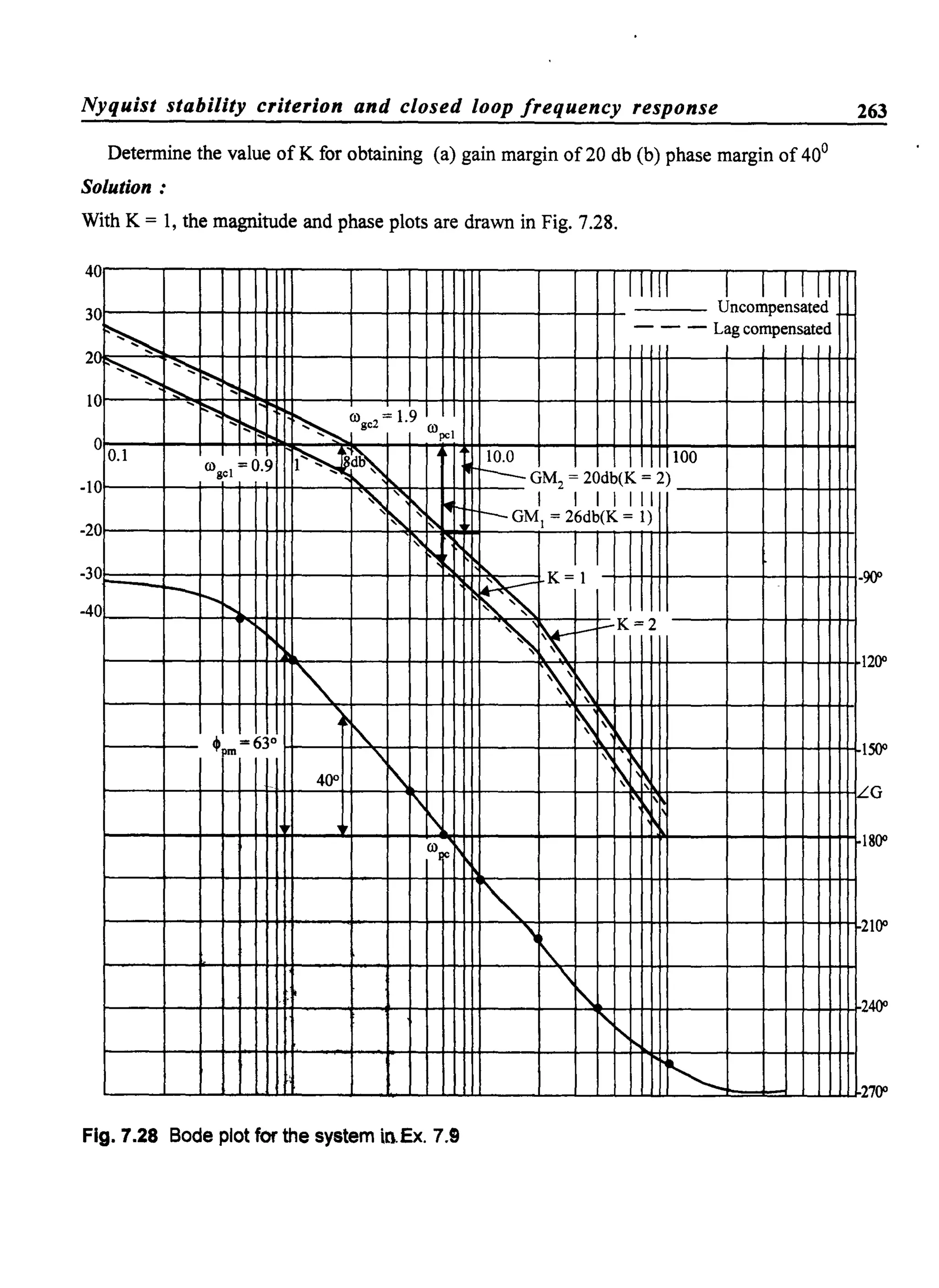
275. 266
At the gain cross over frequency cogc' IGUco) HUco)1 = 1
or co4
+ 402
co2
co2
- co4
= 0gc gc n n
This is a quadratic in co~c and the solution yields,
co2 = co2 ~(404 +1) _ 202
gc n
Phase margin of the system is given by,
_ COgc
~ = - 90 - tan - - + 180
pm 20con
tan ~pm = tan (90 - tan- ~l20con
_ COgc __ 20wn
= cot tan
20wn Wgc
_ 20wn
~ =tan - -pm CO
gc
From eqn. (7.13), we have
COn
Wgc = ~J404+1- 202
Substituting eqn. (7.16) in eqn. (7. 15),we have,
~pm~tan-I [ ~J4S':81-28']
Control Systems
.....(7.13)
.....(7.14)
.....(7.15)
.....(7.16)
.....(7.17)

276. Nyquist stability criterion and closed loop frequency response 267
Eqn. (7.17) gives a relationship between the phase margin and the damping factor for a second
order system for (3 < 1. Eqn. (7.17) is plotted for (3 ranging for 0 to 0.8 in Fig. 7.29.
0.8
0.6
1)
0.4
0.2
20 40 60 80 ~pm
Fig. 7.29 Curve showing the variation of ~pm with 8 for a scond order system.
As seen from Fig. 7.29, for values of 8 < 0.7 the curve is seen to be linear and hence can be
approximate by a straight line,
(3 = O.Ol~pm .....(7.18)
Here ~pm is to be taken in degrees.
Frequency response can be obtained for a given system to estimate the resonant peak and resonance
frequency which are the two important frequency domain specifications. But this is often difficult.
Thus graphical techniques are developed to determine ~ and ror from the open loop frequency
response.
7.5.1 Constant M Circles
Consider the polar plot ofthe open loop transfer function of a unity feedback system. A point on the
polar plot is given by :
G(s)ls =JCO = GUro) = x + jy.
The closed loop frequency response is given by
Let
C(jro) G(jro) x + jy
TUro) = R(jro) = 1+ G(jro) = I + x + jy
x
2
+/
IT Uro)12 - ------::~-=­
- (1 + X)2 + y2
IT Uro)1 = M
x2 +y2
M2 - --~--::­
- (l + X)2 + y2
M2 (1 + xi + M2 r= x2 + r
.....(7.19)

277. 268 Control Systems
Rearranging, we have
x2 (M2- 1) + 2xM2 + i (M2- 1) = _M2
2M2 M2
X
2
+ - 2 - X+i=--M2 1
M -1 -
Making a perfect square of the terms underlined in eqn. 7.21, we have,
_M2(M2 -1)+M4
(M2 _1)2
Eqn. (7.22) represents a circle with a radius of + and centre at (_ ~2 ,0).
M -1 M -1
.....(7.20)
......(7.21)
.....(7.22)
For various assumed values of M, a family of circles can be drawn which represent the
eqn. (7.22). These circles are called constant M-circles.
Properties ofM-circles :
1. For M = 1, the centre of the circle is at
The radius is also infinity
Substituting M = 1 in eqn. 7.20, we have
2x=-1
1
or x=- -
2
(
_M2 )
It -2-,0 ie., (--<X:!, 0).
M ....tM -1
1
This M = I is a straight line parallel to y axis at x = - "2.
2. For M > 1, centre ofthe circle is on the negative real axis and as M ~ 00, the centre approaches
(-1, jO) point aJ'Id the radius approaches zero; ie (-1, jO) point represents a circle for M = '00.

278. Nyquist stability criterion and closed loop frequency response 269
M2
3. For 0 < M < 1, - - 2 - is positive and hence the centre is on the positive real axis.
M -1
4. For M = 0, the centre is at (0, 0) and radius is 0; ie., origin represents the circle for M = 0.
5. As M is made smaller and smaller than unity, the centre moves from +00 towards the origin on
the positive real axis.
The M circles are sketched in Fig. 7.30.
M = 1 M = 0.7
Fig. 7.30 Constant M-circles.
7.5.2 Constant N circles
Constant N circles are obtained for the points on the open loop polar plot which result in constant
phase angle for the closed loop system. Consider the phase angle ofthe closed loop transfer function.
x+ jy
LTGro) = e= ----=--
1+ x + jy
- Y _ Y= tan - -tan - -
x l+x
Taking tangent of the angles on both sides of eqn. 7.23, we have
'l __y_
x l+x = Y
tan e = y2 x2+ y2 + x
1+ ----''---
x(1 +x)
Lettan e=N
Then
.....(7.23)
.....(7.24)

279. 270 Control Systems
Rearranging, we get,
N (X
2
+ x) + Ny - Y= 0
N (X+~r +N (y- 2~r = ~ + 4~
.....(7.25)
Eqn. (7.25) represents the equation of a family of circles for different values of N with
centre at .....(7.26)
and Radius
~
2N
.....(7.27)
These circles are known as constant N circles.
Properties ofN circles:
1. All the circles pass through the origin (0, 0) and the point (-1, 0) as these points satisfy
eqn. (7.25) irrespective of value of N.
1
2. From eqn. (7.26) we see that the centres of these circles lie on x = - 2" line.
3. As N ~ 0+ centre tends to ( -i,+ 00) and as N ~ 0- centre tends to (-~, -00) and radius
becomes infinity, ie, x-axis represents the N = 0 line.
ie., tan8=N=0
8 = 0 or ± 180
4. For both positive and negative values ofN, the radius remains the same. For positive N, the
1
centre lies on the line x = - 2" and above the x-axis. For negative N, the centre lies on
1
x = - 2" and below the x-axis. The locii are symmetrical about x-axis. Positive N corresponds
to +8 and negative N corresponds to --e.

280. Nyquist stability criterion and closed loop frequency response 271
The constant N-circles are shown in Fig. 7.31. Instead of marking the values of N on the various
circles, value of ~ = tan-IN are marked so that the phase angle can be read from the curves.
jy
x
-200
Fig.7.31 Constant N circles
Printed charts, in which M - N locii are plotted, are available. The polar plot of GUm) can be
drawn on this graph and at any value of m, GUm) point is located. At that point, the magnitude M and
phase angle ~ ofthe closed loop transfer function can be read off. The complete closed loop frequency
response can be plotted in this way for any given G(s).
From the closed loop frequency response, resonance peak, resonance frequency, bandwidth etc.
can be easily calculated.

281. 272 Control Systems
IfH(s) =1= 1, ie for non unity feedback systems, we can modify the procedure used for finding the
closed loop frequency response as discussed below.
Let
. C(jro) G(jro)
TUro) = R (jro) = 1+ G (jro) H (jro)
G (jro) H (jro) 1
1+ G (jro) H (jro) H (jro)
1
= T1Uro) H (jro)
Where,
G1(jro)
T1Uro) = 1+G
1
(jro) andG1Uro)= GUro) HUro)
We can use M - N circle locii for determining Tl Uro) and TUro) can be obtained by multiplying
1
Tl Uro) by H (jro) .
7.5.3 Nichols Charts
Though the constant M and N circles plotted on polar coordinates are useful in the design of control
systems, it is more convenient to plot them on gain phase plane (gain in decibels Vs phase in degrees).
It is easier to construct a Bode plot of G(s) rather than polar plot. At any frequency IGUro)1 and
LGUro) can be obtained from the Bode plot and transferred to the gain-phase plot. From this it is
easier to read resonance peak and other frequency domain specifications which may be used in the
design. Let us consider plotting ofM-circle on to the gain phase plot.
Consider an M circle for M = Ml as shown in Fig. 7.32 (a).
dtt
20 log Gz
20 log G1
0
20logG3
1
1
1
,
-270~1
B
C
1
1
1$
I~
-180: 3 -90
Fig. 7.32 (a) M circle for'M =M1 in GH plane (b) M circle in gain phase plane.
Consider a pointA on this M circle. loin A to the origin. The magnitude ofthis vector OA in db and
the phase angle measured negatively from the real axis are transferred to the gain-phase plane as
shown in Fig. 7.33 (b). This graph contains angles on the x-axis for 0 to -360° on a linear scale. The
y-axis represents gain in decibels. Similarly points B at C can also be plotted. This gives rise to a
contour gain phase plot. The constant N locii are also plotted on the same plane in a similar manner.
The critical point (-l,jO) in GH plane corresponds to 0 db, -180°, point in the gain phase plot. These
M and N locii were first conceived and plotted by NB Nichols and are called the Nichols charts.

282. Nyquist stability criterion and closed loop frequency response 273
The Nichol's chart for 0 to -180° and -180° to -360° are mirror images of each other. Nichols chart
is shown in Fig. 7.33.
Loop phase LG in degrees
Fig. 7.33 Nichol's chart

283. 274 Control Systems
Example 7.10
Obtain the closed loop frequency response of a unity feedback system whose open loop transfer
function is given by,
10
G(s) = s(0.5s+ 1)(0.05s + 1)
Use Nichol's chart.
Solution:
The Bode plot of the given open loop transfer function is already drawn in Fig. 7.27..The magnitude
of GUro) and angle of GUro) are obtained at different frequencies and tabulatd in Table 7.2.
Table 7.2
0) in rad/sec 0.5 1.0 2 3 4 6 8 10 20
[GQO))[ in db 26 20 14 6.5 2 -5 -10.5 -15 -26
LGQO)) in deg -105 -120 -140 -156 -165 -180 -189 -195 -219
These readings are transferred on to the Nichol's chart as shown in Fig. 7.34. The magnitude and
angle of the closed loop frequency response are read from the Nichol's chart and tabulated in
Table 7.3. From the magnitude values, the value ofM is calculated and tabulated.
Table 7.3
0) in rad/sec 0.5 1 2 3 4 4.3 4.8 52 6 8 10
I~I in db O.l 0.4 1.4 4 11 14 15 8 2 --8 -14
I+G
A:a -3 -5.5 -9 -18 -35 --80 -100 -160 -180 -190 -195
M 1 1.05 1.17 138 3.55 5.0 5.62 2.5 126 0.4 02
The value of M and angle of closed loop frequency response are plotted as a function of ro in
Fig. 7.35. The value of peak resonance Mr, the resonance frequency ror' and the bandwidth are read
from the graph.
From the graph,
Mr= 5.6
ror = 4.8 rad/sec
rob = 6.8 rad/sec

284. Nyquist stability criterion and closed loop frequency response 275
Loop phase LG in degrees
Fig. 7.34 Open loop frequency response superposed on Nichol's chart for Ex. 7.10

285. 276 Control Systems
5.5
5.0
4.5
4.0
3.5
II~GI
3.0
9 10
!t~G -80
-100
-120
-140
-160
-180
-200
Fig. 7.35 Closed loop frequency response of the system of Ex. 7.10.

286. 1
Nyquist stability criterion and closed loop frequency response 277
Problems
7.1 Draw the complete Nyquist plots for the following open loop transfer functions. If the
system is unstable, how many poles ofthe closed loop system are in the right half ofs-plane.
2(s + 0.25)
(a) G(s) H(s) = s2(s+I)(s+0.5)
(b) G(s) H(s) = S2 + 50
2(1 + 0.5s)(s + 1)
(c) G(s) H(s) = (1 + lOs)(1 - s)
7.2 Obtain the polar-Plot ofthe following system.
K
G(s) H(s) = (TIS + 1)
If to this system, poles at origin are added as shown below, sketch the polar plots in each
case and comment about the behaviour at (0 = 0 and (0 = 00 in each case.
7.3 Consider again the polar plot of
K
G(s) H(s) = -T1
IS+
If now, non zero real poles are added as shown below sketch the polar plots in each case.
Comment on their behaviQur at (0 = 0 and (0 = 00
K
(a) (1 +sTI)(1+sT2)
K
(b) (1 + sTI)(1 + sT2)(1 + sT3)
K

287. 278 Control Systems
7.4 Consider the following polar plot. If now a pole at origin and a pole at s = __1 are added,
T2
sketch the polar plot.
1m
Fig. P7.4
7.5 Consider the polar plot of,
K
G(s) H(s) = - 1T
+s J
GH plane
ill = 0 Re
Zeros are added as shown below. Sketch the polar plots in each case and comment on the
effect of adding a zero on the polar plot.
(a)
l+ sTa
K-- Ta <T1l+sTJ
(b)
l+ sTa
Ta>TJ
K--
l+sTJ
7.6 Sketch the Nyquist plot of,
10
G(s) H(s) = (2s +1)
A pole at s = 0 and a zero at s = -1 are added to this open loop transfer function. Sketch the
resulting Nyquist plot. Compare the two plots in tenns of behaviour at co = 0 and co = 00
7.7 Draw the Nyquist plot for the system,
K
G(s) H(s) = s(l +2s)(1 +5s)
Find the critical value ofK for stability. Ifnow a derivative control is used with Gc(s) = (1 +0.5s),
will the system become more stable? What is the new value of K for which the system will
be stable.

288. Nyquist stability criterion and closed loop frequency response 279
7.8 Comment on the stability of the systems whose Nyquist plots are shown below. Find the
number of closed loop poles in the RHP in each case.
1m
GH plane
(a)
Re
Open loop poles are all in LHP
1m
(b) GH plane
Re
One open loop pole in RHP
7.9 Find the gain margin and phase margin for the following system with transfer function G(s)
H(s) given by,
5
s(1 +O.ls)(1 + 0.2s)
7.10 Consider the system,
K
G(s) H(s) = s(1 + 0.2s)(1 + 0.05s)
using Nyquist plot
(a) Find the gain margin and phase margin for K = 1
(b) What value ofK will result in a gain margin of 15 db
(c) What value of K will result in a phase margin of 45°

289. 280 Control Systems
7.11 Solve problem 7.10 using Bode plot.
7.12 Obtain the closed loop frequency response of the system
10
G(s) H(s) = s(0.ls+1)(0.05s+1)
using Nichol's chart. Find the peak resonance Mr, resonance frequency, ror and
bandwidth rob'
- j l -

290. 8 Design in Frequency Domain
8.1 Preliminaries of Design
A control system is usually required to meet three time response specifications, namely, steady state
accuracy, damping factor and settling time. The steadystate accuracy is specified in terms of the
permissible steadystate error to a step, velocity or accleration input. Peak overshoot to step input is
indicative of the damping factor and the speed of response is indicated either by rise time or the
settling time. Only one ofthese two quantities have to be specified since both these quantities depend
on 8 and oon.
Steady state accuracy is usually satisfied by a proper choice of the error constants Kp' ~ and Ka
depending on the type ofthe system. A damping factor of about 0.28 to 0.7, corresponding to a peak
overshoot of 40% to 5% to a step input is usually satisfactory. A standard second order system is
described by the transfer function,
Kv
G(s) - --'--
s('ts + 1)
where 't is the time constant of the system or plant and ~ is the gain of the amplifier. It may not be
possible to change the time constant ofthe plant in a practical situation. For example, the selection of
an actuator may depend on the type of power supply and space available. It may also be restricted by
the economic considerations. Generally the speed of a servo motor, which is used as an actuator is
higher than that required by the load. A gear train may have to be introduced to suit the desired speed.
All these different components constitute a plant and it may not exactly suit the design specifications.
Hence we have only one quantity, ~, which can be varied to satisfy one ofthe specifications, usually
the steady state error requirement.

291. 282 Control Systems
Thus, from the above discussion, it can be concluded that additional subsystem called
'Compensator or Controller' has to designed to adjust the parameters ofthe overall system to satisfy
the design criterion. This compensator may be used in series with the plant in the forward path
as shown in Fig. 8.1 (a) or in the feedback path shown in Fig. 8.1 (b). The compensation in the first
case is known as series or cascade compensation and the later is known as feedback compensation.
The compensator may be a passive network or an active network. They may be electrical, mechanical,
hydraulic, preumatic or any other type ofdevices. We will consider electrical networks as compensators
in this chapter.
Compensator Plant
G(s)
CCs)
Fig. 8.1 (a) Series or cascade compensation
configuration.
Plant
Compensator
Fig. 8.1 (b) Feedback compensation
configuration.
The design of a compensator can be carried out in either time domain, using root locus technique
or in frequency domain using Bode plots or Nichol's charts. The desired performance specifications
of transient response can be given either in time domain, namely, peak overshoot, settling time, rise
time etc. or in frequency domain, viz, peak resonance, resonance frequency, Bandwidth, gain margin,
phase margin etc. The steadystate performance measure is specified in terms of the error constants
or steadystate error to a step, velocity or accleration inputs. A suitable combination of time domain
and frequency domain specifications may also be given. Since the time response and frequency
response of a second order system are well correlated, the performance measures from one domain
could easily be converted to those in the other domain.
In this chapter we will discuss the design of compensators for d.c control systems in frequency
domain using Bode plots. D.C control systems, as discussed in chapter 3, have unmodulated signals
and compensators must be designed to operate on d.c. input signals. These signals usually have a
range of frequencies 0 to 20 Hz. A.C control systems, on the other hand, have suppressed carrier
frequency signals and operate on frequency ranges of60 to 400 Hz or more. The technique developed
here will not be suitable in the design of compensators for a.c control systems.
8.2 A Design Example
Let us consider the design of a control system whose open loop transfer function is given by,
K
G(s) = y
s(0.5s +1)(0.05s +1)
Let it be required that the steady state error ess' for a velocity input be less then 0.2. This can be
obtained by a suitable choice of~. Since
1
e = -
ss Ky
1
~=- =5
0.2

292. Design of Compensators 283
The Bode plot for the system is shown in Fig. 8.2.
20
~ ...~, !.. -20db/dec
o
~
IGI in db
, ........
~
,
5db
1000! 0.1 1.0 2 ..
~
10 100 iogco
2.8 1
I ,
~I
10
-10
I I~
I
~I ... -40db/dec
-20 90
r--- I
1t--l"'- I
r-,~ I
~coI"---.. I
~
k
.'
40° I'-
~"'"
~
180
~
~
1~-60db/dec
~
I~
~l'
r---:- r-- 270
-30
-40
-50
-10
. Kv
Fig. 8.2 Bode plot of G(s) = s(0.5s + 1)(0.05s +1) with Kv = 5.
From the figure the gain cross over frequency is obtained as cogc = 2.8 rad/sec and the phase
margin is 27°.
Let it be required that the phase margin be 40°. Let a compensating zero be added in cascade with
the forward path transfer function such that it contributes and angle of Qc = 40° - 27° = 13° at the
gain cross over frequency.
Thus Gc (s) = (-tS + I) .....(8.1)
Select 't such that
or
i.e, a zero is added at
LGc Ucogc) = tan-1
cogCT = 13°
't = 0.082

293. 284 Control Systems
This adds an angle of 13° at the gain cross over frequency and hence the required phase margin is
obtained. Adding a zero at s = -12.2 does not change the gain plot appreciably near the gain cross
over frequency.
Since an isolated zero is not physically realisable, we must add a pole in addition to the compensating
zero. This pole is added far away from the jro-axis so that its effect on transient response is negligible.
The positions of pole and zero ofthe compensator may be adjusted to get the required phase margin,
yet not affecting much the gain plot at the gain cross over frequency. The transfer function of the
compensator is given by,
1
s+-
s+zG (s)= __c = __'t_.
c s+p 1 'c s+-
u't
z
u = _c < 1 and 't > 0 .....(8.2)
Pc
As the zero is nearer to the jro-axis than the pole, it contributes a net positive angle, and hence the
compensator is termed as a lead compensator. The block diagram of the compensated system is
given in Fig. 8.3.
R(s) + "Cs+1 5 C(s
- -
- (X"Cs+1 s(0.5s + 1)(0.055 + 1)~
Lead compensator Plant
Fig. 8.3 Block diagram of lead compensated system.
The required phase margin can also be obtained by changing the gain cross over frequency so that
the required phase margin could be obtained at this new gain cross over frequency. From Fig. 8.2,
the required phase margin is obtained at a frequency of rogc = 2 rad/sec. The gain curve can be made
to pass through 0 db line at rogc =2 rad/sec by reducing the system gain or reducing~. At rogc =2 rad/sec
the gain can be read from the gain curve, which is 5db. If ~ is reduced such that,
20 log~= 5
or ~ = 1.78
the gain curve crosses at 2 rad/sec.
The transient response specifications are met but the error constant is reduced to l.78. It does not
satisfy the steadystate error requirement of ess < 0.2.
Consider now improving the steady state performance by increasing the type of the system by
including a compensating pole at the origin. The error constant becomes 00. However, adding a pole
at the origin makes the uncompensated type-l system to become compensated type-2 system which
is inherently unstable under closed loop conditions. This is evident from the root locus plot of the
system as shown in Fig. 8.4.

294. Design of Compensators 285
s - plane
-20 cr
Fig. 8.4 Root locus plot of compensated system.
In order to obviate this difficulty, a compensating zero is added very close to the pole at the origin
and in the left half of the s-plane. This will ensure that the compensated system is of type-2 and the
effect of the pole on the transient response is nullified by the presence of a zero very near to it. Thus
the compensator will have a transfer function,
s + Zc
G (s)=--
c S
.....(8.3)
On physical realisability considerations, the pole at the origin is shifted slightly to the left of the
origin and the transfer function becomes,
s+z z
G (s) = __c; _c = ~ > I .....(8.4)
c s + Pc Pc
~ > I ensures that the zero is to the left of the pole. Since the pole is nearer to the origin, this
transfer function introduces negative angle, i.e, lagging angle and hence this type of compensator is
termed as a lag compensator.
From the above discussion it is clear that a lead compensator improves the transient performance
while preserving the steadystate performance and a lag compensator improves the steadystate
performance while preserving the transient performance.
If both transient and steadystate performance have to be improved, a lag lead compensator may be
used. A type-O or type-l system may be compensated by using any the above compensators but a
type-2 systems which is inherently unstable, can be compensated by using lead compensator only as
this alone can increase the margin of stability.
8.3 Realisation of Compensators and their Characteristics
The three types ofcompensators, viz, lead, lag and lag-lead compensators can be realised by electrical,
mechanical. pneumatic, hydrautic and other components. We will discuss the realisation of these
compt'nsators by electrical RC networks. We will also obtain their frequency response characteristics
whi :,' are useful in their design.

295. 286 Control Systems
8.3.1 Lead Compensator
We have seen in section 8.2 that the pole zero configuration ofa lead compensator is as given in Fig. 8.5.
jro
1
-Pc=--
(n
-z =--
C 't
Fig. 8.5 Pole zero configuration of a lead compensator.
The transfer function of a lead compensator is given by,
1
s+-
G (s) = __'t_. a < 1 't > 0
c 1"
s+-
a't
(
'ts+1 J= a a'ts + 1
s-plane
This transfer function can be realised by an RC network shown in Fig. 8.6.
c
+
Fig. 8.6 RC network realisation of a lead compensator.
The transfer function of the network is given by,
V2(s) = _ _R--=2,--,,"-_
VI(S) R
I
._1
R + Cs
2 1
R+-
I Cs
R +R2
Comparing eqn. (8.7) with eqn. (8.6) we have
't = R C
R2
0.= <1
R +R2
+
.....(8.5)
.....(8.6)
.....(8.7)
.....(8.8)
.....(8.9)

296. Design of Compensators 287,
Since a. < 1, it is a lead compensator. Given the time constant 't and the d.c gain a. of the lead
network, the three components of RC network, namely, Rl' R2 and C have to be determined.
Since eqns. (8.8) and (8.9) are the two relations to be used, one component may be chosen
arbitraritly. This may be decided by the required impedance level of the network.
To obtain the frequency response of the network, we have,
. (l + jon)
GcGco) = a. l ' ; a. < 1
+ Ja.co't
.....(8.10)
For co = 0,
GcGco) = a. and a. < 1
which means that the network produces an attenuation of a., and this d.c attenuation has to be
cancelled by using an amplifier of gain A = J... Thus the compensating network takes the form as
a.
shown in Fig. 8.7.
Amplifier
+ +
gain
R2 1 V2
A= -
a.
Fig. 8.7 Phase lead network with amplifier.
Thus, the sinusoidal transfer function of the lead network is given by
GGco)= l+
j
co't; 0.<1 .....(8.11)
c 1+ ja.co't
Under steady state conditions, the output of this network leads the input and hence this network is
known a~ a lead network.
The Bode plot of eqn. (8.11) is shown in Fig. 8.8.
logO)
90~~______+-________r-____.-_____________
Fig. 8.8 Bode plot of lead network.

297. 288 Control Systems
From eqn. (8.11), LGUro) is given by
~ = tan-l
ro. - tan-1
aro. .....(8.12)
,j.. ro.(l - a)
tan 'I' = ---'------''-
1+ aro2 .2
or .....(8.13)
The angle <l> is a function of ro and it will be a maximum when tan ~ is a maximum with respect
to ro.
or
d (tan~)
dro
1 + aro2 .2 _ 2aro2 .2 = 0
aro2
•
2
= 1
1
rom = .ra.
Eqn. 8.14 can be written as
:. rom is the geometric mean of the two corner frequencies ..!. and _I_
Substituting the value of ro = rom in eqn. 8.13 we have
1
ra.(l-a)
tan ~m= --'--=-=--1-+-1-
From the right angled triangle
1-0.
- 2ra.
2./0.
• a.
I-a
.....(8.14)

298. Design of Compensators
we have
Solving for a, we get,
I-a
sin ~ =--
m 1+a
I-sin ~m
a=
1+sin ~m
Also, the gain at (j)m is obtained as,
Substituting rom = ~, we have,
'tva
289
.....(8.15)
.....(8.16)
1
=101og- .....(8.17)
a
The lead compensator is required to provide the necessary angle at the gain crossover frequency,
to obtain the required phase margin. Knowing the value of required angle, rpm' to be provided by the
network, a parameter can be obtained using eqn. 8.17. The value of a required to get a maximum
phase lead, rpm' is tabulated in Table 8.1.
Table 8.1
~m a
0 1
20 0.49
40 0.217
60 0.072
80 0.0076
From the table it can be seen that for obtaining larger phase angles, a has to be reduced to very
low value. For very low values of a, the pole of the lead network is located for away from the
jro-axis and from the Bode magnitude diagram it can be seen that the network has a large gain of
20 log ~ db at high frequencies. Thus the high frequency noise signals are amplified and signal to
a
noise ratio becomes very poor. Hence it is not desirable to have low values of a. A value of a = 0.1
is considered to be suitable. When large phase angles are desired, two lead networks in cascade may
be used.

299. 290
8.3.2 Lag Compensator
The transfer function of a lag compensator is given by,
1
s+-
't
Ge(s) = S + _1 ,p > 1, 't> 0
P't
Control Systems
.....(8.18)
P> 1ensures that the pole is to the right ofthe zero. The pole zero configuration is given in Fig. 8.9.
jco
s-plane
1 (J
-z = -- -p =--
C 't C ~'t
Fig. 8.9 Pole zero pattern of a lag compensator.
The RC network realisation is shown in Fig. 8.10.
0 Wv
fR,+ R,
V,
0 T
C
Fig. 8.10 An RC lag network.
1
0
+
V2
0
R+-
2 Cs R2Cs+l
'ts + 1
- - -
P'ts + 1
1
R, +R2 +-
Cs
R, +R2
where 't = R2C and P= > 1
R2
The sinusoidal transfer function is given by
G Gro) = j'tro +1
e jp'tro +1
.....(8.19)
.....(8.20)
.....(8.21)
.....(8.22)
.....(8.23)
The d.c gain ofthis network is unity and hence no d.c amplifier is required, as in the case ofa lead
network.

300. Design of Compensators 291
The Bode diagram is given in Fig. 8.11.
logco~
-20 log ~
OOI--------~-----r----,_-------------
-45°1________~~--_+--~~-------------
-900,________~_____L~1--~-------------
~I co = - ~logco
13 m tfci
Fig.8.11 Bode plot of lag network. t
Under steady state conditions the output ofthe network lags the input and therefore this network
is known as a lag network. The maximum phase lag ~m is again obtained from eqn. (8.15) and
frequency at which it occurs. from eqn. (8.14). replacing a by p. At high frequencies, the network
produces an attenuation of 20 log pand hence signal to noise ratio is improved by this network.
8.3.3 Lag-Lead Compensator
The general form of the transfer function of lag lead compensator is,
1
s+-
1:1
Ge(s) = --1'-
s+-
P1:1
lag
P> 1, a < 1; 1:1, 1:2 > 0
lead
.....(8.24)
Transfer function given by eqn. (8.24) can be realised by an RC network as shown in Fig. 8.12.
+
T e2
O~-----------------L-------~O
Fig. 8.12 Lag lead RC network.
The transfer function of this network can be derived as,
.....(8.25)

301. 292
Comparing eqns. (8.25) and (8.24), we have
1 1
'I = - - ; '2 = - -
RICI R2 C2
RI R2 C1 C2= (l~ 'I '2
1 1 1 1 1
and - - + - - + - - = - + -
RICI R2C2 R2CI ~'l (l'2
From eqns. (8.26) and (8.27) we have
(l~ = 1
Control Systems
.....(8.26)
.....(8.27)
.....(8.28)
.....(8.29)
This means that (l and ~ cannot be chosen independently. In view of eqn. (8.29) we can write
Ge(s) as
G(s)~ [s+~)[s+~) ;~>l
c (s+_1) (s+-.!)
~'l '2
where 'I = RI C1 '2 = ~ C2
1 1 1 1 ~
and - - + - - + - - = -+-
RICI R2C2 R2CI ~'l '2
The pole zero configuration of a lag lead network is given in Fig. 8.13.
jro
s-plane
~
'2 ~'l
Fig. 8.13 Pole zero configuration of lag lead network.
The Bode plot is shown in Fig. 8.'14.
1
IGcGro)1 in db t-~----~~--+----~+--~------
-20 db/dec 20 db/dec
45°1-------+-----+-----+::::_~---
-900
'--_ _ _ _~_ ___J._ _ _ _...J....._~:----
~1:1
Fig. 8.14 Bode plot of Lag-lead network
.....(8.30)
.....(8.31)
.....(8.32)

302. Design of Compensators 293
8.4 Cascade Compensation in Frequency Domain Using Bode Plots
In order to design a compensator using Bode plot, the specifications are to be given in frequency
domain. If specifications are given in time domain, they can be easily converted into frequency
domain using time and frequency domain correlations discussed in chapter 6. The frequency domain
specifications are usually given by :
1. Phase margin ~m or peak resonance Mr which indicates relative stability.
2. Bandwidth rob or resonance frequency ror which indicates rise time or settling time
3. Error constants which indicates steadystate errors.
The design is carried out in the frequency domain using Bode plots. The time response of the
compensated system must be obtained to check the time response specifications. This is necessary
because the time and frequency domain specifications are correlated under the assumption that the
compensated system is of second order, or it has a pair of dominant closed loop poles. Based on the
time response characteristics, the design may be altered sustably. The frequency domain method of
design is easy to apply but the time response specifications cannot be directly controlled in this
method.
8.4.1 Design of Lead Compensator
The procedure for the design of a lead compensator is developed in the following.
1. The system gain K is adjusted to satisfy the steady state error criterion, as specified by the
appropriate error constants ~, ~ or Ka or the steady state error ess'
2. The Bode plot ofthe system with the desired Kis plotted. The phase margin ofthe uncompensated
system is read from the graph (~I)' If this is satisfactory no compensator is necessary. If the
phase margin falls short ofthe desired phase margin, additional phase lead ~m' must be provided
by a lead compensator at the gain cross over frequency.
3. Since maximum phase lead, $m' of a RC lead network occurs at a frequency rom' which is the
geometric mean ofthe two comer frequencies ro I and ro2 ofthe network, it is desirable to have
this maximum phase lead occur at the gain cross over frequency ofthe uncompensated system.
Thus the two comer frequencies of the lead compensator must be located on either side of the
gain crossover frequency rogel . But the gain curve of the compensator also effects the gain
curve of the uncompensated system. It lifts up the gain curve around the gain cross over
frequency and hence the compensated gain curve crosses 0 db line at a slightly higher frequency
roge2. This is shown in Fig. 8.15 for a type one, second order system.
K
G(s) = v
s('ts +1)
In Fig. 8.15 the frequency, rom' at which maximum phase lead occurs in a phase lead network, is
made to coincide with the gain cross over frequency, rogel' of the uncompensated system. The effect
of this is two fold.
1. The gain cross over frequency moves to roge2 which is higher than rogel . Hence the phase
margin obtained after the compensation, is not equal to $1 + $m (Fig. 8.15) as desired.

303. 294 Control Systems
2. The new phase margin has to be read at the new gain cross over frequency, (Oge2' and is equal
to ~2 + ~3 as shown in Fig. 8.15. Obviously ~2 < ~l' and ~3 < ~m and hence the phase margin
obtained will fall short ofthe desired value.
-40db/dec -20db/dec
- - Uncompensated
system
- - - - Compensated
system
log co
IGeGID)1
in db
-40db/dec
-900
r ~---------------;----+---~-
/GeGco)
logco
---_..
-1800~--------------~~~~~==--~~~
90 ~--------------~--~-----------
/GeGco)
Or-----~--------~-----------------------
Fig. 8.15 Bode plots for (a) un compensated system (b) compensated system (c) lead network.
3. It is clear from the above discussion that if(Om oflead network is made to coincide with (Ogel'
desired phase margin is not obtained for the compensated network. Thus it is desirable to make
(Om coincide with (Oge2 so that maximum phase lead occurs at the new gain crossover frequency.
But this new gain cross over frequency is not known before hand.
4. The above difficulty is overcome as follows. The phase lead network provides a gain of
1
10 log - at (Om as given by eqn. (8.17). If(Om is to be made to coincide with the new gain cross
a
over frequency (Oge2' (Oge2 must be chosen such that the uncompensated system has a gain of
-10 log ~ at this frequency. Thus if (Om = (Ogc2' the gain provided by the lead network will be
a
10 log ~ and hence the gain curve ofthe uncompensated system will be lifted up by 10 log ~
a a
at this frequency and hence the gain crossover ofcompensated system occurs at this frequency
as shown in Fig. 8.16. <:! The parameter ofthe lead network can be calculated by knowing the
required phase lead to be provided by the network using eqn. (8.16).

304. Design of Compensators 295
--l_ _ _ _ _ _ _----:-:-~'_,"__>tCOg:.2 _____10 log!
COgel .--:-, a
'- '- phase lead network
'-
Fig. 8.16 Locating com at co9C2
where IG Ucogc2)1 = -10 log ~.
5. The maximum phase angle to be provided by the lead network is obtained as follows:
At the gain crossover frequency of the uncompensated system. the system has a phase margin
of <PI which is less than the desired phase margin <Pd' Hence an additional phase lead of <Pd - <PI
has to be provided by the lead network. But the system will not be providing a phase lead of <PI
after compensation because the gain crossover is going to shift to a new higher value co$e2' at
which the phase angle provided by the system will be <P2' as shown in Fig. 8.15, which IS less
than <p. Also co e2' and hence <P2 is not known to start with. In order to compensate this
unknown shortfa'l, an additional phase angle <Pe ranging from 5 to 20° is to be provided. Thus
the maximum phase lead <Pm to be provided by the lead network is taken to be,
<Pm = <Pd - <PI + <Pe .....(8.33)
<Pe may be around 5° if the slope of the uncompensated system at cogcl is -40 db/dec or less
and may go to 15° to 20° if it is -60 db/dec.
6. The RC phase lead network is designed as follows
Maximum phase lead to be provided is given by,
<Pm = <Pd - <PI + <Pe
1-sin<pm
Then a is calculated from, a = ',h
1+ Stn't'm
We have to make com = coge2' where ())ge2 is the frequency at which,
. 1
IG G())ge2)1 = -10 log - .
a
Knowing a, we can locate ())ge2 from the magnitude plot.
From these values, the corner frequencies of lead network are obtained as.
1
co =-=()) raI "t m
.....(8.34)
.....(8.35)

305. 296
The transfer function of the lead network is
1
s+-
't
Ge(s) = --1-
s+-
a't
Control Systems
7. It is observed that the gain cross over frequency is incre!lsed after compensation. Gain cross
over frequency can be taken as a measure ofthe bandwidth ofthe system. Since the bandwidth
is increased by the lead compensation, speed of response is improved. The actual bandwidth
can be obtained by transferring the data from Bode plot to Nichol's chart.
8. Since the gain at higher frequencies is increased by 20 log ~, the noise frequencies' are
a
amplified and hence the signal to noise ratio deteorates.
9. The values ofRI, R2 and C can be calculated using,
't=RIC .....(8.36) .
.....(8.37)
Since one of the three elements RI , R2 and C can be chosen arbitrarily, as there are only two
equations, impedance level required or the cost of the compensator may be used to select this
element.
The design procedure may be summarised as follows.
(i) Select the gain K to satisfy steadystate error requirements.
(ii) Using this value of K draw the Bode magnitude and phase plots of the uncompensated
system. Obtain the phase margin of the uncompensated system. Let this be ~I,
(iii) Determine the phase lead required.
~rn = ~d - ~I + ~E
where
~d - Desired phase margin
~I - Available phase margin
<PE - Additional phase angle required to compensate the reduction in phase angle due to
increase in gain crossover frequency after compensation.
(iv) Determine a of the RC network as
I-sin <Pma = -----'-'''-
1+ sin <Pm
If ~rn required is more than 60° it is recommended to use two RC networks in cascade
each providing an angle of <P; .

306. Design of Compensators
(v) Find the gain of the phase lead network at rom' which is 10 log ~.
a
297
Locate the frequency at which the gain of the uncompensated system is -10 log ~ . Let
a
this frequency be roge2. Make roge2 = rom' Read the phase margin ~2' provided by the
system at this frequency rom' If ~1 - ~2 is > ~E' increase ~E and recalculate ~m' a and rom
until ~1 - ~2 ~ ~E'
(vi) Compute the two comer frequencies of the lead network from eqn.s (8.34), (8.35)
1
ro1 = ~ = rom ra.
1 rom
ro2 = a. = ra.
The transfer function of lead network
1
s+-
Ge(s) = --~-
s+-
a.
(vii) Draw the Bode plot of the compensated system and check the phase margin. If it falls
short of the desired phase margin increase ~E and redesign.
(viii) Obtain the elements of RC phase lead network. Using egs (8.36) and (8.37).
Let us now illustrate the procedure by some examples.
Example 8.1
Consider a system
The specifications are :
Ky
G(s)- - -
e s(s +1)
ess for a velocity input should be less than 0.1.
Phase margin should be greater than 40°.
Solution:
1. Choose ~ such that ess < 0.1
Since
1
e = -
ss Ky
1 1
~= - = - = 10
ess 0.1

307. 298
2. The Bode plot is drawn for ~ = 10
-20db/dec
30
20
IGI in db
o
0.1
I'
"'~
1
1'l.....
1 O>gc
1
=32i
O>gC
2
=4 2
l.iI .........4.8 db
~~ 10
~
, -40db/dec
l~
V
r=-=:..:~ ....1--
11',i"-l"-
-20
i'
-- ~I-- 1r-.....
43°
"'t'--lU '".... r-
~1=18°ITI
I
t
Fig. 8.17 Design of phase lead compensator for Ex. 8.1.
The gain crossover frequency is,
O)gcl = ~.2 rad/sec
and phase margin of uncompensated system is,
~l = 18°
I'
I'
Control Systems
~-- Uncompensated
---compensated
100
-90
-120
L GUm)
-150
r - -180
3. Since the desired phase margin is ~d = 40°, the phase lead to be provided by the phase lead
network is
4.
~m = ~d - ~l + ~E
= 40 - 18 + 8
a
= 30°
I-sin ~m
1+sin~m
1- sin 30
1+ sin 30
1
3
(~E is assumed to be 8°)

308. 'Design of Compensators
5. Gain of the phase lead network at OOm is,
1
IGc UOOm)1 = 10 log -
u
= 10 log 3
= 4.77 db
Frequency at which IG UOOgc2)1 = - 4.77 db is read from the magnitude plot of GUoo)
OOgc2 = OOm = 4.2 rad/sec
299
At OOm = 4.2 rad/sec, the phase margin provided by the system, <b is 14°. Hence <1>1 - <1>2 =
18.14 = 4° which is less than <I> E = 8. If desired, <I> E can be reduced to 5° or 6°.
6. The corner frequencies of the lead networks are:
1
00 I = - = 00 .[c;.'t m
4.2
J3
= 2.425 rad/sec
1 OOm
002 = u't = .[c;.
= 4.2 J3
= 7.27 rad/sec
.. The transfer function of the lead compensator is,
s + 2.425
Gc(s)= s+7.27
1 0.412s +1
3 0.1376s +1
7. The Bode plot for the compensated system is drawn. From Fig. (8.17) the phase margin is
,j, = 43°'t'pm
This satisfies the design specification.
8. The RC phase lead network is designed with,
RIC = 't = 0.412
Assuming
RI =412Kn
R2 = 206 Kn
1
3
...

309. 300 Control Systems
The lead network is shown in Fig. 8.18.
C = IIlF
Amplifier
206 Kn A=3
. Fig. 8.18 RC phase lead network for Ex. 8.1.
An amplifier with a gain of ~ = 3 is used to nUllify the d.c attenuation introduced by the lead
a
network.
The open loop transfer function of the compensated system is
G (s) G(s) = 10(0.412s+1)
c s(0.1376s + l)(s + 1)
Example 8.2
Let the system to be compensated be,
K
G(s) - - - - - - -
s(1 + O.ls)(1 + 0.25s)
The specifications to .be· met are
T< = 10 and .I. > 40°~~ 'l'pm-
Solution:
1. Since G(s) is in time constant form
K=~= 10
2. The Bode plot for this value ofK is drawn.
The gain crossover frequency (Ogcl = 6.4 rad/sec.
The phase margin of the system is ~pm = ~l = 0°.
This indicates that the system is highly oscillatory.
3. Since the desired phase margin ~d = 40°.
~m = ~d - ~l + ~E
= 40 - 0 + 15°
= 55°
The phase curve of the system has a steep slope around the gain cross over frequency as seen
from Fig. 8.18. Hence ~E is chosen to be 15°.

310. Design of Compensators
30
20
IGI in db
......r--.
r--.
-20db/dec
I
I"" 40db/dec
i'.. rogc =10.5
r.~~ / 2
10
o
O. 1
..
-20
--r-
1
-I- --h~
~
"
1
rogcj=6.4
-, ~, ,, ~
1
"-
~
<h=6'
Fig. 8.19 Bode plot or the Ex. 8.2.
4. a.
= I-sin~m
1- sin55
1+ sin55
= 0.0994 :: 0.1
5. Gain of the phase lead network at rom is
1!J'. ..,
1
1
~=~~1"'1
T, ,~
~2=-26°
"
~
r--
IGc Grom)1 = 10 log _1 = 10db
0.1
100
-60db/dec
~
I'
I"-t'- --to-
-
301
___ Uncompensated
- - - Compensated
-90
-120
LGUro)
-150
-180
-210
-240
-
r- -270
Frequency at which the magnitude of the uncompensated system is -10 db is read from the
graph as rogc2 = rom = 10 rad/sec.
At rogc2 = 10 rad/sec, the phase margin ~2' provided by the uncompe!lSated system, from the
grapfi, is -23°.
~l - ~2 = 0 - (-23)
= 23
> ~E

311. 302 Control Systems
Hence ~E = 15 is not sufficient and hence a higher value has to be chosen. This is because the
uncompensated system is oscillatory and the phase angle is changing steeply around the gain
cross over frequency.
Since ~E chosen is already high, let us design for a higher value of ~m = 66° and design two
phase lead networks each providing 33°.
1- sin33
a=---
1+sin33
Total magnitude provided by the two phase lead networks at rom is,
1
2 (10 log - ) = 10.45 db.
a
From the graph magnitude of-10.45 db for uncompensated system occurs at ro = rogc2 = 10.5
rad/sec. The phase margin ~2 at this frequency is -26°. Hence the total phase margin obtained
is equal to (66 - 26) = 40° which satisfies the specifications. Thus, we will have two identical
sections of phase lead networks each having the following parameters.
a = 0.3
~m = 33°
rom = 10.5 rad/sec
6. Each phase lead network has the following corner frequencies
ro =.!.=ro raJ t m
= 10.5 J03
= 5.75 rad/sec
1 rom
ro2 = at = ra
= 19.17 rad/sec
The transfer function of each of the lead compensators, is
s + 5.75
GcJ(s)= s+19.17
0.174s + 1
= 0.3 0.052s + 1
7. The Bode plot for the compensated system is drawn, from which the phase margin is
approximately 40°. This satisfies the design specifications.
8. The single section of phase lead network is designed as follows.
Choose C = 1 f.LF'
1
RJC= - =5.75
t
5.75
RJ = ---::-6 = 5.75 MQ
1x10-

312. Design of Compensators
R2
(l = ----=-- = 0.3
RJ +R2
R2 = 2.46 MO
303
The complete phase lead network is as shown in Fig. 8.20. The amplifier should provide a gain
of (_1_)2 and is normally placed in between the two phase It:ad networks.
0.3
11lF
1
A=--= 1Ll1
(0.3)2
Fig. 8.20 Phase lead network for Ex. 8.2.
The open loop transfer function of the compensated system is
G(s = (0.174S+1)2 10
) 0.052s + 1 s(1 + O.ls)(1 + 0.25s)
The main effects of phase lead compensation may be summarised as follows:
~requen~response
1. Phase lead is provided around the resonant frequency.
2. For a specified gain constant K, the slope of the magnitude curve is reduced at the gain cross
over frequency. The relative stability is therefore improved. The resonance peak is reduced.
3. The gain cross over frequency and hence the bandwidth of the system is increased.
Time response
1. Overshoot to step input is reduced.
2. The rise time is small.
When large phase leads are required, two or more lead networks are used so that (l is greater
than 0.1 for each network and gain crossover frequency is not unduly increased. Inherently
unstable systems, like type 2 systems can be effectively compensated using phase lead networks.
For systems with low damping ratios, the phase shift may decrease rapidly near the gain cross
over frequency and phase lead compensation may be ineffective. This rapid change in phase
angle may be due to,
(a) Two simple corner frequencies placed close to each other near the gain cross over
frequency.
(b) A double pole placed near the gain cross over frequency.
(c) A complex conjugate pole near the gain cross over frequency.
Inthese casesalso two ormore phase lead networks may be usedto achieve desired specifications.

313. 304 Control Systems
8.4.2 Design of Lag Compensator
The procedure for design of a lag compensator is developed in the following:
1. The gain constant is set as per the steadystate error requirements.
2. Bode plot is drawn. Ifthe phase margin obtained is adequate no other compensation is required.
If phase margin is not adequate, locate a frequency, roge2 at which the desired phase margin is
available.
3. The gain ofthe uncompensated system at this frequency is measured. This gain will be positive
for type 1 or type 0 systems.
4. The attenuation characteristic of phase lag network at high frequencies is used to reduce the
gain of the uncompensated system to zero at roge2, so that this frequency becomes the gain
crossover frequency ofthe compensated system, as shown in Fig. 8.21. The phase lag introduced
by the lag network is detrimental to the system. Hence the frequency at which maximum phase
lag occurs for the phase lag network must be located for away from the gain crossover
frequency.
~--IGUro)1 I" - _ -20db/dec Uncompensated
in db 1 ~- f~ system
+
2 _ rogc2
....rogcI
- -;........ 1.......- .......-20~o~ ....... ,,~,,,---40db/d~~PhaseI::~:twork
1 cUro)11 _J':"- __......... _,,___ _
---~----t---~~-~---
/
GcUro) -900
Phase lag added
- 1 by lag network Compensated
1 system
-900 1"'---__
/GUro) 1
1 ~d
-1800
-~----
1
Fig. 8.21 Bode plots of GUro) and GcUro).
5. The comer frequencies of the lag network are located far to the left ofthe new gain cross over
frequency, roge2, so that the phase lag provided by the lag network does not appreciably affect
the phase ofthe system at this frequency. However a small negative angle will be added to the
system phase at roge2, as shown in Fig. 8.21. To compensate this, the phase margin to be
provided is taken to be slightly higher than the desired phase margin. Thus the phase margin is
taken to be
~m = ~d + ~E
~E is taken tcrbe in the range of 5° to 15°. If the comer frequencies of lag network are closer
to the new gain cross over frequency, higher value of~E is chosen. The upper comer frequency
ro2 ofthe lag network is placed, usually, one octave to 1 decade below the new gain cross over
frequency roge2.

314. Design of Compensators 305
The design steps are summerised as follows :
1. Choose the gain K to satisfy steadystate error specifications.
2. Draw the Bode plot with this value of K. If the phase margin of this system is inadequate,
design a lag compensator.
3. The phase margin to be provided is given by,
.....(8.38)
where cl>E ranges between SO to ISo.
4. Locate the frequency IDgc2 at which the phase margin cI> is available on the gain plot of G(s).
Find the mlignitude of G(s) at this frequency.
S. The attenuation to'be provided by the lag network is given by,
. 20 log ~ = IG GIDgc2)ldb
Find the value of ~ from this equation.
.....(8.39)
IDgc2
6. The upper corner frequency, ID
2
, of the lag compensator is chosen to be between -- to
2
IDgc2 • Thus
10
1
ID =-
2 't
7. With't and ~ known, the phase lag network can be designed. The transfer function of the
Lag network is,
G (s) = 'ts +1
c ~'ts +1
8. Draw the Bode plot of the compensated system to check the specifications.
If necessary, choose a different value of't and redesign to satisfy the specifications.
Example 8.3
Design a lag compensator for the unity feedback system with,
K
G(s) = - -
s(s + 2)
to satisfy the following specifications,
~= 10
"" > 32°'l'pm-

315. 306
Solution:
K
G(s) = - - -
2s(0.5s + 1)
1.
since ~= 10
K
2=~
or K=2~=20
2. Bode plot is drawn for K = 20
From the graph, gain cross over frequency O)gcl = 4.4 rad/sec
Phase margin = 25°
Control Systems
Phase margin falls short of the desired phase margin. Hence a lag compensator is designed.
3. Phase margin to be provided is
<Ppm = <Pd + <Pe
= 32 + 8°
= 40°
4. Frequency at which the phase margin of 40° is available is, O)gc2 = 2.5 rad/sec.
5. The gain of the system at this frequency is 11 db.
:. The attenuation to be provided by the lag network is -11 db.
20 log [3 = 11
[3 = 3.55
6. The upper comer frequency is chosen to be,
7.
O)gc2 2.5
0)2 = -- = - - 0.4 rad/sec
0) = -
2 •
1
6 6-
• = 0.4 = 2.5 sec
1 0.4
0) = -=-- = 0.11 rad/sec
1 [3. 3.55
The transfer function of the lag network is,
2.5s + 1
Gc(s) = 9.1s+1

316. Design of Compensators 307
8. Bode plot of the compensated system is drawn as shown in Fig. 8.22.
- - - Uncompensated
- - - Lag compensated
40
'"~
o
"
.......
r--I"-,
~
-20db/dec
-40db/de
""I"- ~~ 11 db
1
/ ~~
"', ~ 1 1
, ~ roge =4.4
0.1 1 roge2
= 2.5 ....
'"
10 100 ro~
I,
I..... -40db/de
I""" ~ V
1/1-'
~ ""'<
'""
20
IG Uro)
-20
-40db/dec
"' ~
" l"--40
I--t-- ro~
~~
-90
""' ....
~~-.,..- t-•.-1-
)
-120
LGUro
.....4,...!,
I'-.
~ =400
, i
pm ~,.,
-150
• r----.250
I"-
-180 ""'--
Fig. 8.22 Design of lag compensator for Ex. 8.3.
The gain crossover frequency is 2.4 rad/sec
The phase margin is 32°.
Since the specifications are satisfied, the lag compensation is adequate.
't = R2 C = 2.5

317. 308
If c = 1 IlF
R2 = 2.5 MO
and
R +R
1 2 = 13 = 3.55
R2
Rl = 6.375 MO.
The lag network is
6.375 MQ
O~--~NV~----Jtr--2.-5-M-Q---O
T Ij.lF
O~------------~------~O
Fig. 8.23 RC lag network for Ex 8.3.
Example 8.4
Design a phase lag compensator for the system
K
G(s) = - - - - - - -
s(0.5s +1)(0.2s +1)
with the following specifications
~~5
The damping factor, 0 = 0.4
Solution:
•
Control Systems
From eqn. (6.17) the frequency domain specification ~pm corresponding to 0 = 0.4 is,
'" = '" = 43°'I'd 't'pm
1. The steady state error requirement is met by,
K=~=5
2. The Bode plot is drawn with K = 5 in Fig. 8.24.

318. Design of Compensators 309
20
IG (joo)I
o
-20
-40
-90
-120
-150
LG(joo
-180
)
-210
-240
-270
,.............
'"
0.1
--10---
~ .....
,
I
~
I
0.25
I
I
r-r-
1-- r-
i/db/dec I Uncompensated
- - - Lag compensated
......
....1'" -40db/de(
~ All
16db ...... '< I =~ 1r--. "'"" OOgc2= 0.78 OOgc[= .2
1-..
~ 10
.......
r
" rI'~ ~
h I
.0 60db/de_
1 /
'
1
t""1 ~
r- I-~
~46° ,~
~ ~pm=O
~f
r'-~
.~
....r::-
Fig. 8.24 Design of a lag compensator for Ex. 8.4.
From the graph O)gcl == 3.2 rad/sec
J. == 00'f'pm
3. Phase margin to be provided is,
$pm == $d + $E
==43+15==58°
$E is chosen to be 15° because the gain crossover frequency is very small and the corner
frequencies oflag network will be still smaller. A lag network at very low frequencies requires
a large value of capacitor and the cost of the compensator will increase.

319. 310
4. A phase margin of 58° occurs at (j)ge2 = 0.78 rad/sec.
5. The gain of the system at this frequency is 16 db.
:. Attenuation to be provided by the lag network is - 16 db.
:. 20 log ~ = 16
~ = 6.3
6. The upper comer frequency is chosen to be,
COgc2 0.78
(j) = - = - - 0.25
2 3 3-
1 1
't = - = - - = 4 sec
co2 0.25
1 0.25
(j) = - = - - = 0.04 rad/sec
1 ~'t 6.3
7. The transfer function of the lag network is
4s+ 1
Ge(s) = 25s +1
8. Bode plot of the compensated system is drawn as shown in Fig. 8.24.
From the graph the gain cross over frequency is 0.7 rad/sec.
The phase margin is 46°.
As the specifications are satisfied, the design is complete.
Control Systems
The effects of lag compensation on the response may be summarised as follows.
Frequency response
1. For a given relative stability, the velocity error constant is increased.
2. The gain cross over frequency is decreased, which in tum means lesser bandwidth.
I
3. For a given gain K, the magnitude curve is attenuated at lower frequencies. Thus the phase
margin is improved. Resonance peak is also reduced.
4. The bandwidth is reduced and hence its noise characteristics are better.
Time response
1. Time response is slower since undamped natural frequency is reduced.
The lag compens~tor can be designed only if the required phase margin is available at any
frequency. A type-2 system is absolutely unstable and a lag compensator can not be designed
for this system.

320. Design of Compensators 311
8.4.3 Design of Lag-Lead Compensator
A lead compensator increases the gain cross over frequency and hence the bandwidth is also increased.
For higher order systems with large error constants, the phase lead required may be large, which in
tum results in larger bandwidth. This may be undesirable due to noise considerations. On the other
hand a lag compensator results in a lower bandwidth and generally a sluggish system. To satisfy the
additional requirement on bandwidth, a lag or lead compensator alone may not be satisfactory.
Hence a lag-lead compensator is used. The procedure for the design oflag-lead compensator is as
follows:
1. The required error constant is satisfied by choosing a proper gain. The phase margin and the
bandwidth are obtained from the Nichols chart. Ifthe phase margin falls short and the bandwidth
is smaller than the desired value, a lead compensator is designed.
2. If the bandwidth is larger than the desired value, lag compensator is attempted, if the phase
margin desired is available at any frequency. If this results in a lower bandwidth than the
desired bandwidth, a lag lead compensator is to be designed.
3. To design a lag-lead compensator, we start with the design of a lag compensator. A lag
compensator is designed to partially satisfy the phase margin requirement. It means that the
gain cross over frequency, roge2, is chosen to be higher than that to be used, if a full lag
compensation is designed. This ensures that the bandwidth is not reduced excessively by the
lag compensator.
4. The ~ and roge2 are known and the comer frequencies of the lag compensator can be obtained.
Since a. = i,the frequency at which 20 log a. is available on the magnitude plot is the new
gain crossover frequency roge3. The maximum phase lead available is,
(~)1+ a.
and rom = roge3
With these parameters, a lead compensator is designed. Here, for the lead network,
1 rom
ro = - = -
2 m: ra.
The log magnitude vs phase angle curve of the lag-lead compensated network is drawn on the
Nichols chart, from which the bandwidth can be obtained. The procedure is illustrated by an
example.

321. 312 Control Systems
Example 8.5
Consider the system,
K
G(s)- - - - -
s(s +5)(s +10)
Design a compensator to satisfy the following specifications.
ess for a velocity input :s 0.045
... > 45°'l'pm-
Bandwidth OOb = 11 rad/sec
Solution:
1.
or
1 1
~= - = - =25
ess 0.04
K
50 = 25
K = 1250.
2. Bode plot and log magnitude Vs phase angle plot on Nichols chart are drawn in Fig. 8.25 and
Fig. 8.26 respectively.
From the graph in Fig. 8.25 the phase cross over frequency is 10.5 rad/sec.
The phase margin is - 22°
From the graph of Fig. 8.26, the Bandwidth is 13.5 rad/sec.
Thus, since the Bandwidth is already large, a lead compensator will further increase it. A lag
compensator provides the required phase margin at a frequency of about 2.3 rad/sec, which
makes the bandwidth much smaller than desirable. Hence a lag-lead compensator only can
satisfy all the specifications.
3. Let us partially compensate first by a lag compensator. Choose the gain crossover frequency
to be 4 rad/sec. At this frequency the gain of the uncompensated system is 16 db.
.. 20 log ~ = 16
~ = 6.3 ::: 8 (say)
1
Choose 00 1 = 1 rad/sec, then 002 = 8 = 0.125 rad/sec. The transfer function of the lag
s+1
compensator is Gcl(s) = 8s +1
The Bode plot of lag compensated system is also drawn in Fig. 8.25.

322. Design of Compensators 313
- - - - Uncompensated system
- - - - - - Lag compensated system
- . - . - . _. Lag lead compensated system
4l r- .....r--....
I, ..... r--,,
20db/dec
IG (jro)1
,
'"('
,
........
r--.... i'o -40db/dec
I'.
2
r .. 1.... .... . -10.5radlsec
0.1 .0 ~
9db~' 100
0
, '1,
,,
-2
,
",
i0 , !
-4
, I' -<iOdb/dec,
0
I'~
~
"
-<i
1,
-90
roo
~ . -.--t- .... ...........,
...::: .-.I- ·1.... ..... f', 46°.. ..
120
150
30° '.~
,
.. . ,
'.
180
P'.
t-.. "-
.~ cIlpm=-22
~ .
..~
~~
~
210
240
270
Fig. 8.25 Design of lag-lead compensator for Ex. 8.5.

323. 314 Control Systems
m=0.5
32
~~ ~ 0.2 db _
/
V" '!. 1/ "l ~ f--" i'-..
~~ j~ m=l__
:§ I~
"":'
V II "-", ~f ,-10
L 1 ,
28
f1r' db
h ~~ ,.....~
,.., :--....
-["'}V /
~V
~v:
'W
1' V - I-""""[i1 -30. ~
'/
"l,...-- H 0.7 db 'f-- r? ~,.... [ ~ ,/
V'
r. Co
~V ~ -"""-l! L~ 1 J I 1P'. 1
-
24
20
~ :> ~ I.Jdb l .J~v'........1 1 ~~
"~rl
V C><~
2~b ~rr;K
,,~
, .-100/. ;~
l.!~ ~ ~~
~ V 'r
11
~ jb_t.l~~ _:S }~"!'§ 1~ ~ ~
~
V I. r ImJ1 ~ _' i ~~ ~~
V
r)~ItL"~ ~~ '" ,,/ n~l'; .~ ~ 1 1
l/""-.
K ~ _K.J)<:n [JJrJ 1/ 'p<'" ~~[1
......,.
h'~~~~7 :<ih. [)<:>~rT'" 11'IA i:Y-~ V ~ " ~ 1 1 ...
r::t' l ~ ..-:~ r>< ~~ rJ ~:: li' ~V I'r~~'u I ~1.... I
16
12
o
-.. ~I""
.r<,v~ ~p.:; ~I"'i" In: J ::I r -I
~[). ~
~'u
p.", ~ ~ I( P<V~~r L,...."_bl
~~ ~ ~~ ~ ~~~K:.~..,~' 1~'o1'~~;';1.2 ~~ ~
Im= ~~~~~!C~ '~~~-~~t--- ~
~~.5
...... -r-~
~t:::==~~r .)~~ l~.I.A
~
~~
l.--
~r ~I"""" ~ q,- ~ n
lL~ ~4 f6 ~ I ~ ..... I~ ~ "---Ul J
-~-~ j !.. It:=. ~ I"""'n :l
...... '(
1/1800
J. o ---r G
£i=2J ~ [ - Versus G
i'
1+G
--4
-8
-12
-16
-20
1
111111 Ll
-210 -180 -150 -120 -90 -80 -30 o
Loop phase LG in degrees
Fig. 8.26 Gain-phase plots of uncompensated and leg-lead compensated systems superposed
on Nichol's chart for Ex 8.5.

324. Design of Compensators
4. Let us now design a lead compensator. Since p= 8,
1 1
a = - =- = 0.125
P 8
The maximum phase lead provided by the lead network is,
~m = sin-l C:~)
7
= sin-l -
9
= 51°
The gain to be provided by the lead network is
1
10 log a = 10 log "8 = 9 db.
This gain occurs at a frequency, (Om = 6.8 rad/sec on the lag compensated gain plot.
Thus (Om = 6.8 rad/sec
The comer frequencies of the lead network are,
C 6.8
(Om "a = .J8 = 2.4 rad/sec
0.416 sec
:fa = 6.8.J8 = 19.23 rad/sec
't2 0.052 sec
The transfer function of the lead compensator is
0.416s+1
Gc2(s) = 0.052s + 1
The open loop transfer function of the compensated system becomes,
G( ) G () G () 1250 s+1 0.416s+1
s cl s c2 S = s(s+5)(s+10) 8s+1 0.052s+1
315
The Bode plot ofthe lag-lead compensated network is drawn, from which the phase margin is
obtained as 46°, which is acceptable. The IGI in db and angle of G are read from Bode plot for the
compensated system and are tabulated in Table 8.2.
Table 8.2 IGI in db and &at various frequencies
(0 0.5 1.0 2.0 5.0 10 20
IGI db 22 10 4 2 -4 -16
LG -138 - 125 - 112 - 121 - 154 -195

325. 316 Control Systems
These values are transferred to Nichol's chart. The intersection of- 3 db line with the curve is
obtained at a frequency where IGI = 7 db. This magnitude of 7 db occurs at a frequency of 11 rad/sec
as read from the Bode magnitude plot of the compensated system. This frequency is the bandwidth
of the compensated system.
Thus rob = 11 rad/sec.
which is satisfactory.
This completes the design of a lag-lead compensator for the system.
Problems
8.1 The open loop transfer function of a unity feedback system is given by,
5
G(s)- - - - - -
s(s + 1)(0.5s + 1)
What is the phase margin of this system. If a lag compensator given by,
lOs + 1
Ge(s) = 100s + 1
is added in cascade with the forward path transfer function, determine,
(i) Phase margin
(ii) Gain cross over frequency
(iii) Steady state error to a unity velocity input
(iv) Gain margin
8.2 A unity feedback system has a open loop transfer function,
2
G(s) = - - -
s(s +0.5)
what is the steadystate error for a unit velocity input ofthe system. Design a lag compensator
so that the steadystate error remains the same but a phase margin of 45° is achieved. Also
obtain the RC network to realise this compensator.
8.3 A unity feedback system has an open loop transfer function,
K
G(s)- - - - -
s(s + 4)(s +10)
It is desired to have a resonance peak of~ = 1.232. What value ofK will give this resonance
peak. Design a cascade compensator to obtain a resonance peak of 1.13, with the same
value of velocity error constant.
8.4 For a unity feedback system"with,
K
G(s)- - -
s(s +2)
design a cascade lead compensator so that the steady state error for a unit velocity input is
0.05 and the phase margin is 50°. What is the gain margin for these ~ompensated system.

326. Design of Compensators
8.5 Design a lag lead compensator for the unity feedback system with,
K
G(s)- - - - -
s(s + 1)(s + 2)
and satisfying the specifications,
K,. = 10 sec-1
,j, = 50°'t'pm
B.W > 2 rad/sec
8.6 Design a suitable compensator for a unity feedback system,
K
G(s)- - - - -
s(s + 1)(s + 4)
to satisfy the following specifications.
damping ratio () = 0.5
Velocity error constant K,. = 5 sec-1
Find the settling time of the compensated system for a unit step input.
8.7 Design a suitable compesator for the unity feedback system,
K
G(s)------
s(O.ls + 1)(0.2s + 1)
The specifications are,
K,. = 25 sec-1
Phase margin ~Pm > 45°
Bandwidth rob = 12 rad/sec
8.8 Consider the unity feedback system,
K
G(s) = s2(s+5)
Design a suitable compensator to satisfy the specifications,
,j, = 50°'t'Pm
Ka = 0.2
rob = 0.8 rad/sec
8.9 For the unity feedback system with,
K
G(s)- - - - -
s(s + 1)(s + 6)
317
design a lag compensator to get a phase margin of 40° and a velocity error con::'li1llL of
5 sec-I. Find the bandwidth ofthe compensated system and also the settling time for a unit
step input.
8.10 For the system in Problem 8.9 design a lead compensator to achieve the same specifications.
Find the bandwidth and the settling time of the compensated system.
-jJ-

327. 9 State Space Analysis of
Control Systems
9.1 Introduction
Mathematical modelling of a system plays an important role in the analysis and design of control
systems. Transfer function is one such model, which we have used for analysis and design ofcontrol
systems in the previous chapters. This is a useful representation if the system is linear, time invariant
and has a single input and single output (SISO). It is also defined for systems with zero initial
conditions only. The tools developed, viz, root locus technique, Bode plot, Nyquist plot, Nichol's
chart etc are powerful in the analysis and design ofcontrol systems. But transfer function representation
is not useful for,
1. Systems with initial conditions
2. Nonlinear systems
3. Time varying systems and
4. Multiple input multiple output (MIMO) systems
further, the output for a given input can only be found. It does not throw any light on the variation
of internal variables. Sometimes this information is necessary because, some internal variables may
go out of bounds, eventhough the output remains within the desired limits. The methods discussed
so far are known as classical methods. In this method, the output only is fedback to obtain the
desired performance of the system. This may not result in the best or optimum performance of the
system. It may be desirable to feedback additional internal variables to achieve better results. The
design procedures in classical theory are mostly trial and error procedures.
A need for a represenation which overcomes all the above draw backs was felt and the state space
representation ofthe system was evolved. This representation forms the basis for the development of
modern control systems. This representation contains the information about some of the internal
variables along with the output variable and is amenable for analysis and design using digital computer.
It is suitable for representing linear, nonlinear, time invariant, time varying, SISO and MIMO systems.

328. State Space Analysis of Control Systems 319
9.2 State Variables
Consider an RLC network excited by an input vet) as shown in Fig. 9.1.
L i(t)
r>r>nC">~
v(t)
Fig. 9.1 An RLC circuit
The dynamic behaviour of this circuit can be understood by considering the loop equation,
di 1 t
Ri + L dt + C Iidt = vet) .....(9.1)
-00
Differentiating eqn. (9.1) we get a second order differential equation,
d2
i di i dv
L dt2 + R dt + C = dt .....(9.2)
di
The solution of eqn. (9.2) requires two initial conditions, namely, i(o) and dt (0). i(o) is the
current throught the inductor at t = 0 and from eqn. (9.1) with t = 0, we have,
o
v(O) - Ri(O) _l fi dt
di C -00
dt (0) = L
o d'
The quantities ~ Iidt is the voltage across the capacitor at t = 0 and hence d: (0) is dependent
-00
on the inital voltage across the capacitor in addition to v(O) and i(O). Thus, if we know vet) for t ~ 0,
i(O), the current through the inductor at t = 0 and vc(O), the voltage across the capacitor at t = 0, the
dynamic response of the system can be easily evaluated. Inductor and the capacitor are the two
energy storing elements in the network which are responsible for the behaviour of the network
alongwith the input. Thus we can treat the current through the inductor and voltage across the
capacitor, as the characterising variables of the network. If these variable are known at any time
t = to' the network response can be easily found out. Hence these two variables describe the ~te of
the network at any time t and these are the minimum number of variables that should be known at
t = to to obtain the dynamic response of the network.

329. 320 Control Systems
Now we can define the state and state variables as :
The minimum number ofvariables required to be known at time t = to alongwith the input for
t 2: 0, to completely determine the dynamic response ofa system for t > to,are known as the state
variables ofthe system. The state ofthe system at any time 't' is given by the values ofthese variables
at time 't'.
If the dynamic behaviour of a system can be described by an nth order differential equation, we
require n initial conditions ofthe system and hence, a minimum ofn state variables are required to be
known at t = to to completely determine the behaviour ofthe system to a given input. It is a standard
practice to denote these n state variables by xl(t), xit) ..... ~(t) and m inputs by ul(t), l1:2(t), .....
um(t) and p outputs by YI(t), Y2(t) ..... yp(t).
The system is described by n first order differential equations in these state variables:
d~l = Xl = fl (XI' x2 ... ~; uI' 11:2 ... urn' t) .....(9.3)
. . .. . .
dxn
·• .
dt = Xn = fn (xl' x2 ... ~; ul' 11:2 ... urn' t)
The functions fl_f2 ... fn may be time varying or time invariant and linear or nonlinear in nature.
Using vector notation to represent the states, their derivatives, and inputs as :
.....(9.4)
where X(t) is known as state vector and U(t) is known as input vector. We can wrie eqns. (9.3)
in a compact form as,
X(t) = f [X(t), U(t),t] .....(9.5)
where
[
f1 [X(t), u(t), t]1
f [X(t), U(t),t] = ~2 [X(t), u(t), t]
fn [X(t), u(t), t]
If the functions f are independent of t, the system is a time invariant system and eqn. (9.5) is
written as,
x(t) = f [X(t), U(t)] .....(9.6)
The outputs YI' Y2 ... yp may be dependent on the state vector X(t) and input vector U(t) and may
be written as,
yet) = g [X(t), U(t)] .....(9.7)

330. State Space Analysis of Control Systems
where
YI (t)
Y2(t)
yet) =
is known as output vector.
321
For a single input single output systems (SISO) U(t) and yet) are scalars. Once the system state is
known at any time t, the output can be easily found out since eqn. (9.7) is only algebraic equation and
not a dynamic relation.
9.3 State Equations for Linear Systems
For linear systems, in eqn. (9.3), the derivatives of state variables can be expressed as linear
combinations of the state variables and inputs.
XI = all xI + al2 x2 + .,. + a ln ~ + bll ul + bl2 u2 + ... + blm urn
x2 = azl XI + az2 x2 + .,. + azn xn + b21 ul + b22 u2 + ... + b2m urn
Xn = ~I xI + an2 x2 + .,. + ann xn + bnl ul + bn2 u2 + ... + bnm um....·(9.8)
where a;/ and bz/ are constants.
Eqns. (9.8) can be written in a matrix form as,
X(t) = A X (t) + BU (t)
where X(t) is a n x 1 state vecotr
A is a n x n constant system matrix
B is a n x m constant input matrix
U(t) is a m x 1 input vector.
[an
al2
a21 a 22
A= .
ani a n2
...
al'l [b
ll
... a2n . _ b21
· ,B-.· .· .
ann bnl
.....(9.9)
b12 ...
b
lm
1b22
... b2m
bn2 bnm
Similarly, the outputs can also be expressed as linear combinations ofstate variables and inputs as,
YI(t) = Cll xI + Cl2 X2 .., + Cln Xn + dll UI + dl2 U2 + ... + dim urn

331. 322
Eqns. (9 -10) can be written compactly as,
yet) = C X(t) + D U(t)
Where Y (t) is a p x 1 output vector
C is a p x n output matrix
D is a p x m transmission matrix
[
~ll
C= .
cpl
... ~ln1 [~ll
. . D= .
C
pn ' dpl
Control Systems
.....(9.11)
... ~:1
The complete state model of the linear system is given by eqn. (9.9) are (9.11).
X(t) = A X(t) + BU (t)
yet) = C X(t) + DU (t)
Eqn. (9.12) is known as the state equation,
and eqn. (9.13) is known as the output equation.
For a single input single output system
X(t) = A X(t) + bu
yet) = C X(t) + du
.....(9.12)
.....(9.13)
....(9.14)
.....(9.15)
Where band dare (n x 1) and (p x 1) vectors respectively. u(t) is the single input and yet) is the
single output. In most ofthe control systems, the output is not directly coupled to the input and hence
yet) is not dependent on u(t). Hence eqn. (9.15) is written as,
yet) = C X(t) .....(9.16)
For time invariant systems, the matrices A, B, C and D are constant matrices. For time varying
systems, the elements of A, B, C and D matrices are functions of time. In this book we will be
concerned with linear, time invariant, single input single output systems only.
State variable representation ofa system is not unique. For a given system we may define different
sets of variables to describe the behaviour of the system. In all such different representation the
number ofstate variables required are the same, and this number is known as the order ofthe system.
Let us consider the RLC circuit again, shown in Fig. 9.1. If the current, i, through the inductor and
voltage, vC
' across the capacitor are taken as state variables, we have,
Defining
dVe
C dt = i(t) .....(9.17)
di
L dt = vL(t) = v - i R - ve
ve(t) ~ xl(t)
i(t) ~ x2(t)
vet) ~ u(t)
.....(9.18)

332. State Space Analysis of Control Systems
1
We have x (t) = C x2 (t)
1 R 1
x2 (t) = - L x(t) - L xit) + L u(t)
In matrix form, eqns. (9.19), (9.20) can be written as,
or X(t) = A X(t) + b u(t)
where
Now, consider the eqn. (9.1) for the RLC circuit,
di 1 t
Ri + L - +- Sidt = v
dt C
-co
The charge q is given by,
t
q(t) = Sidt
-co
and
. dq
1= -
dt
In terms of the variable q, eqn. (9.23) can be written as
d2
q di q
L-+R-+-=v
dt2
dt c
Now if we defme the state variables as:
and
Thus
x(t) = q(t)
x2(t) = ~; = i(t) = x (t)
x (t) = x2
d2
q
x2 (t) = dt2
q
LC
323
.....(9.19)
.....(9.20)
.....(9.21)
.....(9.22)
.....(9.23)
.....(9.24)
.....(9.25)
.....(9.26)
.....(9.27)
.....(9.28)
.....(9.29)
.....(9.30)

333. 324 Control Systems
Eqns. (9.29) and (9.30) can be put in matrix form as,
[ XI(t)] [°1 lR] [XI] [~lX2(t) = - LC -r::- x2 + L u(t)
.....(9.31)
Eqns (9.21) and (9.31) give two different representations of the same system in state variable
form. Thus, the state variable representation of any system is not unique.
9.4 Canonical Forms of State Models of Linear Systems
Since the state variable representation ofa system is not unique, we will have infinite ways ofchoosing
the state variables. These different state variables are uniquely related to each other. If a new set of
state variables, are chosen as a linear combination of the given state variables X, we have
X=PZ
where P is a nonsingular n x n constant matrix, so that
Z=P-1
X.
From eqn. (9.32),
x =P Z =AX+Bu
=APZ + Bu
Z=AZ+13u.
.....(9.32)
.....(9.33)
.....(9.34)
Eqn. (9.34) is the representation of the same system in terms of new state variables Z and
A =p-1 AP
and 13 = p-1 B.
Since P is a non singular matrix, p-1
exists. Now let us consider some standard or canonical forms
of state models for a given system.
9.4.1 Phase Variable Form
When one of the variables in the physical system and its derivates are chosen as state variables,
the state model obtained is known to be in the phase variable form. The state variables are themselves
known as phase variables. Usually the output of the system and its derivates are chosen as state
variables. We will derive the state model when the system is described either in differential equation
form or in transfer function form.
A general nth order differential equation is given by
(n) (n-I) . _ (m) (m-I) b
y + a1 y + ... + ~ _ 1 Y + ~y - bo u + bl u + ... + m-I Ii + bmu .....(9.35)
Where aj S and bJ
S are constants and m and n are integers with n 2. m.
(n) A dny d (m) dmuLl _ _ an L - -
Y = dtn u = dtm

334. State Space Analysis of Control Systems 325
The n initial conditions are y(o), Y(0), ..., (n~l) (0). If, for the present, we assume the initial
conditions to be zero, we can obtain the transfer function of the system from eqn. (9.35) as,
Y(s) bosm+ blsm-I -+- ... + bm_Is + bm
T(s) = U() = n n-I .....(9.36)
s s +als + ... +an_Is+an
The initial conditions can be taken care of, after obtaining the state space representation.
Case (a) m = 0
It the derivatives of the inputs are not present in eqn. (9.35) and it can be written as,
(n) (n-I)
y + al y + ... + ~ _ I Y+ ~y = bou
Let us defme the state variables as,
xI =y
and
"-2=x l =y
x3 = x2 = Y
. (n-I)
~=xn_l= y
(n)
xn = y
From eqn. (9.37) we have,
(n-I) n-2 .
Xn = bou - al y - ~ y ... - ~ _ 1 Y - an Y
= bou - al ~ - ~ ~ _ 1 ..• - an _ I x2 - ~ xI
The above equations can be written in a matrix form as,
In vector matrix notation we have,
X =AX+bu
o
o
o 0
o
o
.....(9.37)
.....(9.38)
.....(9.39)
.....(9.40)
In this equation, we can observe that the system matrix A is in a special form. the diagonal above
the main diagonal ofthematrix contains alIiS and the last row contains the negatives ofthe coefficients,
elj , ofthe differential equation. All other elements are zeros. Such a form ofthe matrix is known as
companion form or Bush's form. Similarly, the vector b contains all elements to be zero except the
last one. Hence, in view of these observations, the state space equations given by eqn. (9.39) can be
written down directly from the differential eqn. (9.37).

335. 326
The output y is equal to xI and hence the output equation is given by,
y=CX
where c = [1 0 0 ..... 0]
Control Systems
.....(9.41)
Ifthe transferfunction is known instead ofthe differential equation, we can easily obtain a differential
form as shown below.
For m = 0, we have from eqn. (9.36)
Yes) bo
T(s) = U() = n n-I
S S +a1s + .... +an
.....(9.42)
(Sn + al
Sn-I + ... + an) YeS) = boU(s)
or
(n) (n-I)
y (t) + al Y + ... + an y = bou .....(9.43)
Eqn. (9.43) is the same as eqn. (9.37) and hence the state space model is again given by
eqns. (9.39) and (9.41). A block diagram of the state model in eqn. (9.39) is shown in Fig. (9.2).
Each block in the forward path represents an integration and the output of each integrator is takne a
state variable.
--,- J
~ I
I
... ----~----"
L..------~IIuf---------l
Fig. 9.2 Block diagram representation of eqn. (9.39).
We can also represent eqn. (9.39) in signal low graph representation as shown in Fig. (9.3).
Fig. 9.3 Signal flow graph representation of eqn. (9.39).
y
? 0

336. State Space Analysis of Control Systems 327
Ifwe have non zero initial conditions, the initial conditions can be related to the initial conditions
on the state variables. Thus, from eqn. (9.38).
Example 9.1
Xl (0) = Y (0)
x2 (0) = y (0)
(n-l)
"n (0) = y (0)
Obtain the phase variable state model for the system
y+2y+3y+y=u
Solution
.....(9.44)
Here n =3 and al =2, az =3, a3 = 1 and b = 1. Hence the state model can be directly written down as,
and
Example 9.2
[ ::] = [~ ~ ~][::] + [~] u
X3 -1 - 3 - 2 X3 1
X(O) = [yeO), y(0), Y(O)]T
y = [1 0 O]X
Obtain the companion form of state model for the system whose transfer function is given by,
Yes) 2
T(s) = -U-(s-) = --'s3=-+-s"""2-+-2-s-+-3
Solution:
Case a :
The state model in companion form can be directly written down as,
x=[~ 0 ~]X+[~]U-3 -2 -1 2
Y = [1 0 O]X
Case b: m:;t:O
Let us consider a general case where m = n.
The differential equation is given by
(n) (n-I) n-2 n-I (n) (n-I)
y +al y +az Y +"'+~-l Y +any=bo u +bl u + ... +bnu .....(9.45)

337. 328
The transfer function of the system represented by eqn. (9.45) is,
Yes) bo sn + b1s
n
-
1
+ ... + bn-1s + bn
T(s) = U( ) = n n-l
S S + a1s + ... + a n-l S+ an
Eqn. (9.46) can be written as
where
and
Yes) _ n n--I
Y
1
(s) - bOs + bi s + ... + bn
Eqn. (9.47) is same as eqn. (9.42) with b =1.
Hence its state space representation is given by eqn. 9.39.
[~:l=
0 1 0 0 0
0 0 0 0
0 0 0 0 1
-an -an-l -an-2 -a2 -a1
Control Systems
.....(9.46)
.....(9.47)
.....(9.48)
[}l
0
0
u .....(9.49)
0
and YI= xl .....(9.50)
The signal flow graph of this system is the same as in Fig. (9.3) with y = YI and bo = 1.
From eqn. (9.48), we have
Yes) = (bo sn + blsn- I + ... + bn) YI(s)
(n) (n-l)
or Y= bo Y1 + bi Y 1 + .., + bn_ I Y1+ bn YI
From eqn. (9.49) and (9.50), we have
Y= bo xn + bi ~ + ... + bn_ I x2 + bn xl
Substistuting for x n from eqn. (9.49), we have
Y= bo (-an xl - an_ I x2 + .... - ~ ~-I - al ~ + u) +
bi ~ + ... + bn_ I X2 + bn Xl
Y= Xl (bn- bo an) + X2 (bn_ I - bo an_I)
+ ... + ~ (bi - bo aI) + bou .....(9.51)

338. State Space Analysis of Control Systems 329
.....(9.52)
The signal flow graph of the system of eqn. (9.45) is obtained by modifying signal flow graph
shown in Fig. (9.3) as,
U(s)
Fig. 9.4 Signal flow graph of system of eqn. (9.45)
For the more common case, where m ~ n - 1 in eqn. (9.35), bo= 0 and eqn. (9.52) can be written as
y = [bn
bn _ 1 ... bd X .....(9.53)
Where b! are the coefficients of the numerator polynomical of eqn. (9.46). In this case, the state
space representation of eqn. (9.35) can be written down by inspection.
Example 9.3
Obtain the state space representation ofthe system whose differential equation is given by,
y + 2 Y+ 3 y + 6 y = ii - U + 2u
Also draw the signal flow graph for the system.
Solution
In the given differential equation,
al = 2, ~ =3, a3 =6
and bo=0, bl = 1, b2 =-1 and b3 = 2
Substituting in eqns. (9.49) and (9.52), we have
X {~6 -~3 -~J X+ mu
y = [2 -1 1] X

339. 330
The signal flow graph of the system is given in Fig. (9.5).
u
Fig. 9.5 Signal flow g'~ for Ex. (9.3)
'~
-6
Control Systems
y
Phase variable representation is a simple method of obtaining the state space representation of a
system. This plays a very important role in the design of a control systems in state space. But this
representation is not useful in practice, as these phase variables often do not represent physical
variables and hence are not available for measurement or control. They are given by the output and its
derivatives. Higher order derivatives of the output are difficult to obtain in practice. Hence let us
consider another more useful representation of state model of a system.
9.4.2 Diagonal Form
This form is also known as canonical variable form or normal form. The system matrix A in this case
is obtained as a diagonal matrix. Let us consider the transfer function of the system given by
Yes) bos
n
+bls
n
-
I
+...+ bn_Is +bn
T(s) = U() = n n-I
S S +als +...+an-Is +an
.....(9.54)
Case a : All the poles ofT(s) are distinct and given by -PI' -P2' ... - Pn' Expanding T(s) in partial
fractions, we have,
Yes) n k·
T(s) = - - = b + :E _1_
U(s) 0 i=l S +Pi
.....(9.55)
Eqn. (9.55) can be represented by a block diagram in Fig. (9.6) (a) and signal flow graph in
Fig. (9.6) (b).
Defming the output of each integrator as a state variable, as shown in Figs. (9.6) (a), (b) we have,
XI =u-PI Xl
X2 =u-P2 X2
Xn = U'- Pn Xn
y = kl 'Xl + k2 X2 + ... + ~ ~ + bO U
.....(9.56)
.....(9.57)

340. State Space Analysis of Control Systems
r---------~~bor-------------
+
+
U(s)
--------- ..... ---
Fig. 9.6 (a) Block diagram representation of eqn. (9.55).
Fig. 9.6 (b) Signal flow graph of eqn. (9.55).
Expressing eqn. (9.56) and (9.57) in matrix form.
/'
/'
331
.....(9.58)
.....(9.59)

341. 332 Control Systems
In eqn. (9.58) we observe that the system matrix A is in diagonal form with poles of T(s) as its
diagonal elements. Also observe that the column vector b has all its elements as IS. The n equations
represented by eqn. (9.58) are independent of each other and can be solved independently. These
equations are said to be decoupled. This feature is an important property of this normal form which
is useful in the analysis and design of control systems in state variable form. It is also pertinent to
mention that the canonical variables are also not physical variables and hence not available for
measurement or control.
Example 9.4
Obtain the normal form of state model for the system whose transfer function is given by
Yes) s +1
T(s)- - - - - -
U(s) s(s + 2)(s + 4)
Solution
T(s) can be expanded in partial fractions as,
I 1 3
T(s) == 8s + 4(s + 2) - 8(s + 4)
The state space representation is given by,
Y== [i ±-i] X
Case b: Some poles of T(s) in eqn. (9.54) are repeated.
Let us illustrate this case by an example.
Yes) s
T(s) == U(s) =(s +1)2(s + 2)
The partial fraction expansion is given by,
2 1 2
T(s) == s +1- (s +1)2 - s + 2
The simulation of this transfer function by block diagram is shown in Fig. (9.7).
Defining the output of each integrator in Fig. (9.7) as a state variable, we have
Xl == x2 - Xl
X2 == U-X2
X3 == u- 2x3
and Y== -Xl +. 2x2 - 2x3
.....(9.60)
.....(9.61)
.....(9.62)
.....(9.63)
.....(9.64)
.....(9.65)

342. State Space Analysis of Control Systems 333
U(s)
Fig. 9.7 Block diagram representation.
Eqns. (9.64) and (9.65) can be put in matrix form as,
. = [-0
1
~1 ~1X+ [~] u
X 0 0 -2 I
.....(9.66)
Y= [-1 2 -2] X .....(9.67)
The above procedure can be generalised to a system with more repeated poles. Let Al be repeated
twice, A2 be repeated thrice and A3 and A4 be distinct in a system with n = 7. The state model for this
system will be,
XI Al 0 0 0 0 0
IXl
0
x2 0 Al 0 0 0 0 0 x2 I
X3 0 0 A2 0 0 0 X3 0
x4
0 0 0 A2 0 0
Ix4 + 0 u .....(9.68)
X5 0 0 0 0 A2 0 0
lX'X6 0 0 0 0 0 A3 0 X6
X7 .0 0 0 0 0 0 A4 x7
Matrix eqn. (9.68) is partitioned as shown by the dotted lines and it may be represented by
eqn. (9.69).
[~l[~
0 0
J~l[~}[~~l
J2 0
0 J3
u ..... (9.6?)
0 0
Eqn. (9.69) is in diagonal form. The sub matrices JI and J2 contain the repeated pies Al and A.2
respectively on their diagonals and the super diagonal elements are all ones. JI and J2 are known as
Jordon blocks. The matrix A itself is known to be of Jordon form. JI is a Jordon block of order
2 and J2 is a Jordon block oforder 3. J3 and J4 corresponding to non repeated pies A3 and A4 are said
to be of order 1. The column vectors bl and b2 have all zero elements except the last element which
is a 1. b3 and b4 are both unity and correspond to non repeated roots A3 and A4.
Eqn. (9.68 )is said to be the Jordon form representation of a system.

343. 334 Control Systems
9.5 Transfer Function from State Model
From a given transfer function we have obtained different state space models. Now, let us consider
how a transfer function can be obtained from a giveh state space model. If the state model is in phase
variable form, the transfer function can be directly written down by inspection in view of eqns.
(9.39) and'(9.42) or eqns. (9.46), (9.49) and (9.52).
Alternatively, the signal flow graph can be obtained from the state model and Mason's gain formula
can be used to get the transfer function.
Example 9.5
Obtain the transfer function for the system,
[=:] = [~ ~ ~] [:~] + [~l u
X3 -1 - 2 - 3 X3 1
Y= [1 °0] X
The transfer function is of the form, for n = 3
bos
3
+ b1s
2
+ b2s + b3
T(s) -
- S3 +a1s2 + a2s + a3
From the matrix A, b, and C we have
Hence
Example 9.6
al =3, ~ =2, a3 = 1
bo=0, bl = 0, b2 = 0, b3 = 1
1
T(s) - -=-----c:-----
-s3+3s2 +2s+1
Obtain the transfer function of the system
Here
x=[~ ~ ~]x+[~]u-2 -4 -6 1
Y = [1 -2 3] X + 2u
al =6
bo= 2
bl - bo at = 3
b3 = 1 + 2(2) = 5
b2 = - 2 + 2(4) = 6
bl = 3 + 2(6) = 15

344. State Space Analysis of Control Systems
T(s) =
2s3
+15s2
+6s+5
S3 +6s2
+4s+2
335
If the state model is in Jordon form, we can obtain the transfer function as shown in Ex 9.7.
Example 9.7
Obtain the transfer function for the system
[
-1 1 °"j [0]X = ° -lOX + ° u
° ° -2 1
Y = [-1 3 3] X
Solution
From the system matrix A, the three poles ofthe transfer function are -1, -1 and -2. The residues at
these poles are -1, 3 and 3 (from the matrix C). The transfer function is, therefore, given by
T(s)
-1 3 3
= -+ +--
s+l (s+1)2 s+2
2S2 + 6s + 7
(s + 1)2(s + 2)
If the matrix A is not in either companion form or Jordon form, the transfer function can be
derived as follows.
X=AX+bu
Y=CX+du
Taking Laplace transform of eqn. (9.70), assuming zero initial conditions, we have
s Xes) = A Xes) + b U(s)
(sl - A) Xes) = b U(s)
Xes) = (sl - Ar! b U(s)
.....(9.70)
.....(9.71)
.....(9.72)
Taking Laplace transform of eqn. (9.71) and substituting for Xes) from eqn. (9.72), we get
yes) = C (sl - Ar! b U(s) + d U(s) .....(9.73)
= [C (sl -Ar! b + d] U(s)
T(s) = C (sl - Ar! b + d
If d is equal to zero, for a commonly occuring case,
T(s) = C (sl -Ar! b .....(9.74)

345. 336 Control Systems
Since a transfer function representation is unique for a given system, eqn. (9.74) is independent of
the form of A. For a given system, different system matrices may be obtained, but the transfer
function will be unique.
Since
the roots of
-I Adj(5I - A)
(51 - A) = lsi - A I
lsI -Ai = ° .....(9.75)
are the poles of the transfer function T(s) and eqn. (9.75) is known as the characteristic equation of
the matrix A.
Example 9.8
Obtain the transfer function for the system,
Solution
[-1 ° -1] [0]X= ° -1 1 X + 1 u
1 -2 -3 1
Y = [1 ° 1] X
[
s + 1
(sl - A) = °-1
°s+1
2
1 :-1
s+3
(sI-Ar
l
= s3+5s2 +10s+6
The transfer function is given by,
T(s) = _1_ [1 0 1] 1
[
S2 +4s + 5
L1(s) 1
s+
Where L1(s) = s3 + 5s2
+ lOs + 6
[
1-S ]
T(s) = _1_ [1 °1] 52 +5s+5
L1(s)
(s + 1)(s -1)
s(s -1)
2
S2 + 4s + 4
- 2(s +1)
-(s+l)l
s+l
(s +1)2
2
S2 +4s+4
- 2(s +1)
-(s+1)l [0]
s +1 1
(s+1)2 1

346. State Space Analysis of Control Systems 337
9.6 Diagonalisation
The state model in the diagonal or Jordon form is very useful in understanding the system properties
and evaluating its response for any given input. But a state space model obtained by considering the
real physical variables as state variables is seldom in the canonical form. These physical variables can
be readily measured and can be used for controlling the response of the system. Hence a state model
obtained, based on physical variables, is often converted to canonical form and the properties of the
system are studied. Hence we shall consider the techniques used for converting a general state space
model to a Jordon form model. Consider a system with the state space model as,
X =AX + bu
y = CX + du
.....(9.76)
.....(9.77)
Let us define a new set of state variables 'Z', related to the state variables X by a non singular
matrix P, such that
X=PZ
X =PZ
Substituting eqns. (9.78) and (9.79) in eqn. (9.76), we have
PZ =APZ + bu
or
also
Z= p-1 APZ + p-1 bu
y = CPZ + du
Let us select the matrix P such that p-1
AP = J where J is a Jordon matrix.
Thus
where
and
Z = JZ + bu
y = cZ + du
b = P-1b
c =CP
.....(9.78)
.....(9.79)
.....(9.80)
.....(9.81)
.....(9.82)
.....(9.83)
Now how to choose the matrix P such that p-1
AP is a Jordon matrix? In order to answer this
question, we consider the eigenvalues and eigenvectors of the matrix A.
9.6.1 Eigenvalues and Eigenvectors
Consider the equation
AX=Y .....(9.84)
Here an n x n matrix A transforms an n x 1 vector X to another n x 1 vector Y. The vector X has
a direction in the state space. Let us investigate, whether there exists a vector X, which gets transformed
to another vector Y, in the same direction as X, when operated by the matrix A.
This means
or
Y=AX
AX=AX
[A - AI] X = 0
where A is a scalar.
.....(9.85)
.....(9.86)

347. 338 Control Systems
Eqn. (9.86) is a set ofhomogeneous equations and it will have a nontrivial (X"# 0) solution if and
only if,
IA - All = 0 .....(9.87)
Eqn. (9.87) results in a polynomial in Agiven by,
An + al An- I + ~ An- 2 + ... + an_IA + an = 0 .....(9.88)
There are n values of A which satisfy eqn. (9.88). These values are called as eigen values of the
matrix A. Eqn. (9.88) is known as the characteristic equation of matrix A. Since eqns. (9.87) and
(9.75) are similar, the eigen values are also the poles of the transfer function.
For any eigenvalue A = Ai' from eqn. (9.86) we have,
[A - Ai I] X = 0 .....(9.89)
For this value of Ai' we know that a nonzero vector Xi exists satisfying the eqn. (9.89).
This vector X is known as the eigenvector corresponding to the eigenvalue . Since there are
n eigenvalues for a nth order matrix A, there will be n eigenvectors for a given matrix A. Since
IA - All = 0, the rank of the matrix (A - AI) < n.
If the rank of the matrix A is (n - 1), there will be one eigenvector corresponding to each A. Let
these eigen vectors corresponding to AI' A2,... An be ml, m2, ... mn respectively.
Then, from eqn. (9.85),
Ami = Al ml
Am2 = A2 m2
Amn = An mn
Eqn. (9.90) can be written in matrix form as,
A [m, m2, ... mn] = [AI ml , A2 m2, ... An mn]
We can write eqn. (9.91) as,
[~:.1:2 ~IA [ml , m2, ... mn] = [ml , m2, ... ~]
o 0 An
Defming,
.....(9.90)
.....(9.91)
.....(9.92)
where M is called as the modal matrix, which is the matrix formed by the eigen vectors, we have,
AM = MJ .....(9.93)
Where J is the diagonal matrix formed by the eigen values as its diagonal elements.
From eqn. (9.93) we have
J = ~I AM .....(9.94)
This is the relation to be used for diagonalising any matrix A. Ifthe matrix P in eqn. 9.80 is chosen
to be M, the model matrix ofA, we get the diagonal form.

348. State Space Analysis of Control Systems 339
Ifall the eigenvalues ofA are distinct, it is always possible to find n linearly independent eigenvectors
and the J matrix will be diagonal. On the other hand if some ofthe eigenvalues are repeated we may
not be able to get n linearly independent eigenvectors. Corresponding to the repeated eigen values, we
will have to obtain, what are known as generalised eigenvectors. These vectors also will be linearly
independent and the resulting J matrix will be in the Jordon fonn as given in eqn. (9.68). Let us
illustrate these different cases by some examples.
Example 9.9
This examples illustrates the case when all the eigen values are distinct. Consider the matrix
Solution
Since A is in triangular fonn the eigen values are the values on diagonal.
Consider
Al = 1, A2 = 2 and A3 = 3
IA - All
1- A
IA - All = 0
o
o 2
2-A 1
o 3-A
It can be shown that the eigen vector can be obtained as any non zero column of adj (A - AI).
Thus,
[
(2 - A) (3 - A)
adj IA - All = ~
o
(I-A) (3-A)
o
-2 (2-A) 1-(I-A)
(I-A) (2-A)
Let us find the eigen vector corresponding to A= 1.
[
2 0 - 21
adj (A - I) = 0 0 0
o 0 0
The two non zero column of adj (A - I) are linearly dependent and hence anyone of them can be
taken as an eigen vector.
(Any constant multiple of the vector
also qualifies as an eigen vector)

349. 340 Control Systems
Similarly for A= 2 and A= 3 we have
[
10-1]
~I = 0 1 -1
. 0 0 1
[
1 0
~IAM= 0 1
o 0
=~l[~ ~ ~][~ ~ ~]-1 0 0 3 0 0 1
Carrying out the multiplication, we have,
J~[~ ~~]
Example 9.10
Let us consider the case when roots are repeated. Consider
A =[~ ~ ~]
Solution:
The eigen values ofA are
Al = 1 and 1..2 = 1..3 = 2
The adj (A - AI) is given by
[
(2 - 1..)2
Adj(A - AI) = ~
For 1..=1
-(2-1..)
(1-1..) (2-1..)
o
Adj(A-I)=[~ ~l ~ll
1-2 (2-1..) 1-(1-1..)
(1-1..) (2-1..)
.....(9.95)

350. State Space Analysis of Control Systems '. l41
1
.
Any non zero column of Adj (A - AI) qualifies as an eigen vector.
" , '-,' .
~ ,
[
1] _ .} ; . it l
.. m = 0 ,~ ',.
I 0 ~~~.
Since A = 2 is a repeated eigen value, it is possible to get either two li~eatl, iAdtJ'ltft.~~'_~ri
vectors or one linearly independent eigen vector and one generalised eigen vector. In ~etWt~ I~A: is
repeated r times, the number of linearly independent eigen vectors is eqwli to the ril18t1 of,<AJ..'1J,
or [n - rank of (A - Ai I)] where n is the order of the matrix A. • ~ ' , /.~j.,
In the present example, ' • t;, '.. 'f"
[
-1
[A - 21] = ~
I 2-
o I
o 0
:
; .
, i ~'
" '
:' ..
The rank P [A - 21] = 2 , , ~
, I
:, nullity 11 [A - 21] = 3 - 2 = 1 j I, ", ' " '
We can find only one linearly independent vector for the repeated eiae6 v;1ll,.../l.:l:~'• .t~tbe
obtained by any non zero column of adj [A - AI]. From eqn. (9.95) with A = t, W, b~; ; , ,.
Adj[A-21] = [~ ~ i] ,~:,
.
[
1] ~ , '; ~;' , t; ~
:. m = 1 ; , '. ~ • •2 i , " •
o ' • 0;' •
The third eigen vector can be obtained by considering the differential of jol·,kA J J'"~.9~);.. ~J ~ f(
with respect to A and putting A = 2. ~ 1)~ L~;~~, ,
d [1-2 (2-A)] '" ".!~ " I
m = - - (1 - ~) . ~ J ., ~ 'f ' I
3 /I, ~ of. ~'
dA (1- A) (2 - A) A=2 'I "/f~'i;; .' '. i ) . },~' ..• J,,_i
~, ~ .;;. t::' "
~~ .,. '.
': , f ','
'. -, ~ I

351. 342
The modal matrix is given by
[
1 1 2]M = 0 1 1
001
[
1-1 -1]~I = 0 1 -1
o 0 1
J~~IAM ~ [~ -~l ~:] [~ ~ ~] [~ 0 :]
~[~ ~ !]
This is the required result.
Example 9.11
Consider the matrix,
[
1 1 2]A= 0 2 0
002
Obtain the Jordon form of the matrix.
Solution:
The eigen values ofA are,
The adj (A - Ai) is,
[
(2 - 1..)2 - (2 - A)
o (1-1..) (2-1..)
o 0
-2(2-1..) 1- (I-A)
(1-1..) (2-1..)
The eigen vector of Al = 1 is any non zero column ofAdj (A - Ai I).
[
-1 12]Adj(A - I) = 0 0 0
o 0 0
Control Systems

352. State Space Analysis of Control Systems 343
The three columns of (A - I) are linearly dependent.
For the repeated eigen value 1..2 = 1..3 = 2
(A-2I){f f~1
The rank p (A - 21) = 1
and nUllity 11 (A - 21) = 3 - 1 = 2
Hence we can find two linearly independent eigen vectors for the repeated eigen value A= 2. The
two eigen vectors can be found by considering the equation
(A - AI) X = 0 with A= 2
or
Choose xl' x2and x3 to satisfy this equations. Since there is only one equation and 3 variables, we
can choose two variables arbitrarily.
We have xl = x2 + 2x3
One solution is obtained by taking xl = 0, x2= 2 and x3 = -1. Another linearly independent solution
is obtained by taking
Xl = 1, x2 = 1 and x3 = 0
The modal matrix is,
M=[~ ~l i1
-1 -21o -1
2

353. Control Systems
" ~ ,,~
, '; -N' ,,(~do, Ntf' ix is given by,
n-II ... f I
~ , ,~ '. J = M" AM
( P , ' ."
'. ", '" 4 ' [ 1[ 1[ 0 1:rfC ~I = ~ -~ ~~ ~ ~ ~ ~ 2 :
>"'j'j'" 0 2 0 0 2 0 -1 01. .- ~ ,
" ,' . fL '
"'" "
:'::: . " [~ ~ ~1~ , ,~ " > ,
.' ~Yf'ot~e that the Jordon matrix is purely a diagonal matrix eventhough a root is repeated.
, ~; ~~." "'.', ..i(>a f~the m~~ix A, when it .is in the companion form deserves special attention.
-"l~~~fJ~ ~ 1-04'11 ofA ~re dIstm~t and are gIven by AI' 1..2' ... An
I ', 'i:J:l t;thll~" ~ modal matnx can be shown to be equal to,
'~f" .r;!t·r'f "1. .. V";', ." •• 1 1 1. " , .,. ~. ...
f • "I'
Al 1..2 An
M= 1..2 1..2 1..2
I 2 n
4 '. ' ( :
" ' ..
j " j •• ",
. ., I ,
, -', An-I
I
An-I
2 An-I
n
, ~ .~ ~ ~ ist special matrix and is known as Vander Monde Matrix.
;, ~. ~ ', ~¥¥~r<lOts of A are repeated. Let us consider an example in which the order of the
, ' . ;~... ItBd the roots are
, ;'/i ',," " ,. .. AI' AI' AI' 1..2' t..2, 1..3
i" ~ ~e'm.atrix Ais in companion form, for an) repeated root of A, we can find only one
• i . ;~ly ~pendent eigenvector and the other eigenvectors corresponding to this root are
. "...r,a~f'" ,eig,~vectors. The modal matrix in this case can be obtained as,
, • 0 0 0
,! , '
Al 0 1..2 1 1..3
}..
1..2
A~ 1..2
M=
I 21..1 21..2 3
, , ,
-,i ;
~(An-I) ~£(t..n-I) ~(An-I)An-I An-I An-I
I dA I 2! dA~ I 2 dA 2 3I 2, .
, . 1 ! ,¥the t~,l..j"i~ r~eated r times, the qth eigen vector (q ~ r) corresponding to this eigen value
~_i;,: 'll'~"b)' t
~;' .·.L~ t 1 '.~ ~
.:" 1 dq-
I
!:';~' ~~in " ,.' (q -1) dArl
[1 t..j A~ t..rIf
.:,~~ ~f~ 1h~S obtained is known as the modified Vander Monde matrix.
1 nt'~'.. ! _f ~ t.. '" ' 1 •

354. State Space Analysis of Control Systems
9.7 Solution of State Equation
The state equation is given by,
x(t) = AX (t) + bu (t)
With the initial condition X(o) = Xo
We can write eqn. (9.96) as,
X(t) - A X (t) = bu (t)
Multiplying both sides of Eqn. (9.97) by e-A we have
Consider
e-At [X (t) - A X (t)] = e-At bu (t)
~ [e-At X (t)] = e-At X(t) - Ae-At X (t)
dt
= e-At (X (t) - A X (t)]
From eqn. (9.98) and (9.99), we can write,
..! [e-At X (t)] = e-At bu (t)
dt
Integrating both sides of eqn. (9.100) between the limits 0 to t, we get
or
t
e-At X (t) I
o
t
= f e-Ar
b u (-t) d,
o
t
e-At X (t) - Xo = fe-At b u (,) d,
o
t
X (t) = eAt Xo + eAt fe-At b u (,) d,
o
t
X(t)=eAtxo+ f eA(t-t)b u(,) d,.
o
345
.....(9.96)
.....(9.97)
.....(9.98)
.....(9.99)
.....(9.100)
.....(9.101)
The first term on the right hand side of eqn. (9.101) is the homogeneous solution of eqn. (9.96)
and the second term is the forced solution. The matrix exponential eAt is defined by th~nfinite series,
At _ A2 t
2
Ai t i
e - I + At + - - + ..... +. - - + .....
2! j !
Eqn. (9.10 I) can be generalised to any "-state at t = 10 rather than t = 0, as
1
X(t)=eA(t-to)X(to)+ JeA(t-t)bu(,)d,. .....(9.102)
10
Let us concentrate on the homogenous solution.

355. 346 Control Systems
If u(t) = 0, we have
.....(9.103)
This equation gives the relation relation between the initial state Xo and the state at any time t. The
transition from the state Xo to X(t) is carried out by the matrix exponential eAt. Hence this matrix
function is known as the state transition matrix (STM). If the STM is known for a given system the
response to any input can be obtained by using eqn. (9.101). This is a very important concept in the
state space analysis of any system.
9.7.1 Properties of State Transition Matrix
Let the state transition matrix be denoted by,
<I> (t) = eAt
Some useful properties of STM are listed below.
1. <I> (0) = eAO = I; I is a unit matirx
2. <1>-1 (t) = [eAtrl = e-At = <I> (- t)
3. <I> (tl +~) = eA(tl + t2) = eAtI. eAt
2
= <I> (tl ) <I> (~) = <I> (~) <I> (tl )
The solution of the state equation can be written in terms of the function <I> (t) as,
t
X(t) = <I> (t) Xo + f <I> (t - .) b u (.) d.
o
.....(9.104)
In the solution ofstate equation, the STM plays an important role and hence we must find ways of
computing this matrix.
9.7.2 Methods of Computing State Transition Matrix
There are several methods of computing the matrix exponential eAt. Let us consider some of them.
(a) Laplace transform method
Let X =AX; X(O) = Xo
Taking Laplace transform of eqn. (9.105), we have,
(s X(s) - Xo) = A Xes)
This equation can be written as,
[sI - A] X (s) = Xo
X (s) = (sI - Arl Xo
Taking inverve Laplace transform of eqn. (9.106) we get,
X(t) = f.-I (sI - Arl Xo
Comparing eqn. (9.107) with eqn. (9.103), it is easy to see that,
eAt = f.- I [(sI -Arl]
.....(9.105)
.....(9.106)
.....(9.107)
.....(9.108)

356. State Space Analysis of Control Systems
Example 9.12
Find the homogenous solution of the system,
x=[_~ _~]x;
Solution
The solution of the given system is given by,
X(t) = eAt Xo
Let us compute the state transition matrix eAt using Laplace transform method.
eAt = 1',-1 [(sl - Arl]
(sl - A) = [~ ~] - [ _02 ~3]
[s -1]
= 2 s+3
(sl -Arl 1 [s +3
= S2 +3s + 2 - 2 ~]
(s + 1) (s + 2)
eAt = 1',-1 [sl -Arl
(5+ 1):(5+ 2)]
(s + 1) (s + 2)
[
2 -I -21
e -e
= -2e-
'
+2e-21
-I -21 1e -e
-e-I
+2e-21
The homogeneous solution of the state equation is given by,
X(t) = eAt Xo
[
2
-I -21
e -e
= -2e-
'
+2e-21
e-
I
_e-
21
1[01]
-e-I
+2e-21
347

357. 348 Control Systems
The solution can be obtained in the Laplace transfer domain itselfand the time domain solution can
be obtained by finding the Laplace inverse. This obviates the need for finding Laplace inverse of all
the elements of eAt, Thus
X(s)= (sI-Arl Xo
[
s+3
(s + l)(s + 2)
X(s) = -2
(s + l)(s + 2)
[
s+3 1= (S+I~c;+2)
(s + l)(s + 2)
[
2e-t - e-2t 1X(t) = _2e-t +2e-2t
(b) Cayley - Hamilton Technique
(S+I):(S+2)1 [~]
(s + l)(s + 2)
Any function of a matrix f(A) which can be expressed as an infinite series in powers of A can be
obtained by considering a polynomial function g(A) oforder (n - 1), using Cayley Hamilton theorem,
Here n is the order of the matrix A.
Cayley - Hamilton theorem states that any matrix satisfies its own characteristic equation.
The characteristic equation of a matrix A is given by,
q(A) = IAI - AI = An + al An - I + .... + ~ _ I A+ an = 0 .....(9.109)
The Cayley Hamilton theorem say:, that,
q(A) = An + al An -I + .... + an _ IA + an I = 0 .....(9.110)
Let f(A) = bo I + bl A + b2A2 + .... + bnAn + bn+ IAn+ 1+..... .....(9.111)
Consider a scalar function,
f(A) = bo + bl A+ b2 A2 + .... + bn An + bn+ I An+ 1+..... .....(9.112)
Let f(A) be divided by the characteristic polynomial q(A) given by eqn. (9.109). Let the remainder
polynomial be g(A). Since q(A) is of order n, the remainder polynomial g(A) will be of order (n - 1)
and let Q(A) be the quotient polynomial. Thus,
f(A) = Q(A) q(A) + g(A) .....(9.113)
Let g(A) = a o + a l A+ a l A2 + ..... + an_I An-I
The function f(A) can be obtained from eqn. (9.113) by replacing Awith A
Thus f(A) = Q(A) q(A) + g(A) .....(9.114)

358. State Space Analysis of Control Systems 349
But q(A) = °by Cayley Hamilton theorem.
f(A) = g(A)
- A A2 An-I- ao+ a l + a2 + ..... + an - I
.....(9.115)
.....(9.116)
Since q(A1
) = °for i = 1,2, ... n
we have from eqn. (9.113),
f(A) = g(A) for i = 1, 2, ... n .....(9.117)
Eqn. (9.117) gives n equations for the n unknown coefficients ao' ai' ... an _ I of g(A)
We notice that g(A) is a polynomial oforder (n - 1) only and hence f(A) which is of infinite order
can be computed interms of a finite lower order polynomial.
To summarise, the procedure for finding a matrix function is :
(i) Find the eigen vlaues ofA.
(ii) (a) If all the eigenvalues ofA are distinct solve for the coefficients al
of g(A) using
f(A) = g(A) for i = 1, 2, ... n
(b) If some eigenvalues are repeated, the procedure is modified as shown below.
Let A= Ak be repeated r times.
dJq(A)1 .
Then ~ = °for J = 0, 1, ... r - 1
A=Ak
Using this equation in eqn. (9.114), we get
djf(A)1 = dJg(A)1
dAJ d~J
A=Ak ~ A=Ak
for j = 0, I, .....r - 1
This gives the required r equations corresponding to the repeated eigen value Ak. Proceeding
in a similar marmer for other repeated eigenvalues and using eqn. (9.116) we get the necessary
equations to evaluate,
al
, for j = 0, 1, 2 ... n - 1
(iii) The matrix function f(A) can be computed using the relation,
f(A) = g(A)
The procedure is illustrated using a few examples.
Example 9.13
Find f(A) =A4
+ 2A3
where A=[_~ _~]

359. 350
Solution:
The eigenvalues ofA are obtained from,
q(A.) = I=~ _5
1
_A.I = 0
A. (A. + 5) + 6 = 0
A.2
+ SA. + 6 = 0
or A. = -3,-2
Since the order ofA is 2,
Now
g(A.) = 0.0 + 0.1 A.
f(A.) = A.4 + n 3
g(A.) = f(A.) for A. = -3, -2
g(-3) = 0.0
- 30.1
= (_3)4 + 2 (_3)3 = 27
g(-2) = 0.0
- 20.1
= (_2)4 + 2 (_2)3 = 0
Solving for 0.0 and ai' we get
Example 9.14
For
Find
Solution:
0.0
= - 54; 0.1 = - 27
g(A.) ~ - 54 - 27 A.
fCA) = g(A) = - 54 1- 27 A
f(A) [-5~ _5~]-27 [_~ _~]
A=[ ~ 0 ~l-6 -11 -6
f(A) = eAt
The characteristic equation is given by
The eigenvalues are
-A. 1 0
q(A.) = 0 - A. 1 = 0
-6 -11 -6-A.
A. = -1, -2, and -3
f(A.) = eAt
Control Systems

360. State Space Analysis of Control Systems
Since A is of order 3, the remainder polynomial is
g(A.) = <Xo + <XI A. + <X2 A.2
g(A.I
) = f(A.I
) for i = 1, 2, 3
-t
<Xo- <XI + <X2 = e
<X - 2<x + 4<x = e-2t0 1 2
<X - 3<x + 9<x = e-3t
0 1 2
Solving these equations for <Xo' <XI and <X2' we have,
<Xo = 3e-t - 3e-2t + e-3t
3
<XI = 2.5e-t- 4e-2t + "2 e-3t
<X2 = 0.5e-t- e-2t + 0.5 e-3t
f(A) = eAt = g(A)
= <XoI + <XI A+ ~A2
Substituting for A we get
<Xl
<Xo -Il<X2
-II<Xl + 60<X2
Substituting the values of <Xo' <XI and <X2' we get,
[
3e-t _ 3e-2t + e-3t
eAt = -3e-t +6e-2t +3e-3t
3e-t -12e-2t +ge-3t
Example 9.15
Find eAt for A = [ 0 I]
-4 -4
Solution:
The characteristic equation is
A.2 + 4A. + 4 = 0
2.5e-t _ 4e-2t + l.5e-3t
-2.5e-t +8e-2t -4.5e-3t
2.5e-t -I6e-2t +13.5e-3t
(A. + 2)2 = 0 or A. = -2, -2
We have f(A.) = eA.t and g (A.) = <Xo + <XI A.
351
0.5e-
t
_e-
2t
+0.5e-
3t
1_ 0.5e-t + 2e-2t _ 1.5e-3t
0.5e-t _4e-2t +4.5e-3t

361. 352
Since the eigen value is repeated,
f(A) = g(A)
and
and
or
Example 9.16
df("-l) dg("-J
- - = - -
d d"-l
f(-2) = g(-2)
a - 20. = e-2t
o I
t eAtl = a
A=-2 I
t e-2t = 0.1
a = e-2t + 2t e-2t
o
f(A) = eAt = g(A) = 0.0
1 + alA
[
0.0
0] [ 0 1]
= 0 U
o + u l - 4 - 4
Obtain the solution ofthe state equation,
. [0X=
-1
Xo = [0 1]T and u is a unit step input.
Solution:
First the STM is computed. Using Laplace transform method
1 [s+ 2s1]= S2 + 2s + 1 -1
Consider the state equation,
X =AX+bu
Control Systems

362. State Space Analysis of Control Systems
Taking Laplace transfonn of this equation,
sX(s) - Xo = AX (s) + b U(s)
or (sl - A) X(s) = Xo + b U(s)
X(s) = (sl - Arl Xo + (sl - Arl b U(s)
Substituting the relevent values,
X(s)
S2 +2s + I
=[:]
+~~Il)l
Taking inverse Laplace transfonn, we get,
[
1 -tjX(t) = ~~
Example 9.17
Find the state response of the system,
l
0 1
X= 0 0
-6 -11
For Xo = [1 0 O]I and a unit step input.
Solution:
[
S+2 1] [0]+[S2 :~:+l-2 s 1 -1
S2 + 2s +1
+ ['(':1)']
(s+li
353
We have already calculated the STM for the A matrix ofthis example, in Ex. 9.12. Using this result in
the response of the system.
t
X(t)=eAtXo+ JeA(t-t)bu(t)dt
o

363. 354
From Ex. (9.14),
and
[
3e-1 -3e-
21
+e-
31
1eAIXO= -3e-I+6e-21+3e-31
3e-1-12e-21 +ge-31
[
O.5e-(t-t) - e-2(t-t) + O.5e-3(t-t) 1
eA(t--r) bu = _O.5e-(t-t) + 2e-2(t-t) _1.5e-3(t-t)
O.5e-(t-t) _ 4e-2(t-t) + 4.5e-3(t-t)
Control Systems
Integrating between the limits 0 to t, we get
-2(I-t) -3(I-f)
O.5e-(I-t) _ e + O.5_e__
I 2 3
f eA(I- -r) bu(t)d. = _ O.Se-(I-t) + e-2(I-t) _ O.5e-3(I-t)
o
O.5e-(I-t) _ 2e-2(t-t) + 1.5e-3(I-f)
lOS -lOS -21 1 -31-- . e + . e --e
6 6
O.5e-I _ e-21 + O.Se-31
_ O.5e-I + 2e-21 -l.Se-31
I
X(t) = eAt xo + f eA(t--r)b u (t) d.
o
o
1 0 5 -lOS -21 1 -31-- . e + . e --e
6 6
O.Se-I _ e-2t + O.Se-31
- O.Se-1+ 2e-2t -l.Se-31
1 2 S -I 2 S -21 S -31-+ . e - . e +-e
6 6
_ 2.Se-I + Se-21 + 3.Se-31
2.Se-I -1Oe-21 + 7.Se-31

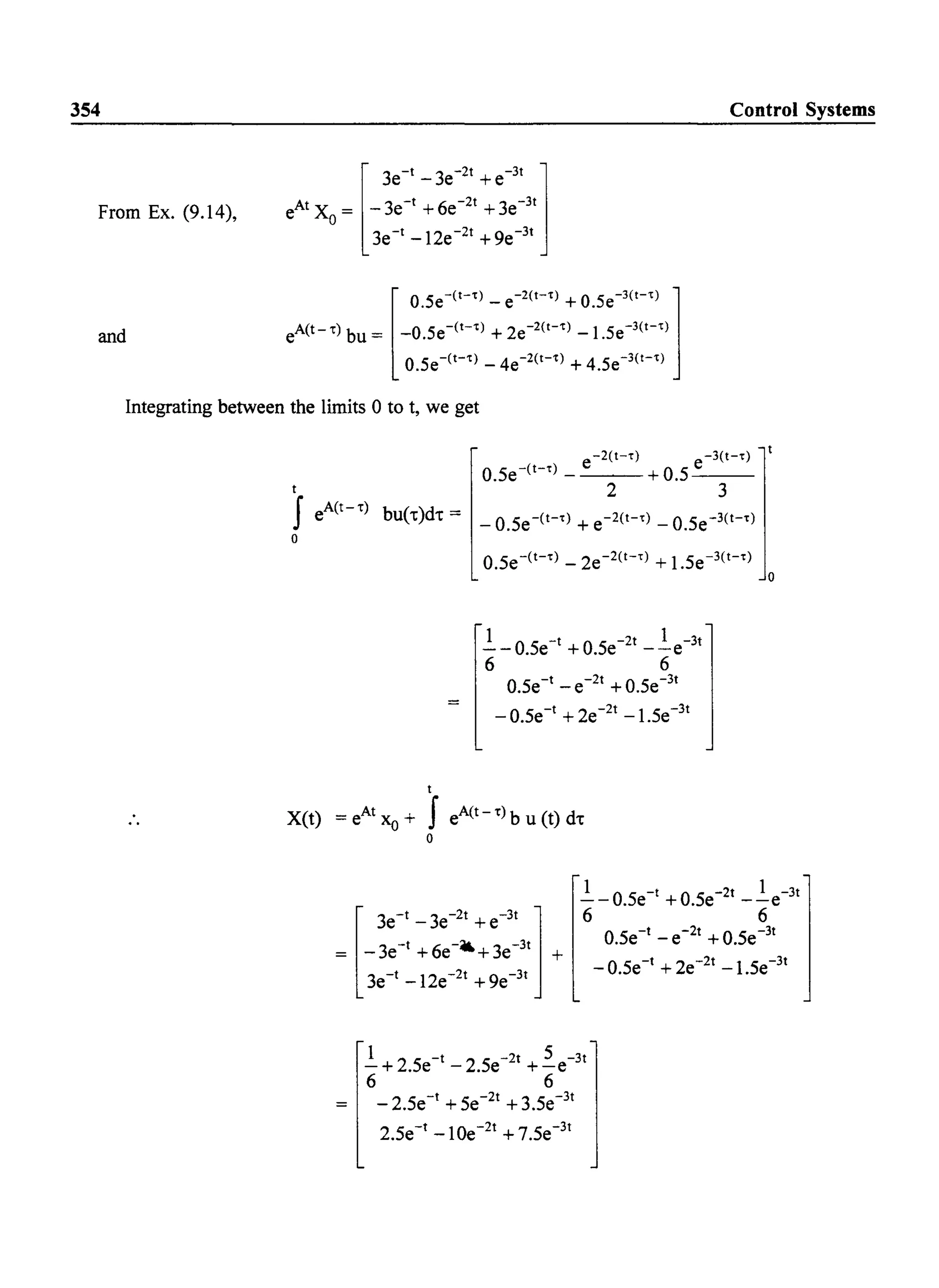
364. State Space Analysis of Control Systems
Example 9.18
Obtain the solution of the following state equation by first obtaining the canmical form.
With the initial condition X(O) = [1 0 - l]T
Solution:
355
First let us obtain the canmical form ofthe given state equation. The system matrix A is given by,
A = [~ ~ ~]
Let X=PZ
Where P is the modal matrix .
Modal matrix for this matrix A was obtained in Ex 9.9. Using the result, we have
[~
0
:]P= 1
0
[I 0-I]and p-1 = 0 1 -1
o 0 1
Using the transformation, we have
Z= p-l A P Z + p-l bu
(.: p-l AP gives the diagonal matrix with the eigen values 1,2 and 3 on the diagonal)
[
100] [-1]Z= ~ ~ ~ Z+ -~ U

365. 356
and Z(O) = p-l X (0)
Solution ofthe above equation is given by,
where
t
Z(t) = eJt Z(o) + feJ(t-t) bU('t)d't
a
Control Systems
The state transmition matrix eJt can be easily obtained since J is in diagonal form.
It is given by,
[e' 0
e;']e
Jt
= ~ e2t
0
Thus
[e' 0
e;'][~]+f~'
0
e"L][=:J dtZ (t) = ~ e2t e2(t-t)
0 0
nfe(H']Z (t) = 0 + t - e2
(t-t) d't
o a e3(t-t)

366. State Space Analysis of Control Systems
We have
e(t-t)
Z (t) = [~] +
e2(t-t)
2
_ e3(t-t)
3 0
Z (t) = m+ 2 2
1 e
3t
--+-
3 3
.!..(l-e2t )
2
..!..C-1+e3t)
3
XCt) = PZ Ct),
X(t) =
.!..(l_e2t )
2
..!..Ce3t -1)
3
e3t 2
-+-
3 3
1 1 2t 1 3t
---e +-e
6 2 3
..!..Ce
3t
-1)
3
357

367. 358 Control Systems
9.8 Qualitative Analysis of Control Systems
Sofar we have discussed,
(a) how to model a given physical system and
(b) solution of such a system for a given input, i.e., -quantitative analysis of the system.
We will now discuss some fundamental concepts about the control ofthese systems, i.e., qualitative
aspects of these systems, when a controller is to be designed to obtain a desired response.
There are two basic questions to be answered before we design a suitable controller for a given
system, namely,
(i) can we transfer the system from any initial state to any desired fmal state in fmite time by
applying a suitable unconstrained control.
(ii) by measuring the output for a finite length of time, can we determine the initial state of the
system.
These aspects were first introduced by Kalman and are defined as controllability and observability
of the system respectively. These aspects playa very important role in the design of a controller for
a given system. In this section we will only give elementary treatment of these aspects ofthe system.
9.B.l State Controllability
Definition
A system is said to be state controllable at t = to ifit is po~sible to transfer the initial state X (to) to any
final state X (tf) in fmite time, u&ing an unconstrained control signal u(t). Ifevery state is controllable,
the system is said to be completely state controllable.
Kalman's testfor control/ability
Consider the dynamical system described by the state equation,
X =AX+Bu
where X is a n-dimensional state vector
u is an scalar control signal
A is an n x n system matrix
B is an n x I input matrix
.....(9.118)
Without loss ofgenerality, let us consider the initial time 10 = 0 and the fmal desired state to be the
origin of the state space.
The solution of the state eqn. (9.118) is given by,
t
X(t) = eAtX(O) + f eA(t--c)B uCr) dt
o

368. State Space Analysis of Control Systems
Since the fmal state at t = tf Le., X(tf) = 0, we have,
t
f
or
X(tf) = 0 = eAtf X(O) + f eA(tf-t) B u(.) d.
o
tf
X(O) = _e-Atf f eA(tf-t) B u(.) d.
o
t
f
X(O) = - fe-At B u(.) d.
• 0
359
.....(9.119)
If we are able to obtain a u(t) for any given X(O) from eqn. (9.119), the system is controllable.
Using eqn. (9.116) with f(A) = e-At, we can write e-At as,
Substituting eqn. (9.120) in eqn. (9.119), we have,
Let·
Then
Eqn. (9.122) can be written in the matrix form,
~o
~I
X(O) = [B : AB : A2B : ..... : An-IB] ~2
.....(9.120)
.....(9.121)
.....(9.122)
.....(9.123)
A control u(t) exists, which transfers any given initial state X(O) to the origin of state space, ifthe
vector [~o' ~l' ... ~n- dT
can be obtained from eqn. (9.123). It requires that the n x n matrix
[B : AB : A2B : ... : An-IBJ
be non singular, i.e., its rank be equal to n.

369. 360 Control Systems
This result can be extended to a more general case where the input vector is ofdimension r. In the'
equation
u is an m-vector and
B is an n x m matrix
X =AX+Bu
The controllability condition in this case can be stated as :
The (n x nm) matrix
has a rank n.
.....(9.124)
.....(9.125)
The matrix Qc is known as the controllability matrix. For complete state controllability, therefore,
all the columns ofQc must be linearly independent. This test for deciding the controllability is known
as Kalman's test for controllability.
Gilbert's testfor Controllability
Let us now consider an alternate test for examining the controllability of a given system. Let us
suppose that the eigenvalues ofA in eqn. (9.124) are distinct. It is possible to transform the A matrix
into a diagonal matrix using a transformation matrix P. As already discussed in section 9.6, if
X=PZ
eqn. (9.124) can be transformed to
Z = p-l APZ + p-l Bu .....(9.126)
where P matrix is the modal matrix and p-l AP is a diagonal matrix with eigen values on the
diagonal. Eqns. (9.126) are first order uncoupled differential equations. The kth equation is given by
Zk = Ak ~ + akl ul + a k2 ~ + ... + akIn urn
where Ak is the kth eigenvalue ofA
and akl, a k2, ... akIn' are the kth row elements of p-l B
If all the elements ofkth row ofP-l B, i.e.,
akl = a k2 = ... = akIn = 0
.....(9.127)
then no control signal exists in eqn. (9.127) and hence the state variable Zk cannot be controlled.
Hence the condition for complete state controllability is that none of the rows of P-lB in
eqn. (9.126) should contain all zeros.
The above treatment can be extended to the case where the matrix A has repeated eigen values.
In this case the matrix A can be transformed to Jordon's cononical form. If P is the modal matrix
which transforms A into its Jordon form, let
and hence
X=PZ
Z =p-l APZ+p-l Bu
=JZ+p-1 Bu .....(9.128)

370. State Space Analysis of Control Systems 361
For a 7th
order system with eigen values AI' AI' A2, A2, A2, A3, and A4, J is of the form,
Al 1 1 0 0 0 0 0
o All 0 0 0 0 0
----+------,
0 o 1 A2 1 o 1 0 0
1
J= 0 0
1
1
0 A2 1 1
0 0 .....(9.129)
0 0 1 0 0 A2 1 0 0L _ _ _ _ _ _ +_,
0 0 0 0 o 1 A3 1 0L._r-,
0 0 0 0 0 o 1 A 1
• _4
Each square block is called a Jordon block, as discussed earlier. J can thus be written as,
where J1 is of order 2
J2 is of order 3
and J3, J4 are each of order 1
The condition for complete state controllability by this method can be stated as follows:
The system is completely state controllable if and only if,
1. No two Jordon blocks in eqn. (9.129), are associated with the same eigen value.
2. The elements of the row of p-l B corresponding to the last row of any Jordon block of J are
not all zero. If some of the Jordon blocks are of order 1, i.e., the corresponding eigen values
are distinct, the rows in p-l B corresponding to these eigen values must not contain all zeros.
It is to be noted that application of Gilbert's method requires that the equations be put in the
Jordon's form. Kalman's test can be applied to any representation of the given system.
Output Controllability
In practical systems, we may have to control the output rather than the states. In such cases, we can
define output controllability. State controllability is neither necessary nor sufficient for controlling the
output.
Consider the system
x - is an n vector
u - is an m vector
Y - is a p vector
X =AX+Bu
Y=CX+Du .....(9.130)

371. 362 Control Systems
The above system is completely output controllable if it is possible to find an unconstrained
control vector u(t) which will transfer any given initial output Y (to) to any final output Y (9 in fmite
time.
The test for complete controllability of the system in eqn. (9.130) is that the rank of the
[p x (n + 1) m] matrix,
.....(9.131)
be equal to p.
If in a particular system D = 0 i.e., the system output does not directly depend on the input, the
rank of the matrix,
must be p.
Example -9.19
Test the following systems for controllability using (i) Kalman's test (ii) Gilbert's test.
(a) A=[j -1~ JB=m
(c) A = [~ ~ ~l002
B= [i]
Solution:
(a) A=[j -1~ JB=m
(i) Kalman's test
The controllability matrix,
Qc=[B:AB:A2B]
[
0 0 II= 0 1-6
1 -6 25
The rank of Qc is 3.
Hence the system is controllable.
(b)
A= [~
(d) A= [~
0
2
0
2
0
~l B= Hl
~l B= Hl
.....(9.132)

372. State Space Analysis of Control Systems
(ii) Gilberts test
The eigen values are -I, -2,-3
The modal matrix P is given by,
[
3 2.5 0.5]
p-l = -3 -4 -1
1 1.5 0.5
p-l B = [-~ ~ ~~] [~]1 1.5 0.5 1
_ [0.5]- -1
0.5
363
Since all the eigenvalues are distinct and none of the elements of p-l B is zero, the system is
completely state controllable.
(b)
(i) Kalman's test
The controllability matrix,
The rank of this matrix is 2 and hence the system is not controllable.

373. 364 Control Systems
(ii) Gilbert's method
From example 9.9, we have the eigen values to be 1,2, and 3 and the modal matrix P to
be,
p =[~
0
:]1
0
[1 0-1]p-l = 0 1 -1
o 0 1
=[~
0
=:J [-:]and p-l B
0
=H]
Since the first element in p-1B is zero, the system is not controllable.
(i) Kalman's test
The controllability matrix,
Qc = [i ~ ~]
The rank of this matrix is 1 and hence the system is not controllable.
(ii) Gilbert's test
The eigen values are 1, 2 and 2.
From example 9.10, the modal matrix Pis
[
112]P = 0 1 1
o 0 1

374. State Space Analysis of Control Systems 365
and the Jordon form ofA is J ~ l~ ~ r]
~l~ l~
-1
-1]1 -1
0 1
= l~
-1
~:Hl]and p-I B 1
0
~m
Since the first element of p-I B corresponding to the distinct eigen value, Al = 1, is zero
and the last row element of p-I B corresponding to the repeated eigen value, ~ = 2, is
also zero the system is not controllable.
(d) A~l~ ~~] B~H]
(i) Kalman's test
The controllability matrix,
Qc = H-~ ~]
Since the rank of this is 1, the system is not controllable.
(ii) Gilbert's method
From example 9.11, the eigen values, the model matrix P, and its inverse are,
Al = 1, A2 = A3 = 1 ;
~ ~]; p-I = r~ ~1
-1 0 lo
-2]-1
2

375. 366 Control Systems
The Jordon fonn ofA is,
J ~p-l AP~ [~
0
~]2
0
~[~
0
nJ2
0
Since the Jordon block J2 and J3 are associated with the same eigen value 1..2 = 1..3 = 2,
the system is )1ot controllable. In this case, it is not necessary to fmd the elements of
P-lB. For any B, the system is not controllable.
Example 9.20
For the following system, detennine controllability.
[
2 0 0] [0 1]X = 0 2 0 X+ 1 0 [~l]
o 3 1 0 1 2
Solution:
The controllability matrix,
Qc = [B : AB : A2B]
The rank of this matrix is 3 and hence the system is completely state controllable.
9.8.2 Observability
Now let us define the second aspect of the system, i.e., observability.
Definition
A system is said to be completely observable, if every state X(to) can be detennined from the
measurement of the output Y(t) over a finite time interval, to ~ t ~ tf
.
This property ofthe system is very useful, because the state vector can be constructed by observing
the output variables over a finite interval of time. Therefore even if some states are not measurable,
they can be estimated using the measurable output variables over a finite time. Estimation of all the
state variables is required in some cases, when these state variables have to be fedback to obtain a
desired control.

376. State Space Analysis of Control Systems
Kalman's testfor observability
Consider the following system,
X =AX+Bu
Y=CX
The condition for complete state observability is that the observability matrix,
has a rank n.
C
CA
Qo= CA2
CAn- 1
Gilbert's testfor observability
367
.....(9.133)
.....(9.134)
The state equations represented by eqn. (9.133) can be transformed to its canonical form using the
transformation,
X=PZ
z= p-l APZ + p-l Bu
Y=CPZ
.....(9.135)
Since p-lAP is a diagonal matrix, the states are decoupled. Information about one state is not
available in the other state equations. Since Y is a combination of these decoupled states, if any
column ofCP in eqn. (9.135) is zero, the corresponding state variable does not affect the output Y,
i.e., if the jth column of CP contains all zeros, then the state variable ZJ is not observable from the
output. This is the condition if all eigen values ofA are distinct.
Ifsome ofthe eigen values are repeated, the matrix p-l AP is in Jordon form and the conditions for
complete state observability are stated as follows:
The system is completely state observable if,
I. no two Jordon blocks in J = p-l AP are associated with the same eigen value.
2. no columns of CP that correspond to the first row of each Jordon block consist of zero
elements. If some of the eigen values are distinct, the Jordon blocks corresponding to these
eigen values are of order I and hence the columns of CP corresponding to these block must
not be all zero.
The above conditions can be best illustrated by the following examples:
(a) [-2 0]X= 0 -4 X Y = [2 -2] X
The system is observable since C has no zero elements.

377. 368
(b)
(c)
(d)
(e)
Control Systems
. [-1 0]X = 0 -1 X Y=[l -l]X
Not observable since two Jordon blocks are associated with the same eigen value-1.
x= [-~ -~ ~] X
o 0-2
Y = [a b c] X
(i) If a = 0 and / or c :t:. 0 the system is not observable.
(ii) If a :t:. 0 and c:t:. O. the system is observable.
[
=-1~ ~ __0__ ~I
. 0 1 -2 1 0
X r- 0: 0 -2 1 X
1
o 1 0 0-2
Since all the elements of first column of C of Jordon block corresponding to the :!igenvalue
A= -1 are non zero and all the elements offirst column ofC ofthe Jordon block corresponding
to the repeated eigenvalue A= -2 are non zero, the system is completely observable.
1
-3 1 1 0 01
X = - ~ - ~3_ ~ ~- - ~ X
o 0 1-2 1
1
o 0 1 0 -2
[
0 1 1 2 -1]
Y=OO:O 1 X
Since all the elements of column 1 of C corresponding to the Jordon block of the repeated
eigenvalue A= -3 are zero, the system is not observable.
Problem 9.21
Comment on the complete state observability of the following systems using,
(i) Kalman's test
(ii) Gilbert's test
(a) x= [j 0
Jx-11
Y = [1 -1 1] X
= [~ I 2]X 2 1 X
o 2
(b) Y = [1 -1 0] X

378. State Space Analysis of Control Systems
(c) Y = [1 0 0] X
(b) Y=[~ 0~]X
Solution:
(a)
(b)
x = [~ ~ ~] X
-6 -11 -6
Y = [1 0 0] X
(i) Kalman's test
The observability matrix,
QO = [C~]= r~ 0~]CA2 0 0 1
The rank of Qo is 3 and hence the system is observable.
(ii) Gilbert's test
The model matrix for this system is,
p+: -~ -i]
CP = [I 0 0] [-: -~ -i]
= [1 1]
Since none of the columns of CP are zero, the system is completely observable.
[
1 1 2]X= 0 2 1 X
002
Y = [1 -1 0] X
369

379. 370 Control Systems
(c)
(i) Kalman's test
The observability matrix,
The rank of Qo is 2 and hence the system is not observable.
(ii) Gilbert's test
The modal matrix Pis,
The transformed equations are,
Y=CPZ
= [1 -1 0] [~ ~ ~l Z
o 0 1
= [1 0 1] Z
Since the first column of CP corresponding to the Jordon block of eigen value A= 2 is
zero, the system is not observable.
Y = [1 0 0] X
(i) Kalman's test
The observability matrix,
Qo= [~A 1=[~ ~ ~lCA2
1 3 6
Since the rank of Qo is 2, the system is not observable.

380. State Space Analysis of Control Systems 371
(d)
(ii) Gilbert's test
The modal matrix for the system is,
[
1 0 1]P = 0 2 1
o -1 0
The Jordon form of the system is
[
I'0 0]Z= Oi2~0 zL _ + _
o 0 ,2
[1_021 ~1]Y= [1 0 0] ~
= [1 0 0] Z
Since two Jordon blocks correspond to the same eigen value A= 2, the system is not
observable.
x=[~
0
~] X
Y= [~
0
~] X2
0
(i) Kalman's test
The observability matrix,
0 1
0 0
1 0 5
Qo =
0 2
1 0 17
0 4 5
The rank of Qo is 3 and hence the system is observable.
(ii) Gilbert's test
The modal matrix P and the Jordon form of the equations are,
[
101]P = 0 1 1
o 0 1

381. 372 Control Systems
Z~[~
0
~l z
and 2
0
Y= [~
0
~l [~
0
:Jz0
= [~ o 2]lIZ
Since none of the columns ofY contain all zero elements, and the eigenvalues ofA are
distinct, the system is observable.
9.8.3 Duality Principle
Kalman has introduced the duality principle to establish the relationship between controllability and
observability.
Consider system 1,
X =AX+Bu
Y=CX
and its dual defined by system 2,
Z=A* Z+C* V
W=B*Z
where A*, B* and C* are conjugate transpose ofA, B and C respectively.
The duality principle states that,
(i) if the pair (A, B) is controllable in system I, the pair (A*, B*) is observable in its dual
system 2.
and (ii) if the pair (A, C) is observable in system 1, the pair (A* C*) is controllable in its dual
system 2.

382. State Space Analysis of Control Systems 373
Problems
9.1 Obtain the state space representation of the electrical system shown in Fig. P 9.1.
2n
+
+
v IF
Fig. P.1
Take
v=u and
9.2 Obtain the state space representation for the mechanical system shown in Fig. P 9.2 taking
the displacement and velocity of the mass as state variables
B
x
Fig. P.2
9.3 The block diagram ofa position control system is shown in Fig. P 9.3. Obtain the state space
representation of the system.
Fig. P.3
Choose the state variables as

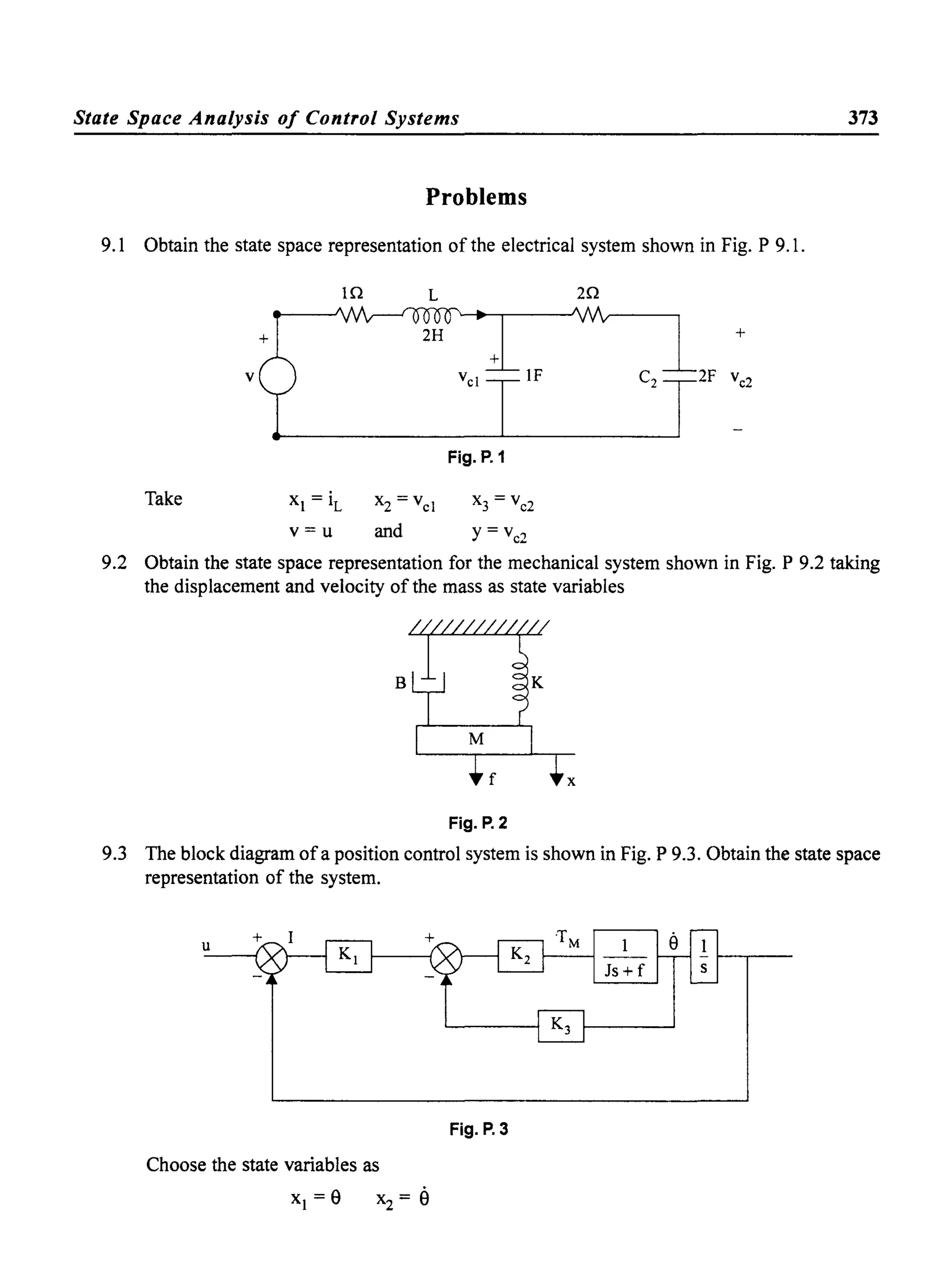
383. 374 Control Systems
9.4 Obtain the state space representation of the system shown in Fig. P 9.4.
Take c = xl' C = x2 and m = x3
u 10 m
s+4 S2 +s+1
Fig.P.4
9.5 Obtain the state space representation in,
(i) Companion form or Bush's form
(li) Diagonal/Jordon form
for the following systems.
(a) y + 9 x + 23 x + 15 = u
(b) Y+ 9 x + 23 x + 15 = ti - 2 U + 4u
9.6 Obtain the state space representation in,
(i) Phase variable form and
(ii) Jordon's form
for the systems whose transfer functions are given by,
s+1
(a) s(s + 4)(s +5)
(b) s+5
(s +1)2(S + 4)
9.7 Obtain the transfer functions of the following systems.
C(s)
(c)
10
(s +1)3
1. X = [~ ~ ~j X + [~j u
-2 -3 -4 1
2. X = [~ ~ ~j X + [~j u
-4 -6 -8 1
y = [1 0 0] X Y= [-2 4 0] X + 2u
3. X = n-~ JX+ [~j u
y = [-1 2 4] X

384. State Space Analysis of Control Systems
9.8 Find the transfer function of the systems given below.
2. X~[! -; ~]x+[_~]u
y = [1 0] X y = [1 1 -1] X
9.9 Transform the following matrices into Diagonal/Jordon form representations.
[
0 1
(i) A = 0 0
6 5
[
-2
(iii) A = - ~
(ii)
(iv)
(vi)
A= [~ ~ ~]-1 -3 -3
A= [-~ -~ ~]
1 -1 -2
-1 0]-2 0
o -1
9.10 Find the state transition matrix for the following systems.
(i) X= [~ ~] X (ii) X=[ 1 0 ] X
-1 -2
(iii) X=[~ ~ ~] X
-2 -5 -4
9.11 Obtain the solution ofthe state equation
X = [~ _~] X + [~] u
Xo = [1 l]T and u(t) is a unit step input.
375
9.12 Obtain the Jordon's cononical form ofthe following system and obtain its solution for a step
input
X = [~~ ~] X + [~] u
6 5 -2 1
X(o) = [1 0 O]T

385. 376 Control Systems
9.13 Determine whether the following systems are completely state controllable and observable
using (i) Kalman's test and (ii) Gilbert's test.
Y = [1 1 0] X
Y=[~ 0 ~]X
(e) X = [~ ~ _~] X{l Y=[O 1 -l]X
Jx+Hu(d) X = [~ ~
-1 -3
Y = [0 1 -1] X
9.14 Determine output controllability of system in problem P. 9.13 (b).
-djl-

386. Answers to Problems
Chapter 2
2.1
[
s(L-R2C) 1(a)
(LS +R)(RCS +1)
(b)
s(2s2
+ 2s + 1)
(2s4 + 14s3 + 232s + 20s + 8)
2.2 (a) K
MM2s4 + MB2s
3
+ (KM! + K2M + KM2)S2 + B2Ks + KK2
MS2
(b) MS2 + Bs+ K
(c)
K
2.3 T(s) = s(J S2 +B )
eq eq
_ (N4)2 (N4)2 (N2)2
Beq-BL +B2 N3 +Bl N3 N
2.5
Kf

387. 378
2.6
2.7
2.8
2.9
2.10
2.11
2.12
2.13
2.14
R
(i)
RCS+l
elm = -,:---------:;-
Y[Ls
2
+ ~S +1]g Ay
[RIR2CIC2S2 + (R2C2 + RICI + R IC2)S + 1]
10.87KA
S2 +54.35KKA +10.87KA
15
S2 +6.5s +15
Control Systems
GIG2G3 +G4
, ~= 1 +GI G2 HI +G2 G3 H2 +GI G2G3+G4-G4G2H2HI
~
1.
2.
3.
(a)
1+ G 2H 2 + G2G3H3 + G IG 2H 2 + GIG 2G3HI
GIG 2G 3(1+G4 )
G I(G2 + G3)(l-G4H 2)
I+GI(G2 +G3)HIH 2
PI = GI G2 G3 G4 Gs P2 = G I G2 G6 Gs
LI =-GI HI L2 =-GI G2
L3 =-G3H3 L4 =-G4 H4
Ls =-Gs Hs L6 =-GI G2 G3
L7=G6 H3H4
~ = 1 - (LI + L2 + L3 + L4 + Ls + L6 + L7) + LI L3 + LI L4 + LI Ls + L2 L4 + L2 Ls
+ L3 Ls + LI L7 - LI L3 Ls
~I = ~2 = 1
PI~I +P2~2
T = -'----=-------=---=-
~
(b) G IG 2G3G 4 (1 + G 7GgH2) + G 4G6G 7Gg(l + G 2G3HI) + GIG2G7GgG9
1+ G 2G3HI + G 7GsH2

388. Answers to Problems
2.15
4s3
+ 2S2 + 3s + 2
8s4
+ 17s3
+ 19s2+ ISs +6
2.17 (a) 60 V, 190V (b) 0.1
(c) 197.14V (d) 81.14V
2.18 S~ = 0.0125 S1 = 5.12 Si = 0.128
2.19 0.089
1.367
2.20
s(0.0118s+1)
Chapter 3
3.1 T(s) = S2 + 225.2s + 15KA
0=0.75
ron = 150 rad/sec
tp = 0.0317 s
~ = 2.84% ts = 0.0356 sec
3.2 (i) Mp = 10.07% ~ = 0.6s ts = 1.043 s
(ii) KA =7
(iii) KA = 23.64
3.3 T = 1.44 sec
3.4 (i) ron = 3.16 rad/sec
(ii) 0.1792
K = 1.06
0=0.316
3.5 (i) 0 = 0.316
(ii) Kr= 1.212
(iii) ~ = 2.6
3.6 K = 2.95
3.7 K= 16
3.8
1
(i) 0, 3"' 00
(iii) 0, 0, 0.01
COn = 3.16 rad/sec
ess = 0.4424 rad
KA = 18
a = 0.47 sec
a = 0.175
..) 1
(11 11' 00, 00,
(iv) 0, 0.1, 00,
9css = 0.2 rad
c(t) = 1 - 1.25 e-2
.4t sin (3.2t + 53.13°)
379

389. 380 Control Systems
3.9 K=23 a=0.163
3.10 esit) = 0.54625 + 1.075t + 0.75r
3.11 (a) ess(t) = O.Olt + 0.0009 (b) ess<t) = O.Olt + 0.0209
Chapter 4
4.1 (a) al' 8,z, > 0
(b) ai' 8,z, a3, > 0 ai' 8,z, > a3
(c) ai' ~, a3, a4, > 0 al 8,z, > a3, a4 < a3
(al a2 - a3)
a 2
I
4.2 (a) -2.5 ±j2.784
(b) -2, -2
(c) -1, -3, --6
4.3 (a) 1±j1,-1±j1
(b) -4.495, 0.2475 ± j1.471
(c) 0.1789, -11.179
4.4 (a) Stable
(b) Stable
(c) Two poles in RHS
(d) Four roots on jro-axis
(e) Two roots in RHS
4.5 (a) k> 0.303
(b) No real value ofk
(c) > 1
4.6 0< k < 99
4.7 (a) equal
(b) less
(c) greater
4.8 -1 ±j2; -2 ±j1

390. Answers to Problems
Chapter 5
5.1 (i) (a) -5 (b) 60, 180, -60 (c) -1.79 (d) K = 660 (e) 0) = 8.63 rad/sec
(ii) (a) -7 (b) 90, -90 (c) -7.37
(iii) (a) -1 (b) +60, 180, -60 (d) 48.6° (e) K = 8, 0) = 2 rad/sec
(iv) (b) 180° (c) 0.414, -2.414 (e) K = 1,0) = 1.225 rad/sec
5.2 K = 19.05 0 = 0.189, O)d = 2.6 rad/sec ts = 7.986 sec
Closed loop poles for K = 19.05: -5, -0.5 ±j 2.6
5.3 K = 2.96
5.4 -5.52, -43.8°, -2.5
5.5 1. Stable for K < 30 ; root locus bends towards RHP
2. Stable for K < 70.68 ; bends towars RHP
5.6 (i) Root locus bends towards LHP, breakaway point moves to the left.
Original system is stable for K < 42, Modified system is stable for K > 0
(ii) System is stable for all positive values of K
5.7 K=4 s=-I±j1,-3±jl
K = 64 O)n = 2 rad/sec
5.8 (a) -385,60°, 180°, -60°
(b) 60°, -60°
(c) Kl = 1.1 x 106
, 0)1 = 16.6 rad/sec
5.10 Root locus bends towards LHP
Stable for K < 22.75
Chapter 6
6.1 (i) Mr = 1.04 O)r = 2.116 rad/sec
(ii) Mr= 1.0 O)r = 0
(iii) ~= 1.0 O)r = 0
(iv) Mr = 1.364 O)r = 6.6 rad/sec
O)b = 4.592 rad/sec
O)b = 4 rad/sec
O)b = 8.7 rad/sec
O)b = 11 rad/sec
381

391. 382
6.2 (i) 4.1 rad/sec
(ii) 0.75 rad/sec
6.3 (i) K=200
(ii) K=398
6.4 (a)
10(0.5s +1)
s(0.02s +1)
O.4s
(b)
(0.2s +1)(0.05s +1)(0.005s +1)
6.5
10(s + 2)
s(s +l)(s +10)
6.6 K= 14.91
~ = 14.62
6.7 ~= 1.5
Poles = -2.11 ±j5.53
6.8 (a) Does not cross
(b) ro = 2.236 rad/sec,
(c) ro = 4.795 rad/sec,
(d) ro = 37.42 rad/sec,
6.9 ro = 0.2 rad/sec
Chapter 7
7.1 (a) 2 roots in RHP
(b) 2 roots on jro-axis
(c) 2 roots in RHP
't = 0.0616 s
ts = 0.4924 s
ror = 5.1 rad/sec
IGI = 0.077
IGI = 0.11
IGI = 2.38 x 10-3
jGGro) = 93.44°
Control Systems
7.2 At ro = 0 and ro = 00 the curve is rotated by 90° in clockwise direction for addition of every
pole at origin.
7.3 The behaviour at ro = 0 is not altered but at ro = 00, the curve is rotated by 90° in clockwise
direction for every non zero pole added.

392. Answers to Problems
7.4 1m
GH-plane
Re
7.5 (a) (b)
7.7 K = 0.7, The system becomes more stable, K = 1.08
7.8
7.9
7.10
(a) Unstable
GM = 9.54db 4>pm = 32.6°
(a) GM = 28 db .h = 76°'l'pm
(b) K = 4.45
(c) K=4.33
7.12 ~ = 1.78 ror = 8 rad/sec
Chapter 8
8.1 (i) 4> = 40°pm
(li) roge = 0.5 rad/sec
(iii) eff =0.2
(iv) Gain margin = 11 db
(b) Stable
rob = 10 rad/sec
383

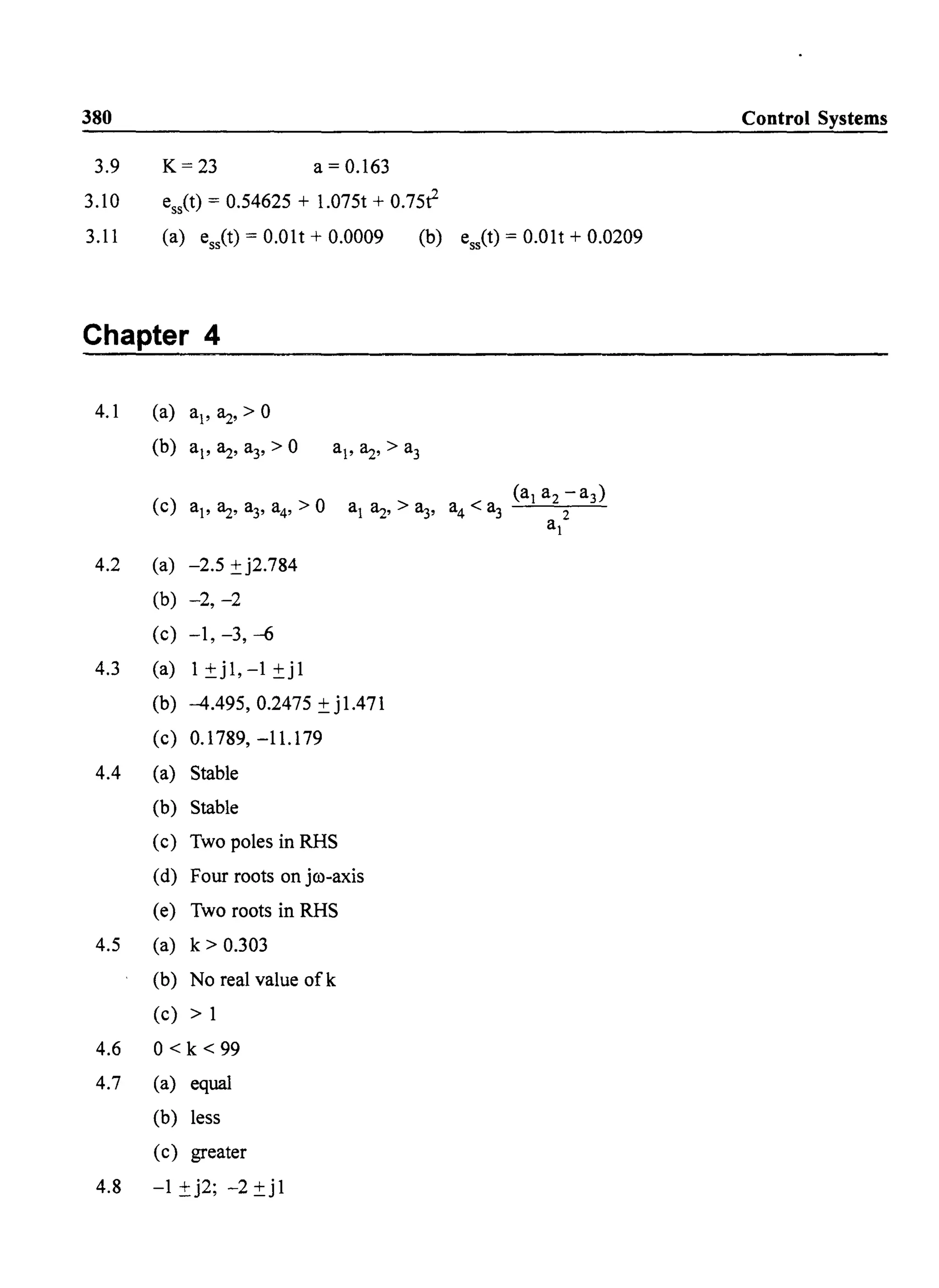
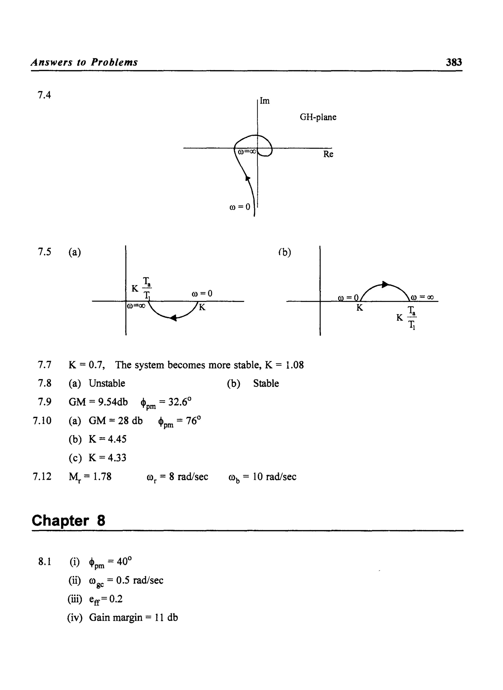
393. 384 Control Systems
Chapter 9
1 1
0-- --
2 2 -
1 1
2
9.1 x= -- - x+ 0 u
2 2
y = [0 0 1] X
0
1 1 0- --
4 4
9.2
x=l-: d x+ [~lu
9.3 x=[-K;OK, -[f)'JK3] X+ [Kl;}
9.4 x=[-~ -~ ~] x+ [~] u Y=[1 0 O]X
-10 0 -4 10
9.5 (a) (i) A = [~ ~ ~l B = [~] C = [1 1 0]
-15 -23 -9 1
(ti) A=[-~ -~ _~] B=[:] c=[i ~ iJ
(b) (i) A = [~ ~ ~] B = [~] C = [4 -2 1]
-15 -23 -9 1
(ii) A = [-~ - ~~] B = [~] C = [i -~9
3:]o 0 -5 1

394. Answers to Problems 385
9.6 (a) (i)
A~[~ 0
~;J B=[~! c = [1 1 0]
-20
A= [~
0
J B~[:1(ii) -4
C = [2
1
0
3
-54]-
0
4
(b) (i) A~[ ~ 0
J B=m C = [0 1 0]
-2 -5
[~I
~~J B=[:](ii) A= ~ -1 C= [j -1
~]-
0
9
(c) (i)
A= [ ~ 0
J B=m
C = [10 0 0]
-1 -3
[~I
J B~m(ii) A= ~ -1 C = [10 0 0]
0
2s3+16s2 +16s+6 3s2 +10s+6
9.7 1.
S3 +4S2 +3s+2
2.
S3 +8s2+6s+4
3.
(s + 1)(s + 2i
9.8 (i)
s-6
s(s - 5)
fii)
2
s+1

395. 386
9.9 (i) D= r-~ ~ ~]o 0 -3
(ii) J = r-~ -1 ~]o 0-1
9.10
9.11
9.12
9.13
9.14
(ill) r~ -1 _~] (iv) r-~ -1 ~lo 0 -2J
r
-1
0 001
(v) A= 00 -01
-2J r
-1 1 0](vi) A = 0 -1 0
o 0-1
(i)
(ii)
[ e'
tet ~,l
[(1+t)e-'
-te-t
te-
t
1(1- t)e-t
2e-2t -2e-t +3te-t
_4e-2t +5e-t -3te-t
8e-2t -8e-t +3te-t
-1 7 -t 7 2t 1 - 3t
-+-e +-e +-e
6 6 30 6
-7 -t 7 2t 1 -3t
-e +-e --e
6 15 2
X(t) =
(a)
(b)
(c)
(d)
7 -t 14 2t 3 -3t
-e +-e +-e
6 15 2
not controllable, not observable
controllable, not observable
not controllable, observable
controllable, observable
Output controllable
-jJ-
Control Systems

396. Multiple Choice Questions (MCQs) from
Competitive Examinations

397. 388 MCQs from Competitive Examinations
Chapter 1
1. Which one ofthe following is open loop?
(a) The respiratory system of man
(b) A system for controlling the movement ofthe slide of a copying milling machine
(c) A thermostatic control
(d) Traffic light control
2. Consider the following statements regarding a linear system y = f(x) :
1. f (xl + x2) = f (Xl) + f (x2).
2. f [x(t + T)] = f [x(t)] + f [x(T)].
3. f (Kx) = Kf (x).
Of these statements
(a) 1, 2 and 3 are correct
(c) 3 alone is correct
(b) 1 and 2 are correct
(d) 1 and 3 are correct.
3. Which one ofthe following is an example of open-loop system?
(a) A windscreen wiper
(b) Aqualung
(c) Respiratory system of an animal
(d) A system for controlling Anti-rocket-missiles
4. When a human being tries to approach an object, his brain acts as
(a) an error measuring device (b) a controller
(c) an actuator (d) anamplifier
5. In a continuous data system
(a) data may be a continuous function of time at all points in the system
(b) data is necessarily a continuous function oftime at all points in the system
(c) data is continuous at the input and output parts of the system but not necessarily
during intermediate processing of the data.
(d) Only the reference signal is a continuous function of time.
6. As compared to a closed-loop system, an open-loop system is
(a) more stable as well as more accurate
(b) less stable as well as less accurate
(c) more stable but less accurate
(d) less stable but more accurate
7. The principles ofhomogeneity and superposition are applied to
(a) linear time variant systems (b) non-linear time variant systems
(c) linear time invariant systems (d) non-linear time invariant systems

398. MCQs from Competitive Examinations 389
Chapter 2
1. For block diagram shown in Fig. C(s)/R(s) is given by
2.
(b)
G, G2 G3 +
l+G, G2 G3 H, H2 R(s) C(s)
(c)
G, G2G3
l+G, G2 G3H, +G, G2G3 H2
(d)
G, G2 G3
l+G, G2G3H,
d2
y dy du
The transfer function of the system described by dt2 + dt = dt + 2u with 'u' as input
and 'y' as output is
(a) (s+2)
(S2 +s)
(s + 1)
(b) (S2 +s)
2
(c)
(S2 + s)
3. Feedback control systems are
(a) Insensitive to both forward-and feedback-path parameter changes
(b) Less sensitive to feedback-path parameter changes than to forward-path parameter
changes
(c) less sensitive to forward-path parameter changes than to feedback-path parameter
changes.
(d) equally sensitive to forward and feedback-path parameter changes.
4. A system is represented by the block diagram given in the figure.
Which one ofthe following represents the input-output relationship ofthe above diagram
(a) R(s) ~1(GIG2)1~ C(s)
(b) R(s) ~I(GI + G2)1~ C(s)
(c) R(s) ~ 11 + G1 + GIG21~ C(s)
(d) R(s) ~Il + G2+ GIG21~ C(s)
R(s) C(s)
1~

399. 390 MCQs from Competitive Examinations
5. Consider a simple mass-spring-friction system as given in the figure.
6.
7.
KI , ~ - Spring Constants, f - Friction
M - Mass, F - Force, x - Displacement
The transfer function Xes) of the given system will be
F(s)
(a)
MS2 +fs+K,.K2
(b)
MS2 +fs+K, +K2
(c) (d)
K2
MS2 +fs+ K,.K2 MS2+fs+K,
K, +K2
10
In the following block diagram, GI = 10/s, G2 = (s + 1) , HI = S + 3 and H2 = 1. The
overall transfer function CIR is given by
(a)
10
11s2 +31s+10
C
100
(b)
11s2 +31s+100
100 H2
(c)
11s2 + 31s + 10
100
(d)
11s2 + 31s
The signal flow of a system is shown in the given figure. In this graph, the number of
three non-touching loops is
(c) 2 (d) 3
R(s) ...---+@--...-~tt----t--+-_-e.C(s)
(a) zero (b)

400. MCQs from Competitive Examinations 391
8.
9.
10.
11.
The sum of products of two non-touching loops in the following signal flow graph is
(a) S3 t32 t44 t44
(b) S3 t32 + t34 t43
t12 1
xl l<t;
(c) S3 t32 + t34 t43 + t44 ":2 Xs
(d) S4 t43 t32 + t44
t25
The closed-loop gain of the system in the given figure is
9 6
R(,)1
:J
C(s)
(a) (b) -
5 5
6 9
(c)
5
(d)
5
The response CCt) of a system to an input ret) is given by the following differential
. d2CCt) dCCt)
equatIOn: --+3-- + 5CCt) = 5 ret)
dt2 dt
The transfer function of the system is given by
5
(a) G(s) =
S2 +3s+5
(b) G(s) =
s2+3s+5
3s s+3
(c) G(s) =
S2 +3s+5
(d)
S2 +3s+5
For the RC circuit shown in the given figure, Vi and Vo are the input and output ofthe
system respectively. The block diagram of the system is represented by
R
r-;'VWvc I
~ I
System
v~
VoCs) V
L
Vo(s)
• •
(a) (b)
~
Vo(s)
V~
VO<s)
I
•
I
•llR cs
(c)
Vj(s) -
(d)

401. 392 MCQs from Competitive Examinations
12. Given : ~ = 99; s =j 1 rad/s, the sensitivity of the closed-loop system (shown in the
given figure) to variatiQ11 in parameter K is approximately
(a) 0.01 (b) 0.1 Er (s) KI(lOs + 1)
0
•
q • ow(s)
(c) 1.0 (d) 10 1 1
13. The transfer function CIR of the system shown in the figure is :
(a)
GI G2 H2
HI(I+GI G2 H2)
GI H2 R
(b)
HI(I+GI G2 HJ C
(c)
G2 H2
HI(I+GI G2 HJ G2
(d)
G2 HI
H2(I+GI G2 H2)
14. Laplace transform of the output response of a linear system is the system transfer
function when the input is
(a) a step signal (b) a ramp signal
(c) an inpulse signal (d) a sinusoidal signal
15. A simple electric water heater is shown in the given figure. The system can be modelled
by
Air at TOAC
Insulation
Water out
Heater
(a) a first order differential equation (b) a second order differential equation
(c) a third order differential equation (d) an algebraic equation

402. MCQs from Competitive Examinations 393
16. Which of the following is used in digital position control systems
(a) Stepper motor (b) AC servo motor
(c) Synchro Cd) DC servo motOl
17. Four speed-torque curves (labelled I, II, III and IV) are shown in the given figure. That
of an ac servomotor will be as in the curve tabelled
Torque
(a)
(b) II
(c) III
(d) N Speed
18. Match List I with List II and select the correct answer using the codes given below the
lists.
List I List II
A. Hydraulic actuator 1. Linear device
B. Flapper valve 2. AC servo systems
C. Potentiometer error detector 3. Large power to weight ratio
D. Dumb bell rotor 4. Pneumatic systems
Codes:
A B C D
(a) 4 3 2
(b) 3 4 2
(c) 3 4 2
Cd) 4 3 1 2
19. When the signal flow graph is as shown in the figure, the overall transfer function ofthe
systems, will be
C
(a) - =G
Q-Hl y-H2
R
G
C G •(b) - = - - R C
R 1+H2
(c)
C G
(d)
C G
R = (1+H1Xl+H2)
=
R l+Hl +H2

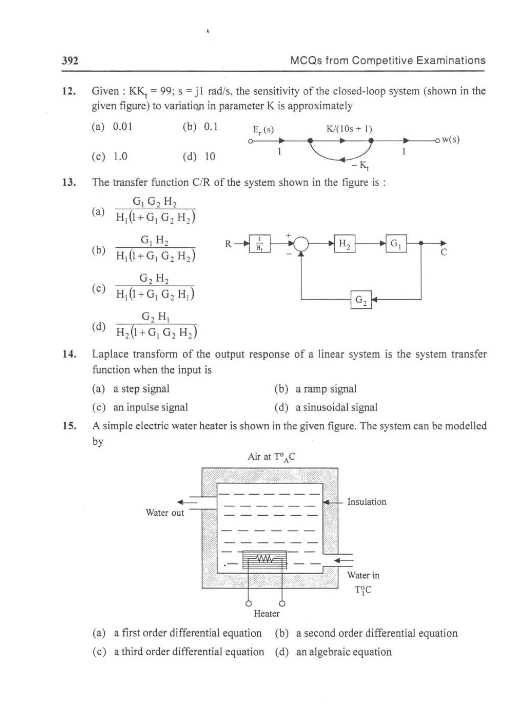
403. 394 MCQs from Competitive Examinations
20. The block diagram shown in Fig. 1 is equivalent to
Xl 0 ~
~
~C
x2
~C
'X2~
[QJ ~C
(a) (b)
x2
X2~
[QJ ~C Xl C
(c) (d)
x2
21. Consider the system shown in figure-I and figure-II. Ifthe forward path gain is reduced
by 10% in each system, then the variation in C1 and C2 will be respectively
(a) 10% and 10% cl
(b) 2% and 10%
Figure I
'r .. C2
I
(c) 5% and 1%
(d) 10% and 1% Figure II
22. The block diagrams shown in figure-I and figure-II are equivalent if 'X' (in figure-II) is
equal to
(a) 1
R(s)
(b) 2
R(s)
{lli] C(s)
(c) s + 1
..
s+l
C(s)
(d) s+2
23. The signal flow graph shown in the given figure has
(a) three forward paths and two non-touching loops C
(b) three forward paths and two loops R
(c) two forward paths and two non-touching loops
(b) two forward paths and three loops

404. MCQs from Competitive Examinations 395
24. In the system shown in the given figure, to eliminate the effect of disturbance D(s) on
C(s), the transfer function Gd (s) should be
(s +10)
(a) 10
10
(c)
s + 10
(b) s(s + 10)
10
10
(d) s(s+10)
25. Match List-I (Component) with List-II (Transfer functions) and select the correct answer
using the codes given below the lists :
26.
R(s)
•
List-J List-II
A. ac servo motor 1.
K
s(l + s 'tm)
B. Field controlled dc servo motor 2.
K
s(1 + s 'te)(l +s 'tm)
C. Tacho generator 3. Ks
K
1+ S't
D. Integrating gyro 4.
Codes:
(a) A B C D (b) A B C D
1 2 3 4 1 2 4 3
(c) A B C D (d) A B C D
2 3 4 2 4 3
A closed-loop system is shown in the given figure. The noise transfer function Cn (s)
N(s)
[Cn (s) = output corresponding to noise input N(s)] is approximately
1
(a) G(s)HJ(s) for IGI (s) HI (s) H2 (s)I« 1
1
(b) - - - for IGI (s) HI (s) ~ (s)1 » 1
HJ(s)
(c) - HJ(s)H2(S) for IGI (s) HI (s) H2 (s)I» 1
1
(d) G(s)HJ (S)H2(S) for IGI (s) HI (s) H2 (s)I« 1

405. 396 MCQs from Competitive Examinations
27. A signal flow graph is shown in the given figure. The number of forward paths M and
the number of individual loops P for this signal flow graph would be
(a) M = 4 and P = 3
(b) M = 6 and P= 3
(c) M = 4 and P = 6
(d) M=6andP=6
ret)
28. The mechanical system is shown in the given figure
The system is described as
(a) M d
2
Yl (t) + B dYI (t) = k[ (t) - (t)]
dt2 dt Y2 YI
(b) M d
2
Y2(t) + B dY2(t) = k[y (t) - y (t)]
dt2 dt 2 I
(c) M d
2
Yl(t) + B = k[YI(t) - Y2(t)]
dt2
(d) M d
2
Y2(t) + B dY2(t) = k[y (t) - Y (t)J
dt2 dt I 2
29. A synchro transmitter consists of a
c(t)
(a) salient pole rotor winding excited by an ac supply and a three-phase balanced stator
winding
(b) three-phase balanced stator winding excited by a three-phase balanced ac signal
and rotor connected to a dc voltage source
(c) salient pole rotor winding excited by a dc signal
(d) cylindrical rotor winding and a stepped stator excited by pulses
30. The torque-speed characteristic of two-phase induction motor is largely affected by
(a) voltage
R
(b) - and speed
X
X
(c) R (d) supply voltage frequency

406. MCQs from Competitive Examinations 397
31. Consider the following statements regarding A.C. servometer :
1. The torque-speed curve has negative slope.
2. It is sensitive to noise.
3. The rotor has high resistance and low inertia
4. It has slow acceleration.
Which of the following are the characteristic ofA.C. servomotor as control component?
(a) 1 and 2 (b) 2 and 3 (c) 1 and 3 (d) 2and4
32. Which of the following are the characteristics of closed-loop systems?
1. It does not compensate for disturbances.
2. It reduces the sensitivity of plant-parameter variations.
3. It does not involve output measurements.
4. It has the ability to control the system transient response.
Select the correct answer using the codes given below:
(a) 1 and 4 (b) 2 and 4 (c) 1 and 3 (d) 2 and 3
33. The number of forward paths and the number of non-touching loop pairs for the signal
flow graph given in the figure are, respectively,
(a) 1, 3 b
(b) 3, 2
(c) 3, 1
(d) 2,4
R(s) a
h
34. From the signal flow graph shown in the figure, the value of x6 is :
(a) de (ax + bX2 + cx3) XI
(b) (a + b + c) (x + x2 + x3) (d + e)
(c) (ax + bX2 + cx3) (d + e)
(d) abcde (x + x2 + x3)
g
d
35. From the figure shown, the transfer function of the signal flow graph is
(a) ~ (b) ~
1- T22 I-TI2
XI Tl2
0 •
(c) ~ (d)
T22
1+ T22 1+T12
C(s)
e
T22
CJ
x2

407. 398 MCQs from Competitive Examinations
36. A stepper motor
(a) is a two phase induction motor
(b) is a kind of rotating amplifier
(c) is an electromagnetic transducer commonly used to convert an angular position of
a shaft into an electrical system
(d) is an electromechanical device which-actuates a train of step angular (or linear)
movements in response to a train of input pulses on one to one basis.
37. Match List-I with List-II and select the correct answer by using the codes given below
the lists:
38.
39.
40.
41.
Codes:
(a) A
1
(c) A
3
A.
B.
C.
D.
B
2
B
2
List-I
Synchro
Amplidyne
Servo
RC Network
C
3
C
4
D
4
D
l.
2.
3.
4.
(b) A
4
(d) A
4
List-II
Amplifier
Actuator
Compensator
Transducer
B
3
B
C
2
C
2
D
1
D
3
The open-loop transfer function ofa unity feedback control system is G(s) = - - - ; 0 -
(s + 2)2
The closed-loop transfer function will have poles at
(a) -2, -2 (b) -2, -1 (c) -2 ±jl (d) -2,2
The signal flow diagram of a system is shown in the given figure. The number of
forward paths and the number of pairs of non-touching loops are respectively
(a) 3, 1
(b) 3,2
(c) 4,2
(d) 2,4
The ac motor used in servo applications is a
6
E
9
(a) single-phase induction motor (b) two-phase indl,lction motor
(c) three-phase induction motor (d) synchronous motor
A synchro transmitter-receiver unit is a
(a) two-phase ac device
(c) dc device
(b) 3-phase ac deVIce
(d) single-phase ac voltage device

408. MCQs from Competitive Examinations 399
42. Match the control system components in List-I with their functions in List-II and select
the correct answer using the codes given below the lists :
List-I List-II
A. Servo motor 1. Error detector
B. AmpJidyne 2. Transducer
C. Potentiometer 3. Actuator
D. Flapper valve 4. Power amplifier
Codes:
(a) A B C D (b) A B C D
3 1 2 4 3 4 2
(c) A B C D (d) A B C D
4 3 2 3 4 2
43. An electromechanical device which actuates a train ofstep angular movements in response
to a train of input pulses on one to one basis is
(a) synchro control transformer (b) LVDT
(c) stepper motor (d) ac tachogenerator
44. For a two-phase servo motor which one of the following statements is not true?
(a) The rotor diameter is small
(b) The rotor resistance is low
(c) The applied voltages are seldom balanced
(d) The torque speed characteristics are linear
45. Which one ofthe following transducers is used to obtain the output position in a position
control system?
(a) Strain Gauge (b) Loadcell (c) Synchro (d) Thermistor
46. For the system shown in the given figure the transfer function X(s) is
F(s)
1
(a) Ms2 +K (b)
1"x(t)
(c)
Ms2 +1
K
(d)
47. In case of synchro error detector, the electrical zero position of control-transformer is
obtained when angular displacement between rotors is
(a) zero (b) 45° (c) 90° (d) 180°

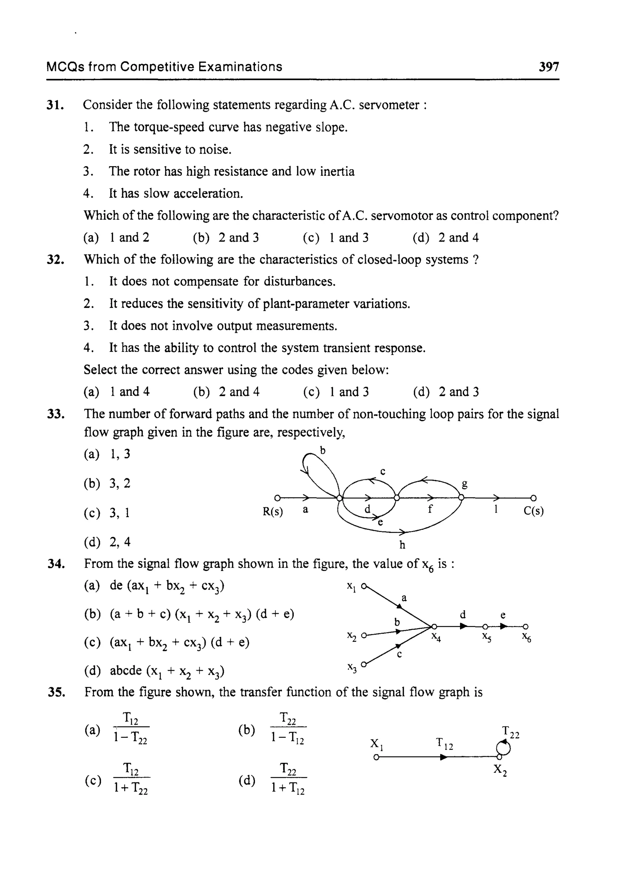
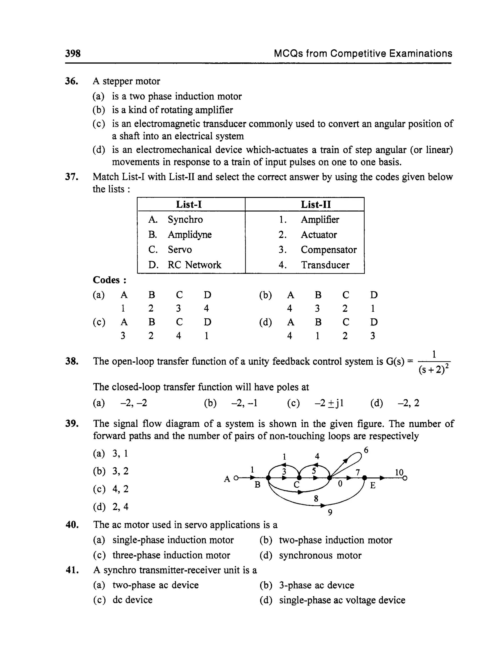
409. 400 MCQs from Competitive Examinations
48. The transfer function T(s) of the system shown in the following figure is given by
(a) T (s) = GI(S)G2(s)
1-G2(s)
b T (s) - GI (s)
( ) - 1-GI(s)G2
(s)
(c) T (s) = Gz(s)
1-GI(s)G2(s)
(d) T (s) = G2 (s)
1+GI(s)G2 (s)
C(s)
C(s)
T(s) = - -
R(s)
49. In a two-phase ac servometer, the rotor has a resistance R and a reactance X. The
torque-speed characteristic of the servomotor will be linear provided that
50.
51.
52.
X
(a) -« 1
R
X
(b) -» 1
R
x(c) - = 1
R
The C(s) for the system shown in the following block diagram is
R(s)
(a)
GI(s) Gz(s)
1+ GI(s)[G2 (s) + HI (s)]
R(s)
(b)
GI(S)G2 (s)
1+ G2 (s)[GI(s) + HI (s)]
(c)
GI(s)+GZ(s)
1+ G2 (s)[Gz(s) + HI (s)]
(d) none of the above
Which of the following can work as error detecting devices?
1. A pair ofpotentiometers 2. A pair of synchros
3. Ametadyne 4. A control transformer
Select the correct answer using the codes given below:
Codes:
(a) 1,2
(c) 1,3. 4
(b) 2,3, 4
(d) 1,2,4
G
The sensitivity SGM of a system with the transfer function M = - - is given by
l+GH
1
(a) 1+GH
l+GH
(b) H
l+G
(c) H (d) H

410. MCQs from Competitive Examinations 401
53. The signal graph ofa closed-loop system is shown in the figure, wherein TD represents
the distrubanct: in the forward path :
The effect of the disturbance can be reduced by
(a) increasing G2 (s)
(b) decreasing G2 (s)
(c) increasing G1 (s)
(d) decreasing G1 (s)
R(s)
-H(s)
54. Which is the following relate to rational transfer function of a system?
1. Ratio of Fourier transform of output to input with zero initial conditions
2. Ratio of Laplace transform ofoutput to input with zero initial conditions
3. Laplace transform of system impulse response
4. Laplace transform of system unit step response
Select the correct answer using the codes given below codes:
(a) 1and4 (b) 2and3 (c) 1and3 (d) 2and4
C(s)
55. The closed-loop system shown in the figure is subjected to a disturbance N(s). The
transfer function C(s) is given by
N(s)
(a)
GJ(s)G2 (s)
l+GJ(s)G2 (s)H(s)
(b)
GJ(s)
l+GJ(s)H(s)
(c)
G2 (s)
1-G2 (s)H(s)GJ(s) H(s)
(d)
G2 (s)
l+GJ(s)G2 (s)H(s)
56. Which of the following components can be used as a rotating amplifier in a control
system?
1. An amplidyne 2. A separatively excited dc generator
3. A self-excited dc generator 4. A synchro.
Select the correct answer using the codes given below
Codes:
(a) 3 and 4 (b) 1 and 2 (c) 1,2and3 (d) 1,2,3and4

411. 402 MCQs from Competitive Examinations
57. The transfer function of the system shown in the given figure is :
ABC
(a) 0 I R = 1+ ABC
A+B+C
(b) O/R= - - - -
l+AB+AC
AB+AC
(c) O/R= - - -
ABC
AB+AC
(d) O/R= - - - -
I+AB+AC
58. A signal flow graph is shown in the following figure:
Consider the following statements regarding the signal flow graph :
1. There are three forward paths.
2. There are three individual loops.
3. There are three sets of two non-touching loops.
Of these statements
(a) 1, 2, and 3 are correct
(b) 1 and 2 are correct bI
xl
"2
(c) 2 and 3 are correct
(d) 1 and 3 are correct
59. In the field-controlled motor, the entire damping comes from
(a) the armature resistance (b) the back emf
(c) the motor friction and load (d) field resistance
I---T-.O
60. Which of the following rotors are used in a two-phase ac servomotor?
1. Solid iron motor 2. Squirrel cage rotor 3. Drag cup rotor
Select the correct answer using the codes given below.
Codes:
(a) 1, 2 and 3 (b) 1 and 2 (c) 2and3 (d) 1 and 3
61. For two phase a.c. servomotor, if the rotor's resistance and reactance are respectively
R and X, its length and diameter are respectively Land D, then
(a) X and ~ are both small
R D
(b) X is large but ~ is small
R D
(c) X is small but ~ is large
R D
X L
(d) - and - are both large
R D

412. MCQs from Competitive Examinations 403
62. Consider the following statements relating to synchros :
1. The rotor of the control transformer is either disc shaped or umbrella shaped.
2. The rotor of the transmitter is so constructed as to have a low magnetic reluctance.
3. Transmitter and control transformer pair is used as an error detector.
Which of these statemens are correct ?
(a) 1,2 and 3 (b) 1 and 2 (c) 2 and 3 (d) 1 and 3
63. Consider the following servomotors:
1. a.c. two-phase servomotor 2. d.c. servomotor
3. Hydraulic servomotor 4. Pneumatic servomotor
The motor which has highest power handling capacity is
(a) 2 (b) 1 (c) 3 (d) 4
64. Match List I (Functional components) with List II (Devices) and select the correct
answer using the codes given below the Lists :
List I List II
A. Error detector 1. Three-phase FHP induction motor
B. Servomotor 2. A pair of synchronous transmitter and
control transformer
C. Amplifier 3. Tachogenerator
D. Feedback 4. Armature controlled FHP d.c. motor
5. AmpJidyne
Codes:
(a) A B C D
2 4 1 5
(b) A B C D
4 2 5 3
(c) A B C D
2 4 5 3
(d) A B C D
1 2 3 5

413. 404 MCQs from Competitive Examinations
65. For the signal flow diagram shown in the given figure, the transmittance between "2
and Xl is
rs u efh
(a) --+--
XI ~I-st I-fg
(b)
rsu efh
--+--
I-fg I-st
(c)
efh rs u
--+--
I-ru I-eh
(d)
rst rsu f--+--
I-eh I-st
66. Consider the mechanical system shown in the given figure. If the system is set into
motion by unit impulse force, the equation ofthe resulting oscillation will be
(a) x(t) = sin t
x(t)
(b) x(t) = .J2 sin t
(c)
1 .
x(t) = "'2 SIn 2t
(d) x(t) = .J2 t
67. Which one ofthe following relations holds goods for the tachometer shown in the given
figure?
(a) V2 (s) = S ~ (j) (s)
r
9(5)
(b) V2(s) = ~ s2 e(s)
C(c) V2 (s) = ~ s2 (j) (s) roes)
(d) V2(s) = ~s e(s)
68. The unit step response ofa particular control system is given by c(t) = 1- 10 e-t• Then
its transfer function is
(a) ~
s+1
s-9
(b) s + 1
1-9s
(c) s+1 (d)
1-9s
s (s +I)

414. MCQs from Competitive Examinations 405
69. 1. Transfer function can be obtained from the signal flow graph of the system
2. Transfer function typically characterizes linear time variant systerrl
3. Block diagram of the system can be obtained from its transfer function given the
ratio of output to input in frequency domain of the system.
4. Transfer function gives the ratio of output to input in frequency domain of the
system.
Which of the following is the correct combination about the four statements stated
above.
(a) only (1) and (2) are correct
(c) only (3) and (4) are correct
(b) only (2), (3) and (4) are correct
(d) only (1), (2) and (4) are correct
70. Which ofthe following is not valid in case of signal flow graph?
(a) in signal flow graph signals travel along branches only in the marked direction
(b) nodes are arranged from right to left in a sequence
(c) signa flow graph is applicable to linear systems only
(d) for signal flow graph, the algebraic equations must be in the form of cause and
effect relationship.
71. The sum of the gains of the feedback paths in the signal flow graph below is
(a) af + be + cd + cbef + abcdef
(b) af + be + cd + abef + bcde
(c) af + be + cd + abef + abcdef
(d) af+ be + cd
72. The signal flow graph shown in the figure has
2
f e
7 8
(a) two forward paths, four loops and no non-touching loops
(b) three forward paths, four loops and no non-touching loops
(c) three forward paths, three loops and no non-touching loops
(d) two forward paths, four loops and two non-touching loops
d

415. 406 MCQs from Competitive Examinations
73. Consider the system shown in the block diagram in the figure. The signal flow diagram
of the system is best represented as
(a) (b) -H,
4 R(s) 1
2€WC(s)
~. ~ ~
C(s) 1 G, _
-H2
-H,H2
H3
(d) H3
4 R(S)~~~4~
C(s) ~ G, q,)
(c)
H2 H 2H,
74. The transfer function C(s)/R(s) of the system, whose block diagram is given below is
C(s)
(a) G,G2 (b)
G,G2
1+ G,H, + G2H2 - G,G2H,H2 1+G,H, +G2H2 +G,G2H,H2
(c)
G,G2
(d)
G, (1 +G2H2) + G2(l + G,H,)
1+ G,H, + G2H2 1+ G,H, + G2H2 + G,G2H,H2

416. MCQs .from Competitive Examinations 407
7S. Which one of the four signal flow graphs shown in (a), (b), (c) and (d) represents the
bock diagram shown in the given figure?
R
R G1 G2 1 C R ~d2 1 C
(a) • ~
~
~
• (b) • ~
o G2
• •
G3 H2 G3
R G1 1 G2 C R G1
G2 C(c) • ~
Y·~· • (d) • •
'C:Y
• •
G3 H2
G3
76. In the figure alongside, spring constant is K, viscous friction coefficient is B, mass is M
and the system output motion is x(t) corresponding to input force F(t). Which of the
following parameters relate to the above system?
. I
1. TIme constant = M K r--+x(t)
. ffi . B2. Damping coe IClent = r;-;;-;
2vKM
F(t)
B
3. Natural frequency of oscillation = ~
Select the correct answer using the codes given below :
Codes:
(a) 1,2and3 (b) land2 (c) 2and3 (d) I and 2
77. In the feedback system shown in the given figure, the noise component of output is
given by (assume high loop gain at frequencies of interest)
(a) -N(s)
HI(s)
(b)
(d)
N(s)
HI(S)
-N(s)
R(s) G(s) C(s)
N(s)

417. 408 MCQs from Competitive Examinations
78. Consider the following statements regarding the advantages of closed-loop negative
feedback control-systems over open-loop systems :
1. The overall reliability of the closed-loop systems is more than that of open-loop
system.
2. The transient response in the closed-loop system decays more quickly than in open-
loop system.
3. In an open-loop system, closing ofthe loop increases the overall gain ofthe system.
4. In the closed-loop system, the effect of variation of component parameters on its
performance is reduced.
Of these statements :
(a) 1 and 3 are correct
(c) 2 and 4 are correct
(b) 1 and 2 are correct
(d) 3 and 4 are correct
79. Match List I with List II and select the correct answer using the codes given below the
lists:
List I (Unit) List II (Type of rotor)
A. Synchro transmitter 1. Dumb-bell rotor
B. Control Transformer 2. Drag-cup rotor
C. A.C. Servo-motor 3. Cylindrical rotor
D. Stepper motor 4. Toothed rotor
5. Phase wound rotor
Codes:
(a) A B C D (b) A B C D
1 3 2 4 1 5 3 2
(c) A B C D (d) A B C D
2 4 3 3 2 1 5
80. In the signal flow graph shown in the figure, the value of the CIR ratio is
28 40
5
(a) (b) -
W
57 57 1
Ro • • oC
1
(c)
40
(d)
28
81 81 -2

418. MCQs from Competitive Examinations 409
81. Consider the following statements:
I. The effect of feedback is to reduce the system error.
2. Feedback increases the gain of the system in one frequency range but decreases in
another.
3. Feedback can cause a system that is originally stable to become unstable.
(a) 1,2and3 (b) 1 and 2 (c) 2 and 3 (d) 1 and 3
82. Select the correct transfer function Vo(s) from the following, for the given system,
VI(S)
s
(a) 2(s2 + s + I) (b) 2(s+li
s
(c) 2S2 + 2s + 1 (d)
2S2 + 2s+ 1
83. Consider a control system shown in the given figure. For a slight variation in G, the ratio
of open-loop sensitivity to closed-pool-sensitivity will be given by
(a) 1 : (1 + GH)
~
~')(b) 1 : (1 + GHti
(c) 1 : (1- GH)
(d) 1: (1 - GHtl
84. Consider the following statements relating to synchros :
1. The rotor of the control transformer is cylindrical.
2. The rotor ofthe transmitter is so constructed as to have a low magnetic reluctance.
3. Transmitter and control transformer pair is used as an error detector.
Which of these statemens are correct ?
(a) 1,2 and 3 (b) 1 and 2 (c) 2and3 (d) 1 and 3

419. 410 MCQs from Competitive Examinations
Chapter 3
1. Match List (transfer functions) with List II (impulse response) and select the correct
answer using the codes given below the lists :
List I List II
A.
1
1.
s(s + 1)
B.
(s + 1)2
C.
s(s+I)+1
3. 4.
D.
1
S2 + 1
Codes:
(a) A B C D lb) A B C D
2 4 3 2 4 3
(c) A B C D (d) A B C D
2 1 3 4 1 2 3 4
2. The unit-impulse response of a unity-feedback system is given by
c (t) = -te-t + 2e-t, (t ~ 0) The open-loop transfer function is equal to
s+1 2s+1 s+2 s+1
(a)
(s + 2)2
(b)
S2
(c)
(s + 1)2
(d)
7
3. Consider the unit-step response of a unity-feedback control system whose open-loop
1
transfer function is G (s) = s(s + 1) . The maximum overshoot is equal to
(a) 1.143 (b) 0.153 (c) 0.163 (d) 0.173
4. For a feedback control system of type 2, the steady state error for a ramp input is
(a) infinite (b) constant (c) zero (d) indeterminate
S. The closed-loop transfer function of a control system is given by C (s) = _1_. For the
R(s) l+s
input ret) = sin t, the steady state value of c (t) is equal to
1
(a) J2 cos t (b) 1 (c) _1_ sin t
J2
1 . ( 1t)(d) J2 SIn t-"4

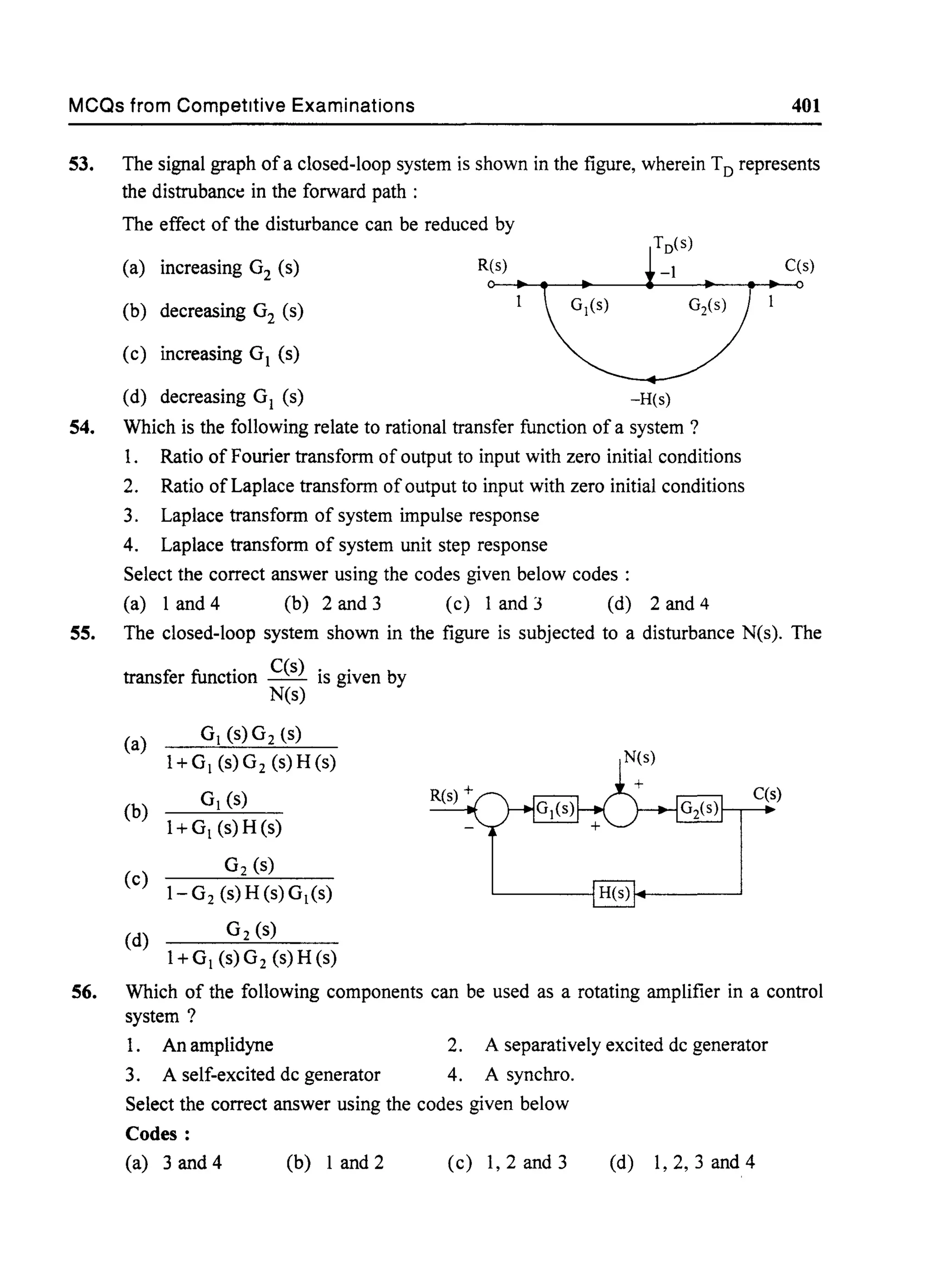
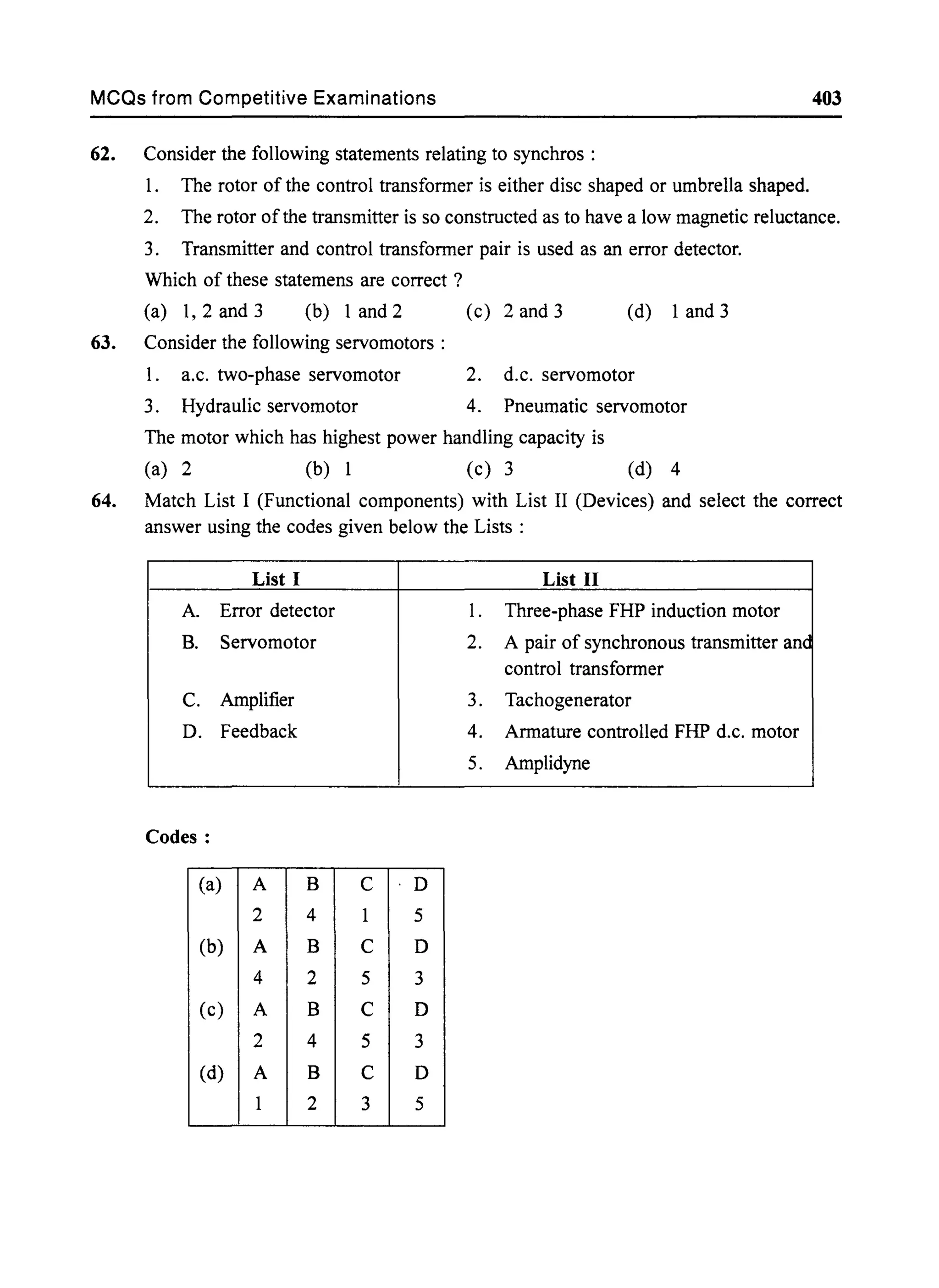
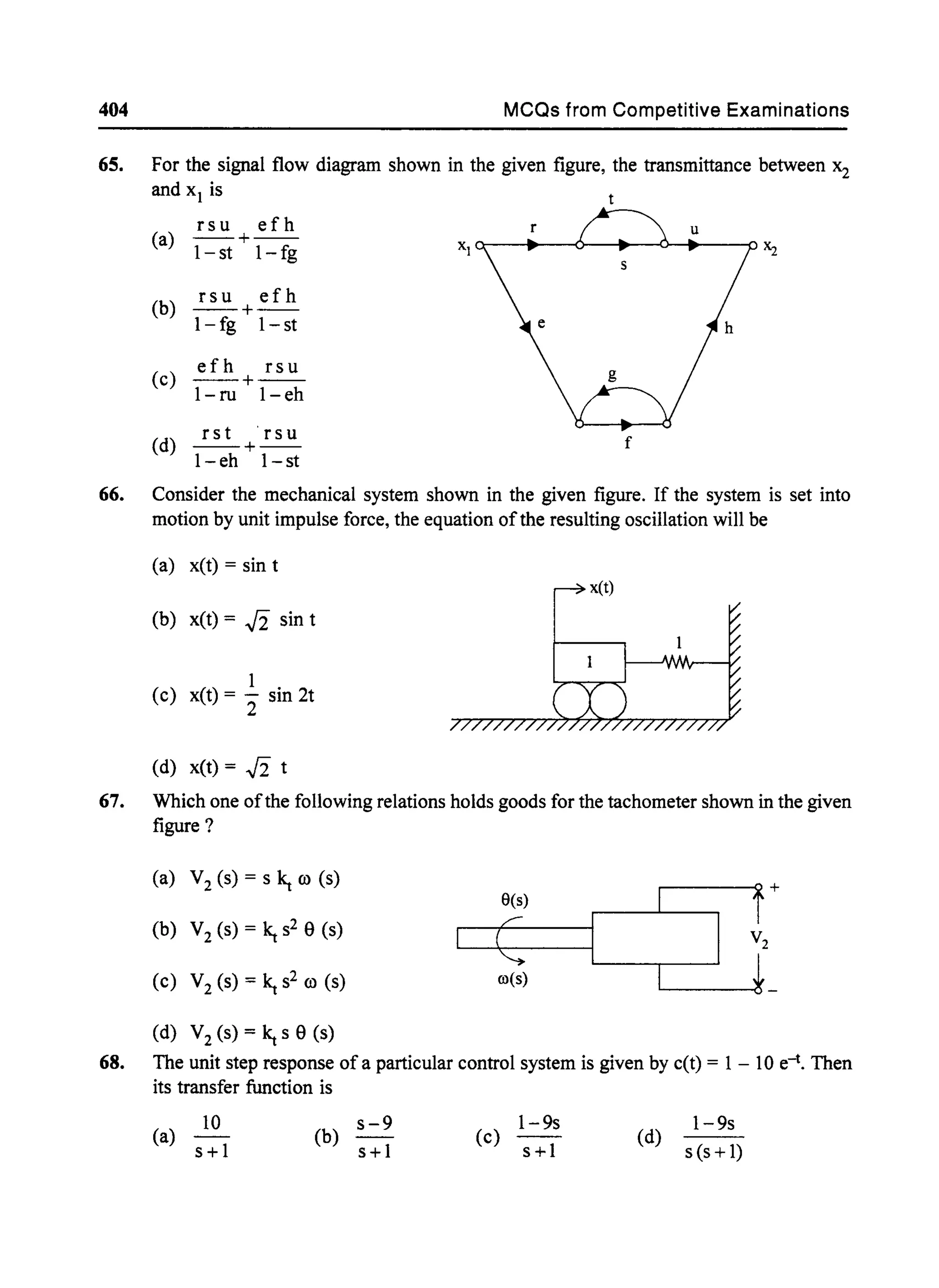
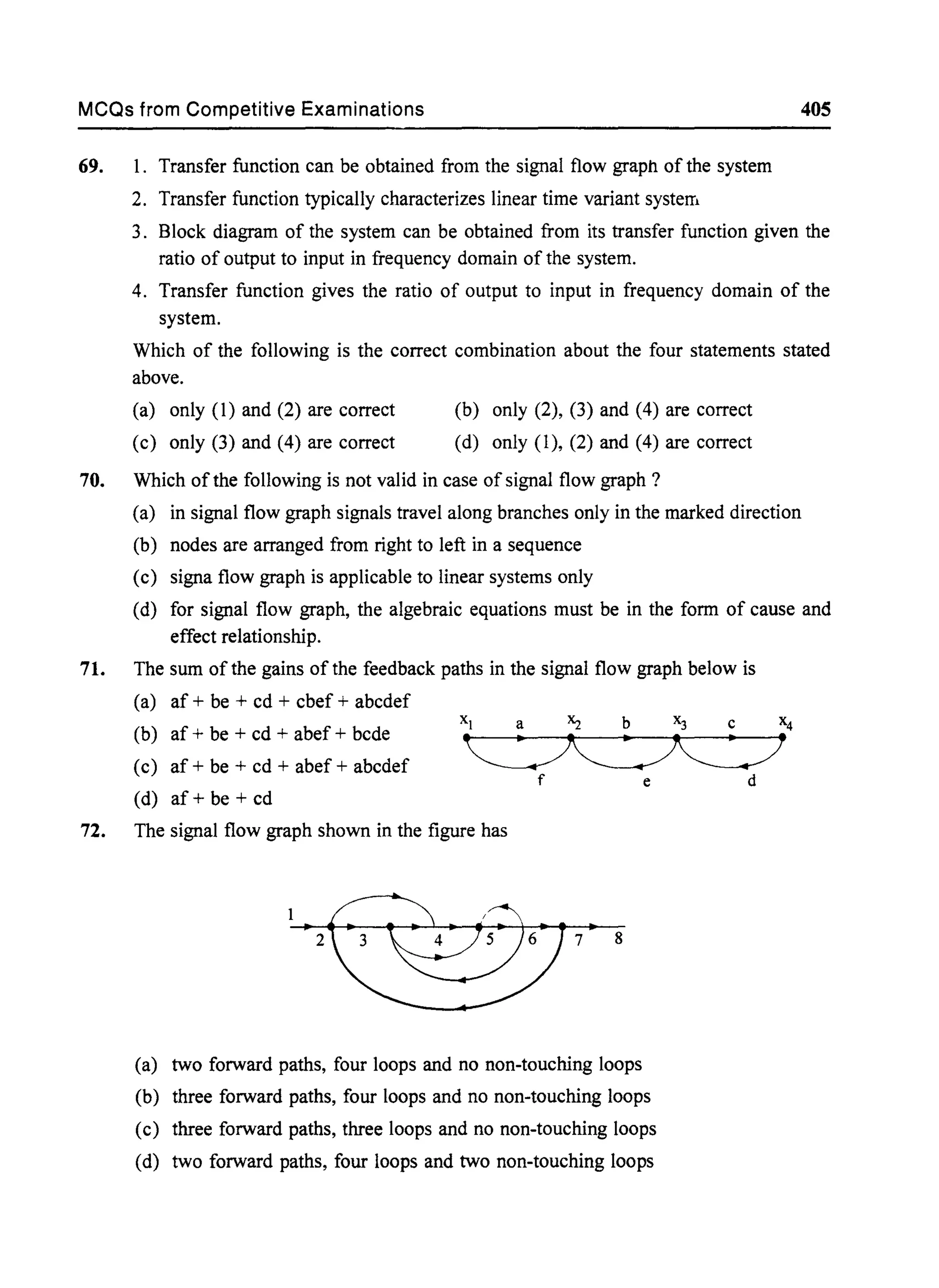
420. MCQs from Competitive Examinations 411
6. For the system shown in figure with a damping ratio ~ of 0.7 and an undamped natural
frequency OJn of 4 rad/sec; the values of K and a are
(a) K = 4, a = 0.35
(b) K = 8, a = 0.455
(c) K = 16, a = 0.225
(d) K =64, a =0.9
C(s)
7. A unity feedback system has open-loop transfer function O(s). The steady-state error
is zero for
(a) step input and type-l O(s)
(c) step input and type-O O(s)
(b) ramp input and type-l O(s)
(d) ramp input and type-O O(s)
8. A linear time-invariant system initially at rest, when subjected to a unit-step input, gives
a response yet) = te-t, t> O. The transfer function of the system is,
1
(a) (s+l)2
1
(b)
s (s + 1)2
s
(c) (s+l)2
1
(d) s(s+l)
9. A unity feedback system has open-loop transfer function O(s) = {25/[s (s+6)]). The
peak overshoot in the step-input response of the system is approximately equal to
(a) 5% (b) 10% (c) 15% (d) 20%
10. Introduction of integral action in the forward path of a unity feedback system results in a
(a) Marginally stable system (b) System with no steadystate error
(c) System with increased stability margin (d) System with better speed ofresponse
11. For a unit step input, a system with forward path transfer function O(s) = 2~ and
s
feedback path transfer function
H(s) = (s + 5), has a steady state output of
(a) 20 (b) 5 (c) 0.2 (d) zero
12. Consider a system shown in the given figure:
U(s) O~----l[±]f-----O C(s)
If the system is disturbed so that c(O) = I, then c(t) for a unit step input will be
(a) 1 + t (b) 1 - t (c) 1 + 2t (d) 1 - 2t

421. 412 MCQs from Competitive Examinations
13. What will be the closed-loop transfer function ofa unity feedback control system whose
14.
step response is given by c(t) = k[1 - 1.66 e-8t sin (6t + 37°)]?
lOOk
(a) S2 + 16s + 100
10
(b) S2 + 16s + 100
k
(c) S2 + 16s + 100
10k
(d) S2 +8s+100
K
The transfer function of a control system is given as T(s) = - - - -
s2+4s+K
where K is the gain of the system in radians/Amp.
For this system to be critically damped, the value ofK should be
(a) 1 (b) 2 (c) 3 (d) 4
15. A linear system, initially at rest, is subject to an input signia r(t) = 1 - e-t
(t ~ 0)
The response of the system for t > 0 is given by c(t) = 1 - e-2t
The transfer function of the system is
(s+ 2)
(a) (s +1)
(b) (s +1)
(s +2)
(c) 2(s +1)
(s +2)
l(s +1)
(d) 2(s +2)
16. If the time response of a system is given by the following equation
y(t) = 5 + 3 sin (rot + (1) + e-3t sin (rot + (2) + e-5t
then the steady-state part of the above response is given by
(a) 5 + 3 sin (rot + (1) (b) 5 + 3 sin (rot + (1) + e-3t sin (rot + (2)
(c) 5 + e-5t (d) 5
17. The impulse response of a system is 5 e-10t• Its step response is equal to
(a) 0.5 e-10t (b) 5(1 - e-10t) (c) 0.5 (l - e-10l) (d) 10(1 - e-1Ot)
18. The transfer function of a system is ~. When operated as a unity feedback system,
l+s
the steady-state error to a unit step input will be
(a) zero
1
(b) 11 (c) 10 (d) infinity

422. MCQs from Competitive Examinations 413
19.
K
A unity feedback second order control system is characterised by G(s) = - - -
s(Js +B)
Where J = moment of inertia, K = system gain, B =viscous damping coefficient. The
transient response specification which is NOT affected by variation of system gain is
the
(a) peak overshoot
(c) settling time
(b) rise time
(d) damped frequency of oscillations
20. In the control system shown in the given figure, the controller which can give zero
steady-state error to a ramp input, with K = 9 is
21.
22.
(a) proportional type +
(b) integral type
(c) derivative type
(d) proportional plus derivative type.
A linear second-order system with the transfer function G (s) = 2 49 is initially
s +16s+49
at rest and is subject to a step input signal. The response of the system will exhibit a
peak overshoot of
(a) 16% (b) 9% (c) 2% (d) zero
100(s + 5)(s + 50)
A system has the following transfer function: G (s) = -s4-:-(-s-+'::"'10-)-(s-=-2':"'-+-3-s-+:""'10-)
The type and order of the systems are respectively
(a) 4and9 (b) 4and7 (c) 5and7 (d) 7and5
23. When the input to a system was withdrawn at t = 0, its output was found to decrease
exponentially from 1000 units to 500 units in 1.386 seconds. The time constant of the
system is
(a) 0.500 (b) 0.693 (c) 1.386 (d) 2.000
24. For the system shown in the given figure, the steady-state value of the output c(t) is
(a) 0
(b)
(c) 00
(d) dependent of the values ofK and K
INPUT
1 + 0.02s
OUTPUT
C(s)

423. 414 MCQs from Competitive Examinations
25. The unit impulse response of a linear time-invariant second-order system is :
get) = 10 e-8t sin 6t (t ~ 0).
26.
27.
The natural frequency and the damping factor of the system are respectively
(a) 10 radls and 0.6 (b) 10 radls and 0.8
(c) 5 rad/s and 0.6 (d) 6 rad/s and 0.8
[- a ±jb] are the complex conjugate roots of the characteristic equation of a second
order system. Its damping coefficient and natural frequency will be respectively
b b
(a) and ~a2 + b2 (b) and a2 + b2
~a2 + b2 ~a2 + b2
a a
(c) and ~a2 + b2 (d) and a2 + b2
~a2 + b2 ~a2 + b2
10(1+4s)
A unity feedback control system has a forward path transfer function G(s) = 2 ( ).
s l+s
t
2
If the system is subjected to an input ret) = 1 + t + 2" (t ~ 0), the steady-state error of
the system will be
(a) zero (b) 0.1 (c) 10 (d) infInity
28. In the system shown in the given fIgure, ret) = I + 2t (t> 0). The steady-state value of
the error e(t) is equal to
(a) zero C(t)
(b) 2/10 ret)
(c) 10/2
(d) infInity
29. The steady state error due to a ramp input for a type two system is equal to
(a) zero (b) infInite
(c) non-zero number (d) constant
30. A second order control system is defIned by the following differential equation:
d2
c(t) d c(t)
4 ~ + 8 dt2 + 16 c(t) = 16 u(t)
The damping ratio and natural frequency for this system are respectively
(a) 0.25 and 2 rad/s (b) 0.50 and 2 rad/s
(c) 0.25 and 4 rad/s (d) 0.50 and 4 rad/s

424. MCQs from Competitive Examinations 415
31. The open loop transfer function of a unity feedback system is given by _K_. If the
s(s +1)
32.
33.
34.
35.
36.
value of gain K is such that the system is critically damped, the closed loop poles ofthe
system will lie at
(a) -0.5 and -0.5 (b) ±jO.5 (c) 0 and-l (d) 0.5 ±jO.5
A linear time invariant system, initially at rest when subjected to a unit step input gave a
response c(t) = te-t (t :::: 0). The transfer function of the syste is
s 1 1 1
(a)
(s + 1)2
(b)
s(s+ 1)2 (c) (s + 1)2 (d) s(s+l)
The steady-state error resulting from input ret) = 2 + 3t + 4t2 for given system is
(a) 2.4
+
(b) 4.0
"')1(c) zero
(d) 3.2
In the derivative error compensation
(a) damping decreases and settling time decreases
(b) damping increases and settling time increases
(c) damping decreases and settling time increases
(d) damping increases and settling time decreases
>
10
52
(4+5)
J
A second order system exhibits 100% overshoot. Its damping coefficient is
(a) equal to 0 (b) equal to 1 (c) less than 1 (d) grater than 1
d2y dy
For a second order system 2 -2 + 4 - + 8y = 8x
dt dt
The damping ratio is
(a) 0.1 (b) 0.25 (c) 0.333 (d) 0.5
37. The feedback control system shown in the given figure represents a
(a) Type 0 system
(b) Type 1 system
(c) Type 2 system
(d) Type 3 system

425. 416 MCQs from Competitive Examinations
38. In the type 1 system, the velocity error is
(a) Inversely proportional to bandwidth
(b) Directly proportional to error constant
(c) Inversely proportional to error constant
(d) Independent of error constant
39. In position control systems, the device used for providing rate-feedback voltage is
called
(a) potentiometer
(c) synchro transformer
(b) synchro transmitter
(d) technogenerator
40. A unity feedback control system has a forward path transfer function equal to 42.25
s(s+6.5)
The unit step response ofthis system starting from rest, will have its maximum value at
a time equal to
(a) 0 sec (b) 0.56 sec (c) 5.6 sec (d) infinity
41. Match the system open-loop transfer functions given in List-I with the steady-state
errors produced for a unit ramp input. Select the correct answer using the code given
below the lists:
List-I List-II
30
A.
S2 +6s+9
l. Zero
B.
30
2. 0.2- -
S2 +6s
c.
30
- - 3. 0.3
S2 +9s
s+l
D. -- 4. Infmity
S2
Codes:
(a) A B C D (b) A B C D
2 3 4 4 3 1 2
(c) A B C D (d) A B C D
3 2 4 4 2 3

426. MCQs from Competitive Examinations 417
42.
43.
A transfer function G(s) has the pole-zero plot as shown in the given figure. Given that
the DC gain is 2, the transfer function G(s) will be given by
(a)
2 (s + 1)
(b)
5(s+l) x - -
S2 + 4s + 5 S2 + 4s + 4
(c)
10(s+l)
(d)
10(s+l) -2 I -1
S2 + 4s + 5 (s + 2)2
I
'" - - ---:i
A plant has the following transfer function G(s) = (S2 + 0.2s + 1)
For a step input it is required that the response settles to within 2% ofits final value. The
plant settling time is
(a) 20 sec (b) 40 sec (c) 35 sec (d) 45 sec
44. Match List-I with List-II and select the correct answer using the codes given below the
lists:
List-I (Transfer function) List-II (Controller)
A.
K S+K2
K3
1. P-controller
B.
KS2 + K2s + K3
2. PI-controller
K4s
C.
Ks+K2
3. PO-controller
K3S
o.
Ks
K2s
4. PID-controller
Codes:
(a) A B C 0 (b) A B C 0
3 4 2 1 4 3 2 1
(c) A B C 0 (d) A B C 0
3 2 4 4 2 3
45. Consider the following expressions which indicate the step or impulse response of an
initially relaxed control system:
1. (5 - 4e-2l) u(t) 2. (e-2t + 5) u (t)
3. 8(t) + 8e-2t u(t) 4. 8(t) + 4e-2t u(t)
Those which correspond to the step and impulse response of the same system include
(a) 1 and 3 (b) 1 and 4 (c) 2 and 4 (d) 2 and 3

427. 418 MCQs from Competitive Examinations
46. Assuming the transient response of a second-order system to be given by
-41
c(t) = 1 - b sin (ron ~ + 8) the settling time for the 5% criterion will be
1-82
1
(a) - sec
4
3
(b) - sec
4
5
(c) - sec
4
(d) 4 sec
47. Consider the systems with the following open-loop transfer functions:
1.
36
2.
s(s +3.6)
100
s(s + 5)
3.
6.25
s(s + 4)
The correct sequence of these systems in increasing order of the time taken for the
unit-step response to settle is
(a) 1, 2, 3 (b) 3, 1,2 (c) 2, 3, 1 (d) 3,2, 1
48. Match List I with List II and select the correct answer using the codes given below the
lists:
List I (Characteristic equations) List II (Nature of damping)
A. s2 + ISs + 56.25 1. Undamped
B. s2 + 5s + 6 2. Underdathped
C. s2 + 20.25 3. Critically damped
D. s2 + 4.5s + 42.25 4. Overdamped
Codes:
(a) A B C 0 (b) A B C 0
3 4 2 2 3 4
(c) A B C 0 (d) A B C 0
4 3 2 3 4 2
49. For the control system in the given figure to be critically damped the value of the gain
'K' required is :
r'l C(s)
(a) (b) 5.125
r(c) 6.831 (d) 10
+____K__. S2 +7s + 2 :

428. MCQs from Competitive Examinations 419
50. Match List I with List II and select the correct answer using the codes given below the
lists:
List I List II
A. Derivative control 1. Improved overshoot response
I
B. Integral control 2. Less steady-state errors
C. Rate feedback control 3. Less stable
D. Proportional control 4. More damping
Codes:
(a) A B C D (b) A B C D
2 3 4 2 3 4
(c) A B C D (d) A B C D
4 3 2 2 4 3
51. A typical control system is shown in, the given figure.
1
52.
Assuming R(s) = -, the steady-state error is given by
s
(a) 1+ K (b) K
(c) zero (d) 1
10
A system has open-loop transfer function G(s) = - - - - -
s (s +l)(s + 2)
C(s)
3
What is the steady state error when it is subjected to the input r (t) = 1 + 2t + 2" t2 ?
(a) zero (b) 0.4 (c) 4 (d) infinity
53. Consider a unit feedback control system shown in the given figure. The ratio of time
constants of open-loop response to closed loop response will be
(a) 1: 1
(b) 2: 1
(c) 3: 2
(d) 2: 3
C(s)

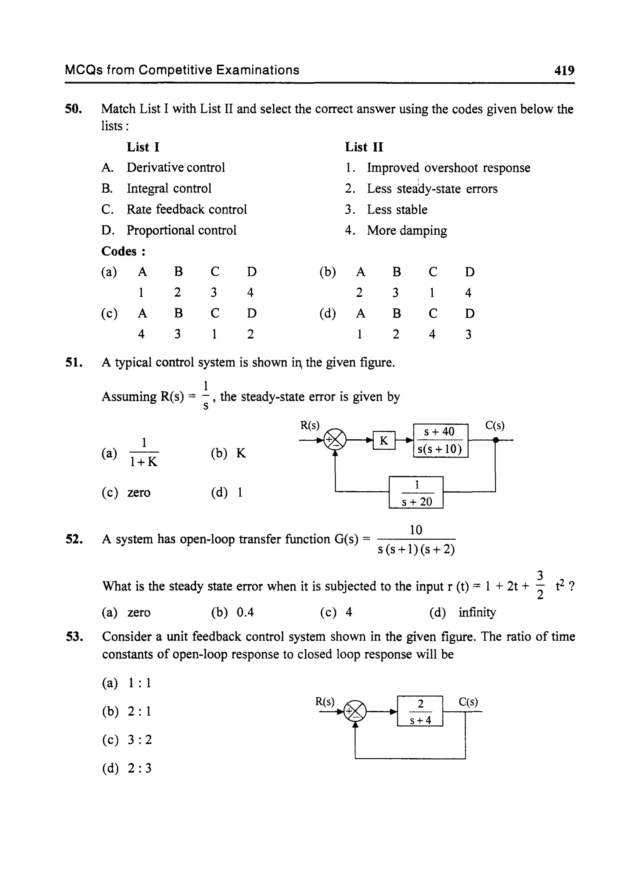
429. 420 MCQs from Competitive Examinations
54. Consider the following overall transfer function for a unity feedback system :
55.
56.
57.
4
S2 + 4s + 4
Which of the following statements regardmg this system are correct ?
1. Position error constant ~ for the system is 4.
2. The system type one.
3. The velocity error constant ~ for the system is finite.
Select the correct answer using the codes given below :
Codes:
(a) 1, 2 and 3 (b) 1 and 2 (c) 2 and 3 (d) 1 and 3
A first order system is shown in the given figure. Its time response to a unit step input
is given by
(a) c(t) = [liT] [e-tlT]
(b) c(t) = T (l - e-tlT) R(s)
·11+lST 1
C(s)
•(c) c(t) = (1 - e-tlT)
(d) c(t) = Te-tiT
16(s + 2)
For a unity feedback system, the open-loop transfer function is G(s) = 2 ) ( )
s (s +1 s + 4
What is the steady-state error if the input is, r (t) = (2 + 3t + 4t2) u(t) ?
(a) 0 (b) 1 (c) 2 (d) 3
. C(s) 4
A system has a transfer functIOn -- = -2----
R(s) s +1.6s+4
For the unit step response, the setling time (in seconds) for 2% tolerance band is
(a) 1.6 (b) 2.5 (c) 4 (d) 5
58. Consider the following statements :
1. The derivative control improves the overshoot of a given system.
2. The derivative control reduces steady-state error.
3. Integral control reduces steady-state error.
4. Integral control does not affect stability of the system.
5. Integral control improves the overshoot of the system.
Of these statements
(a) 1 and 3 are correct
(c) 2, 4 and 5 are correct
(b) 1, 2 and 5 are correct
(d) I, 3 and 5 are correct

430. MCQs from Competitive Examinations 421
59. In the case of a second order system described by the differential equation,
(where 9i and 90
are the input and output shaft angles), the natural frequency is given by
(a) ~ (b) If (c) JKi (d) ~K-J
60. A transducer has two poles as shown in the figure. The zeros are at infinity and the DC
gain is 1. The steady-state output of the transducer for a unit step input will be
1m
(a)
4
x:- t,
,
(b) ,
2
I
ReI
45°
/
1
/
(c)
,
Ii
x,
(d)
61. The velocity error constant ~ of a feedback system with closed-loop transfer function
C(s) = __G....:...(s..:...)_ is
R(s) 1+G(s) H(s)
(a) ~ = ~l11J s G(s) H(s)
(c) ~ = ~l11J s G(s)
L· G(s)
(b) ~ = s':'11J s --"'--'--
1+ G(s) H(s)
(d) ~ = ~l~ s [1 + G(s) H(s)]
62. The settling time of a feedback system with the closed-loop transfer function
(a) ts = 2/(~ O)n)
(c) ts = 4/(~ O)n)

431. 422 MCQs from Competitive Examinations
63. A second order under-damped system exhibited a 15% maximum overshoot on being
excited by a step input r (t) = 2u(t), and then attained a steady-state value of 2
(see figures given). If, at t = to' the input were changed to a unit step r (t) = u (t), then
its time response C (t) would be similar to
(a) 3 - - - - - - - - - - - ~) 3 ----------- ----
i 2 - i 2 -
C(t) C(t)
o to t~ to t---+
(c) 3 (d) 3 - - - - - - - - - - - - - - -
i 2 - i 2
C(t) C(t)
o to t~
64. The response c(t) of a system is described by the differential equation
d2
c(t) dc(t)
- - + 4 - - + 5c(t) = 0
dt2
dt
The system response is
(a) undamped
(c) critically damped
(b) underdamped
(d) oscillatory
65. The system with the open-loop transfer function G(s) H(s) = _1_ is
s(1 +s)
(a) type 2 and order 1
(c) type 0 and order 0
(b) type 1 and order 1
(d) type 1 and order 2
to t---+

432. MCQs from Competitive Examinations 423
66. The transfer function G (s) of a PID controller is
67.
68.
69.
(a) K (1 +_1_+ TdS)
TIs
The industrial controller having the best steady-state accuracy is
(a) a derivative controller (b) an integral controller
(c) a rate feedback controller (d) a proportional controller
e-S
A step input is applied to a system with the transfer function G (s) = . The
1+0.5s
output response will be
(a) (b)
1
----------g/- ~
(c) (d)
The open-loop transfer function G(s) of a unity feedback control system is _1_
s(s +1)
The system is subjected to an input r(t) = sin t. The steady-state error will be
(a) zero (b) 1
(d) J2 sin (t +~)
70. A second order, system has the damping ratio; and undamped natural frequency of
oscillation ron' The settling time at 2% tolerance band of the system is

433. 424 MCQs from Competitive Examinations
71. Consider the following statements:
A proportional plus derivative controller
1. has high sensitivity
2. increases the stability of the system
3. improves the steady-state accuracy
Which of these statements are correct ?
(a) 1, 2 and 3 (b) 1 and 2 (c) 2 and 3 (d) 1 and 3
72. Which one of the following is the steady-state error for a step input applied to a unity
. . 10
feedback system with the open loop transfer functlOn O(s) = 2 ?
s +14s+50
(a) ess = 0 (c) ess = 0.2
73. With derivative output compensation, for a specified velocity error constant,
(a) Overshoot for a step input increases
(b) The settling time is decreased
(c) The natural frequency decreases
(d) Peak time increases
74. Which of the following is not a desirable feature ofa modem control system
(a) Quick response (b) accuracy
(c) correct power level (d) no oscillation
75. Damping factor and undamped natural frequency for the position control system is
given by
(a) 2.JKj, .JKj respectively.
f
(c) 2.JKj,,JK / J respectively.
Where, K = torsional stiffness
J = Moment of Inertia
K
(b) 2fJ' ~K/J respectively
J
(d) 2..JKi'.JKj respectively.
and f = Coefficient viscous friction
76. In the derivative error compensation
(a) damping decreases and settling time decreases
(b) damping increases and settling time increases
(c) damping decreases and settling time increases
(d) damping increases and settling time decreases.

434. MCQs from Competitive Examinations 425
77. A control system having unit damping factor will give
(a) critically damped response (b) oscillatory response
(c) undamped response (d) no response.
78'. Which ofthe following will not decrease as a result ofintroduction ofnegative feedback?
(a) Instability (b) Band width
(c) Overall gain (d) Distortion
79. Consider the following statements regarding time domain analysis of control systems:
1. Derivative control improves systems transient performance.
2. integral control does not improve system steady state performance
3. integral control can convert a second order system into a third order system
Of these statements
(a) 1 and 2 are correct
(c) 2 and 3 are correct
(b) 1 and 3 are correct
(d) I, 2 and 3 are correct
80. The open-loop transfer transfer function of a unity feedback control system is given by
K
G(s) = s(s +1)
Ifthe gain K is increased to infinity, then the damping ratio will tend to become
1
(a) .fi (b) 1 (c) 0 (d) ex)
81. The system shown in the given figure has a unit step input. In order that the steady-state
error is 0.1, the value of K required is
c
(a) 0.1 (b) 0.9
(c) 1.0 (d) 9.0
82. The system shown in the given figure has second order response with a damping ratio
of 0.6 and a frequency of damped oscillations of 10 rad/sec. The values of Kl and K2
are respectively
(a) 12.5 and 15
R~S(S+1;+K2sTC(b) 156.25 and 15
(c) 156.25 and 14
(d) 12.5 and 14

435. 426 MCQs from Competitive Examinations
Chapter 4
1. None of the poles of a linear control system lies in the right half of s plane. For a
bounded input the output of this system
(a) is always bounded (b) could be unbounded
(c) always tends to zero (d) none of the above
2. The number of roots of the equation 2s4 + s3 + 3s2+ 5s + 7 = 0 that lie in the right half
of s plane is
(a) zero (b) one (c) two (d) three
3. The characteristic equation of a feedback control system is 2s4 + s3 + 3s2 + 5s + 10 = O.
The number of roots in the right halfofs-plane are
(a) zero (b) 1 (c) 2 (d) 3
4. Consider a system shown in the given figure with
5.
~t~_-_-_-_"@_G(_S):_-_-_-~~.
What values of 'K' and 'a' should be chosen so that the system oscillates ?
(a) K=2,a=1 (b) K=2, a=0.75 (c) K=4,a=1 (d) K=4,a=0.75
k
The open loop transfer function of a system is given by G(s) = s(s + 2)(s + 4) . The
maximum value of k for which the unity feedback system will be stable, is
(a) 16 (b) 32 (c) 48 (d) 64
6. The characteristic equation 1 + G(s) R(s) = 0 of a system is given by
s4 + 6s3 + 11s2 + 6s + K = 0
For the system to remain stable, the value ofgain K should be
(a) zero (b) greater than zero but less than 10
(c) greater than 10 but less than 20 (d) greater than 20 but less than 30
7. The open-loop transfer function of a unity feedback control system is
30
G(s) R(s) = s(s + l)(s + T) where T is a variable parameter. The closed loop system will
be stable for all values of
(a) T> 0 (b) 0 < T < 3 (c) T> 5 (d) 3<T<5

436. MCQs from Competitive Examinations 427
8. The open-loop transfer function of a unity-feedback control system is :
K(s + 10)(s + 20)
G (s) == s2(s+2)
The closed-loop system will be stable if the value of K is
(a) 2 (b) 3 (c) 4 (d) 5
9. The characteristic equation of a feedback control system is s3 + Ks2 + 5s + 10 == O.
For the system to be critically stable, the value ofK should be
(a) 1 (b) 2 (c) 3 (d) 4
10. The control system shown in the given figure has an internal rate feedback loop. The
closed-loop system for open and close conditions of switch will be respectively
(a) unstable and stable
R(s) C(s)
(b) unstable and unstable
(c) stable and unstable
(d) stable and stable
11. For the block diagram shown in the given figure, the limiting values ofK for stability of
inner loop is found to be X < K < Y. The overall system will be stable if and only if
12.
(a) 4X < K < 4Y R(s) + K C(s)
(b) 2X < K < 2Y (s-a)(s+2a)(s+3a)
(c) X<K<Y
X Y
(d)-<K<-
2 2
A feedback control system is shown in the given figure. The system is stable for all
positive values of K, if
(a) T == 0
(b) T < 0
(c) T> 1
(d) O<T<1
C(s)
R(s)
13. The characteristic equation of a system is given by 3s4 + 10s3 + 5s2 + 2 == O. This
system is
(a) stable (b) marginaly stable (c) unstable (d) neither (a), (b) nor (c)
14. The characteristic equation s3 + 3s2 + 3s + k == 0 is stable for which value of k ?
(a) - 6 (b) 15 (c) 5 (d) 12

437. 428 MCQs from Competitive Examinations
15. Which ofthe following statement about the equation below, for Routh Hurwitz criterion
is true?
2S4 + s3 + 3s2 + 5s + 10 = 0
(a) It has only one root on the imaginary axis
(b) It has one root in the right half of the s-plane
(c) The system is unstable
(d) The system is stable.
16. When all the roots ofthe characteristic equation are found in the left halfofs-plane, the
system response due to initial condition will
(a) increase to infinity as time approaches infinity
(b) decreases to zero as time approaches infinity
(c) remain constant for all time
(d) be oscillating
17. Match List-I with List-II and select the correct answer by using the codes given below
the lists:
List-I (Characteristic Root Location) List-II (System characteristic)
A. (-1 + j), (-1 -j) 1. Marginally stable
B. (-2 + j), (-2 -j), (2j), (-2j) 2. Unstable
C. -j, j, -1, 1 3. Stable
Codes:
(a) A B C (b) A B C
1 2 3 2 3 1
(c) A B C (d) A B C
3 2 1 3 2
18. A control system is as shown in the given figure. The maximum value of gain K for
which the system is stable is
(a) J3
(b) 3
(c) 4
(d) 5

438. MCQs from Competitive Examinations 429
19. If the open-loop transfer function of the system is G(s) H(s) = K(s +10) ,
s (s +8)(s +16) (s + 72)
then a closed loop pole will be located at s = - 12 when the value of K is
(a) 4355 (b) 5760 (c) 9600 (d) 9862
20. Consider the following statements regarding the number of sign change in the first
column of Routh array in respect of the characteristic equation s2 + 2as + 4 :
1. If a = + 1;, where I; = near zero, number of sign changes will be equal to zero.
2. If a = 0, the number of sign change will be equal to one.
3. If a = -I;, where I; = near zero, the number of sign changes will be equal to two
Of these statements
(a) 1, 2 and 3 are correct
(c) 2 and 3 are correct
(b) 1 and 2 are correct
(d) 1 and 3 are correct
21. How many roots of the characteristic equation s5 + s4 + 2s3 + 2s2 + 3s + 15 = 0 line in
the left half of the s-plane ?
22.
23.
(a) 1 (b) 2 (c) 3 (d) 5
The first column of a Routh array is
s5 1
S4 2
s3
3
2
s2 1
- -
3
sl 10
sO 2
How many roots of the corresponding characteristic equation are there in the left-half
of the s-plane ?
(a) 2 (b) 3 (c) 4 (d) 5
1 K
Consider a negative feedback system where, G(s) = (s + 1) , H(s) =
The closed-loop system is stable for
(a) K> 20
(c) 8:sK:S14
(b) 15 < K < 10
(d) K < 6
s(s + 2)
24. The value ofK for which the unity feedback system G(s) = K crosses the
s (s + 2) (s + 4)
imaginary axis is
(a) 2 (b) 4 (c) 6 (d) 48

439. 430 MCQs from Competitive Examinations
25. While forming Routh's array, the situation of a row of zeros indicates that the
system
(a) has symmetrically located roots (b) is not sensitive to variations in gain
(c) is stable (d) unstable
26. The closed loop system shown above becomes marginally stable if the constant K is
chosen to be
(a) 10
(b) 20
(c) 30
(d) 40
27. A closed-loop system is shown in the following figure:
The largest possible value of Pfor which this system would be stable is :
(a)
10
(b) 1.1 S3 +4S2 +3s+1
(c) 1.2
P
(d) 2.3
Output
28. First column elements of the Routh's tabulation are 3,5 ~, ~, 2. It means that there
(a) is one root in the left half of s-plane
(b) are two roots in the left half of s-plane
(c) are two roots in the right half of s-plane
(d) is one root in the right half of s-plane
29. The open-loop transfer fucntion of unity feedback control system is
K
G(s) = , 0 < a < b
s(s+ a)(s + b) -
The system is stable if
(a+ b)
(a) 0 <K<--
ab
(c) O<K<ab(a+b)
ab
(b) O<K<--
(a + b)
a
(d) 0 < K < b (a + b)
•

440. MCQs from Competitive Examinations 431
30. Which one ofthe following characteristic equations can result in the stable operation of
the feedback system ?
(a) s3 + 4s2 + S - 6 = 0 (b) s3 - s2 + 5s + 6 = 0
(c) s3 + 4s2 + lOs + 11 = 0 (b) s4 + s3 + 2s2 + 4s + 6 = 0
31. Consider the following statements :
Routh-Hurwitz criterion gives
1. absolute stability
2. the number of roots lying on the right half of the s-plane
3. the gain margin and phase margin
Which of these statements are correct ?
(a) 1, 2 and 3 (b) 1 and 2 (c) 2 and 3 (d) I and 3
32. The given characteristic polynomial s4 + s3+ 2s2 + 2s + 3 = 0 has
(a) zero roots in RHS of s-plane
(c) two roots in RHS of s-plane
(b) one root in RHS of s-plane
(d) three roots in RHS of s-plane
33. For making an unstable system stable
(a) gain of the system should be increased
(b) gain of the system should be decreased
(c) the number of zeros in the loop transfer function should be increased
(d) the number of poles in the loop transfer function should be increased.
34. Which of the following system is unstable?
(b) G(s) H(s) = K(s + 1)
S2(S + 4)(s + 5)
K(s + 2)
(c) G(s) H(s) = (s+I)(s-3)
K
(d) G(s) H(s) = 3
(Ts +1)
K>99
K>2
-1 < K < 8 T>O

441. 432 MCQs from Competitive Examinations
35. The characteristic equation of a closed-loop system is given by :
s4 + 6s3 + 11s2 + 6s + K = O.
Stable closed-loop behaviour can be ensured when gain K is such that
(a) 0<K<10 (b) K> 10 (c) -oo:sK<oo (d) 0<K:s20
36. By a suitable choice of the scalar paramter K, the system shown in the given figure can
be made to oscillate continuously at a frequency of
(a) 1 rad/s
(b) 2 rad/s
(c) 4 rad/s
(d) 8 rad/s
c(t)
37. The open-loop transfer functions with unity feedback are given below for different
38.
systems:
2
G(s) =
2
1. G(s) = - 2.
s+2 s(s + 2)
2 2(s + 1)
3. G(s) =
ss +2)
4. G(s) -
s(s + 2)
Among these systems the unstable system is
(a) 1 (b) 2 (c) 3 (d) 4
. . K(s+10)
The open-loop transfer function of a control system IS given by ---'----
s(s + 2)(s + a)
The smallest possible value of 'a' for which this system is stable under unity feedback
closed-loop condition for all positive values ofK is
(a) 0 (b) 8 (c) 10 (d) 12
39. The open-loop transfer function ofa unity negative feedback control system is given by
G(s) = K(s + 2)
(s + l)(s -7)
For K > 6, the stability characteristic ofthe open-loop and closed-loop configurations of
the system are respectively
(a) stable and stable (b) unstable and stable
(c) stable and unstable (d) unstable and unstable

442. MCQs from Competitive Examinations 433
Chapter 5
1.
2.
K
jroV Jro
A un~ty fe
J
:j8Ck ~ on open loopfSfer function, G(s) = s' . The root I)iSplot is:
(a) (J (b) (J (c) ~ (d) (J
K(s + 2)
Given a unity feedback system with open-loop transfer function G(s) = (s + )2
The correct root-locus plot of the system is
r~
(b)~_1
r!(a) --O~...~~~--+-~
-2 -I
(c) • e)-~--I--+--..
r
jro
-2
~ (d)
3. The closed-loop transfer function of a feedback control system is given by
C(s) K
=----::------
R(s) S2 +(3+K)s+2
Which one of the following diagrams represents the root-locus diagram of the system
for K > O?
8
i
::.G
(a)
K=Q K=Q
;...;
,(,
8
jro
(c)
K=Q
jro
(b)
(J
K-+oo
(J
(d)
oo+-K
K=Q K=Q
00 +- K K=Q K=Q
jro
jro
(J
K-+oo

443. 434 MCQs from Competitive Examinations
4. The open-loop transfer function of a feedback control system is given by
5.
6.
7.
K(s+ 2)
G(s) H(s) = s(s + 4)(S2 + 4s + 8)
In the root-locus diagram ofthe system, the asymptotes ofthe root loci for large values
ofK meet a point in the s-plane. Which one ofthe following is the set ofco-ordinates of
that point?
(a) (-1.0) (b) (-2.0) (d) (2, 0)
K
If the characteristic equation of a closed-loop system is 1 + S(s + l)(s + 2) = 0 the
centroid of the asymptotes in root-locus will be
(a) zero (b) 2 (c) - 1 (d) - 2
The root-locus of a unity feedback system is shown in the given figure. The open-loop
transfer function of the system is
(a)
K
s (s + l)(s + 3)
~
(b)
K (s + 1)
s (s + 3) s-plane
K (s+3)
(c) Re
s (s + 1)
(d) Ks
(s+1)(s+3)
The open-loop transfer function of a feedback control system is
S(S2 +3s+6) .
K
The break-away point(s) of its root-locus plot
(a) exist at (-1 ±j 1) (b) exist at H± MJ
(c) exists at origin (d) do not exist

444. MCQs from Competitive Examinations 435
8. Match List-I with List-II in respect of the open-loop transfer function
K(s + 10)(s2 + 20s + 500)
G(s) H(s) '= (20)( 2 and select the correct answer using the codes
s s+ s+50)(s +4s+5)
given below the lists:
List-I (Types of loci) List-II (Numbers)
(A) Separate loci 1. One
(B) Loci on the real axis 2. Two
(C) Asymptotes 3. Three
(D) Breakaway points 4. Five
Codes:
A B C D A B C D
(a) 3 4 2 (b) 3 4 1 2
A B C D A B C D
(c) 4 3 2 (d) 4 3 2
9. The characteristic equation of a linear control system is s2 + 5Ks + 10 '= 0
The root-loci of the system for 0 < K < 00 is
(a) jw (b) jw
K=O K=oo
oo~K K=oo (J K=O
K=O K=oo
(c) jw (d) jw
K=O K=oo
K=oo
(J
K~oo
K=O
K=O K=oo
K=O
(J
(J
K~O
10. The characteristic equation ofa feedback control system is given by s3 + 5s2 + (K + 6)s
+ K '= O. In the root loci diagram, the asymptotes ofthe root loci for large 'K' meet at a
point in the s-plane whose coordinates are
(a) (2, 0) (b) (-1,0) (c) (-2,0) (d) (-3,0)

445. 436 MCQs from Competitive Examinations
11. Which of the following are the characteristics ofthe root locus of
K(s +5)
G(s) H(s) = (s + l)(s +3)
1. It has one asymptote 2. It has intersection with jro-axis
3. It has two real axis intersections 4. It h,as two zeros at infinity
Select the correct answer using the codes given below :
Codes:
(a) 1and2 (b) 2and3 (c) 3 and 4 (d) 1 and 3
12. Identify the correct root locus from the figures given below referring to poles and zeros
at ±j 8 and ±j 10 respectively ofG(s) H(s) ofa single-loop control system.
jw jw
(a) (b)
--t-~C1
(c) jw (d)
13. Consider the Root Locus Diagram of a system and the following statements:
1. The open loop system is a second order system
2. The system is overdamped for K > 1
3. The system is absolutely stable for all values of K
Which of these statements are correct ?
(a) 1, 2, and 3 (b) 1 and 3 (c) 2 and 3 (d) 1 and 2
K=}
jw
14. In the root-locus for open-loop transfer function G(s) H(s) = K(s +6) , the break
(s + 3)(s + 5)
away and break in points are located respectively at
(a) - 2 and - 1 (b) - 2.47 and - 3.77
(c) - 4.27 and - 7.73 (d) - 3 and - 4

446. MCQs from Competitive Examinations
K
15. A unity feedback system has G(s) = s (s +1) (s + 2)
In the root-locus, the break-away point occurs between
(a) s = 0 and -1 (b) s =- 1 and - <:Xl
(c) s = - 1 and - 2 (d) s =- 2 and - <:Xl
16. The loop transfer function of a feedback control systme is given by
k
G(s) H(s) = s (s +2) (S2 + 2s + 2)
Number of asymptotes of its root loci is
(a) 1 (b) 2 .(c) 3 (d) 4
437
17. Which of the following are the features of the break away point in the root-locus of a
closed-loop control system with the characteristic equation I + KGI (s) HI (s) = 0 ?
1. It need not always occur only on the real axis.
2. At this point GI (s) HI (s) = O.
dK
3. At this point d; = 0
Select the correct answer using the codes given below:
(a) 1,2 and 3 (b) 1 and 2
(c) 2 and 3 (d) 1 and 3
18. An open-loop transfer function is given by K (s + 3)
s (s +5)
Its root-loci will be as in
(a) (b)
K=ao K=Q K=ao K=Q
-5 -3 Q
(c) (d)
K=Q
-5 K=Q K=Q K=ao
Q

447. 438 MCQs from Competitive Examinations
19. The loop transfer function of a closed-loop system is given by
K
G(s) H(s) = S2 (S2 + 2s + 2)
The angle of departure of the root locus at s = - 1 + j is
(a) zero (b) 900
(c) - 900
(d) - 1800
20. Consider the loop transfer function G(s) H(s) = K(s + 6)
(s+3)(s+5)
In the root-locus diagram, the centroid will be located at
(a) - 4 (b) - 1 (c) - 2 (d) - 3
21. For a unity negative feedback control system, the open-loop transfer function is
K
G(s)= - - - -
s(s + 1) (s + 2)
The root-locus plot of the system is
(a)
jro
s-plane
-2 -1
(c) jro
s-plane
-2 -1
(b)
jro
s-plane
-2 -1
(d) jro
s-plane
22. The intersection ofasymptotes ofroot-loci ofa system with open-loop transfer function
K
G(s) H(s) = i s
~ s(s+l)(s+3)
(a) l.44 (b) l.33 (c) - l.44 (d) - l.33

448. MCQs from Competitive Examinations 439
23. The root locus plot of the system having the loop transfer function
24.
K
O(s) H(s) = has
s(s+4)(s2 +4s+5)
(a) no breakaway point (b) three real breakaway points
(c) only one breakaway point (d) one real and two complex breakaway points
k(s +1)
An open loop transfer function is given by O(s) H(s) = 2 • It has
s(s +2)(s + 2s + 2)
(a) one zero at infinity
(c) three zeros at infinity
(b) two zeros at infinity
(d) four zeros at infinity
25. The intersection of root locus branches with the imaginary axis can be detennined by
the use of
(a) Nyquist criterion
(c) Polar plot
(b) Routh's criterion
(d) None of the above.
26. The root-locus ofa unity feedback system is shown in the figure. The open loop transfer
function is given by
(a)
s(s + 1)(s + 2)
K
(c) K(s+2)
s(s +1)
(b)
(d)
K(s+ 1)
s(s +2)
Ks
(s + l)(s + 2)
27. The characteristic equation of a unity feedback control system is given by
s3 + K1
s2 + S + K2 = 0
Consider the following statements in this regard :
1. For a given value of K1, all the root-locus branches will tenninate at infinity for
variable K2 in the positive direction.
2. For a given value of K2, all the root-locus branches will tenninate at infinity for
variable Kl in the positive direction.
3. For a given value of~, only one root-locus branch will tenninate at infinity for
variable Kl in the positive direction.
Of these statments :
(a) I and 2 are correct
(c) 2 alone is correct
(b) 3 alone is correct
(d) 1 and 3 are correct

449. 440
28.
29.
MCQs from Competitive Examinations
k
The breakaway point of the root locus for the system G(s) H(s) = is
s(s +1)(s +4)
(a) -0.465 (b) -2.87 (c) -1.0 (d) -2.0
The given figure shows the root-locus ofopen-loop transfer function ofa control system.
Index:
o a
30. The loop transfer function GH of a control system is given by
K
GH=-------
s(s +1)(s +2)(s +3)
Which of the following statements regarding the conditions of the system root loci
diagram is/are correct?
1. There will be four asymptotes,
2. There will be three separate root loci.
3. Asymptotes will intersect at real axis at crA = -2/3
Select the correct answer using the codes given below:
Codes:
(a) 1alone (b) 2 alone (c) 3 alone (d) 1,2 and 3
Chapter 6
1. The magnitude plot for a transfer function is shown in figure.
What is the steady-state error corresponding to a unit step input?
(a) 101
1
(c) 41
(b) 100
(d)
40
G, dB
-20 dB dec
401---......
-+----~- logro

450. MCQs from Competitive Examinations
2. The function corresponding to the Bode plot of figure is
if/(d) A= 1 + J/f1
441
3. The asymptotic approximation ofthe log-magnitude versus frequency plot ofminimum
phase system with real poles and one zero is shown in Fig. Its transfer function is
(a)
20(s + 5)
s(s + 2Xs + 25)
dB
10(s+5)
(b)
(S+2)2(S+25) 54
-40dB/dec
--60dB/dec
(c)
20(s + 5)
S2(S + 2Xs + 25)
-40dB/dec
(d)
50(s +5)
s2(s+2Xs+25)
--~~--~2~~5--~~----.m&s
0.1
4. A differentiator has a transfer function whose
(a) phase increases with frequency (b) Amptitude remains constant
(c) Amptitude increases linearly (d) Amptitude decreases linearly with 'f
5. The magnitude-frequency response of a control system is shown in the figure. The
value of Cl) 1 and Cl)2 are respectively
(a) 10 and 200
(b) 20 and 200
(c) 20 and 400
(d) 100 and 400
db
gain +20db/decade
26dB - - -
20dB
-20db/decade

451. 442
6.
MCQs from Competitive Examinations
K 1
The transfer function of a system is given by G Gro) = K < -
(jro)(jroT + 1) , T
Which one of the following is the Bode plot of this function?
(b)
db
-20 db/decade
t
-20 db/decade
,/
t I
20 LogK I
7. The Bode plot shown in the given figure has GGro) as
100
(a) jro(l+ jO.5 roXl + jO.1ro)
Gain db
100
(b) jro(2+ jroX10+ jro)
20 LoglO IG (jro)1 t -20 db decade
20db
2 I 10 100
- - - - - - - - - ro (log scale)
10
(c) jro(1+2jroXl+1Ojro)
10
(d) jro(1+0.5jroXl+O.ljro)
~Odbdecade

452. MCQs from Competitive Examinations 443
8.
9.
10.
11.
1+ s . .
The polar plot of G(s) = 1+ 4s for 0 ~ ro ::: x In G-plane IS
(a) (b) G plane
-I -D.25
0)=00
(c)
G plane
(d)
G plane
0)=00
O)=oc 0)=0
-1 -D.25
A system with transfer function G(s) = _s_ is subjected to a sinusoidal input
(l + s)
r (t) = sin rot. In steady-state, the phase angle of the output relative to the input at ro = 0
and ro = 00 will be respectively ,
(a) 0° and -90° (b) 0° and 0° (c) 90° and 0° (d) 90° and -90°
A system has fourteen poles and two zeros. The slope of its highest frequency asymptote
in its magnitude plot is
(a) - 40 dB/decade (b) - 240 dB/decade
(c) - 280 dB/decade (d) - 320 dB/decade
s+5
The phase angle of the system G(s) = 2 varies between
s + 4s +9
(a) 0° and 90° (b) 0° and -90° (c) 0° and -180° (d) -90° and -180°
12. The following Bode plot represents:
100s2
(a)
(.1+0.ls)3
(b)
1000 S2
(1 + 0.ls)3
(c)
100 S2
(1 + 0.1 S)5
(d)
1000 S2
(1 + 0.ls)5
100d8
I
40d8/dj:cade
0) = 10
-60d8/decade

453. 444 MCQs from Competitive Examinations
13. List I and List II show the transfer function and polar plots respectively. Match List-I
with List-II and select the correct answer using the codes given below the lists:
~ist-I ~ist-II
ro=oo
A.
s(1 +sT)
1.
ro ~O
B. 2.
(1 +sT) (l +sT2) ro=oo
ro ~O
c. ro=oo3. O~ro
D. 4.
Codes:
A B C 0 A B C 0
(a) 2 1 4 3 (b) 3 4 1 2
(c) 2 4 3 (d) 3 1 4 2
14. Octave frequency range is given by :
(a)
0)
(b)
0)
(c)
0)
(d)
0)
- =2 - =4 - =8 - = 10
0)2 0)2 0)2 0)2
15. A system has 12 poles and 2 zeros. Its high frequency asymptote in its magnitude plot
has a slope of
(a) - 200 dB/decade (b) -240 dB/decade
(c) -280dB/decade (d) - 320 dB/decade

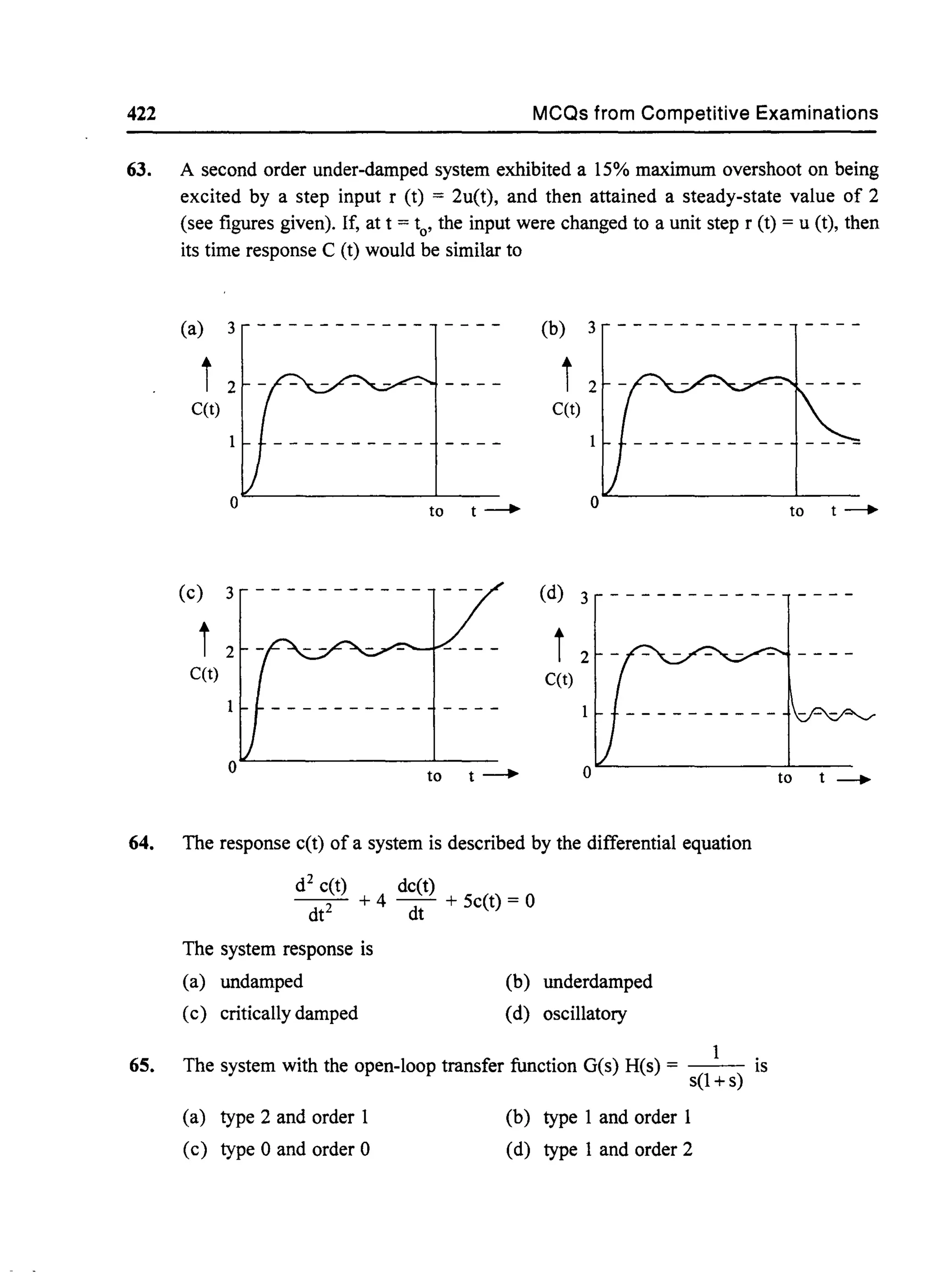
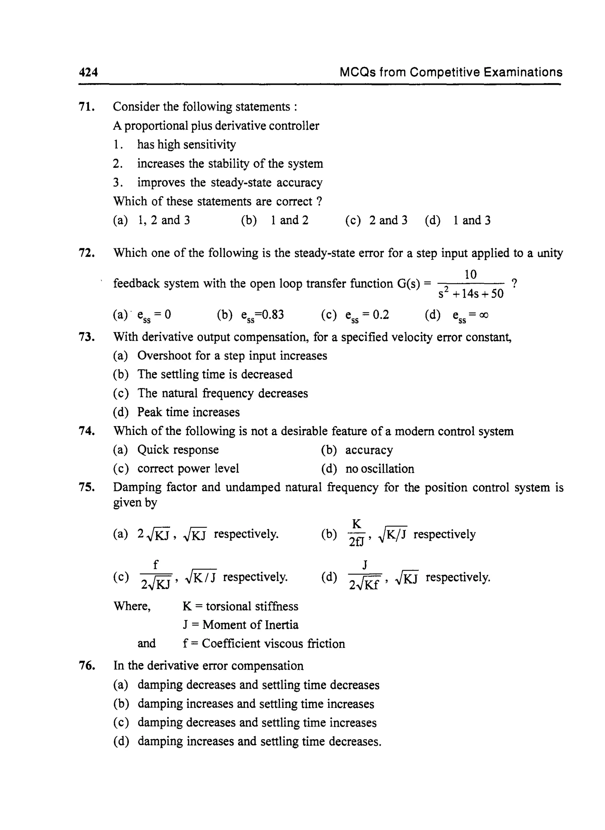
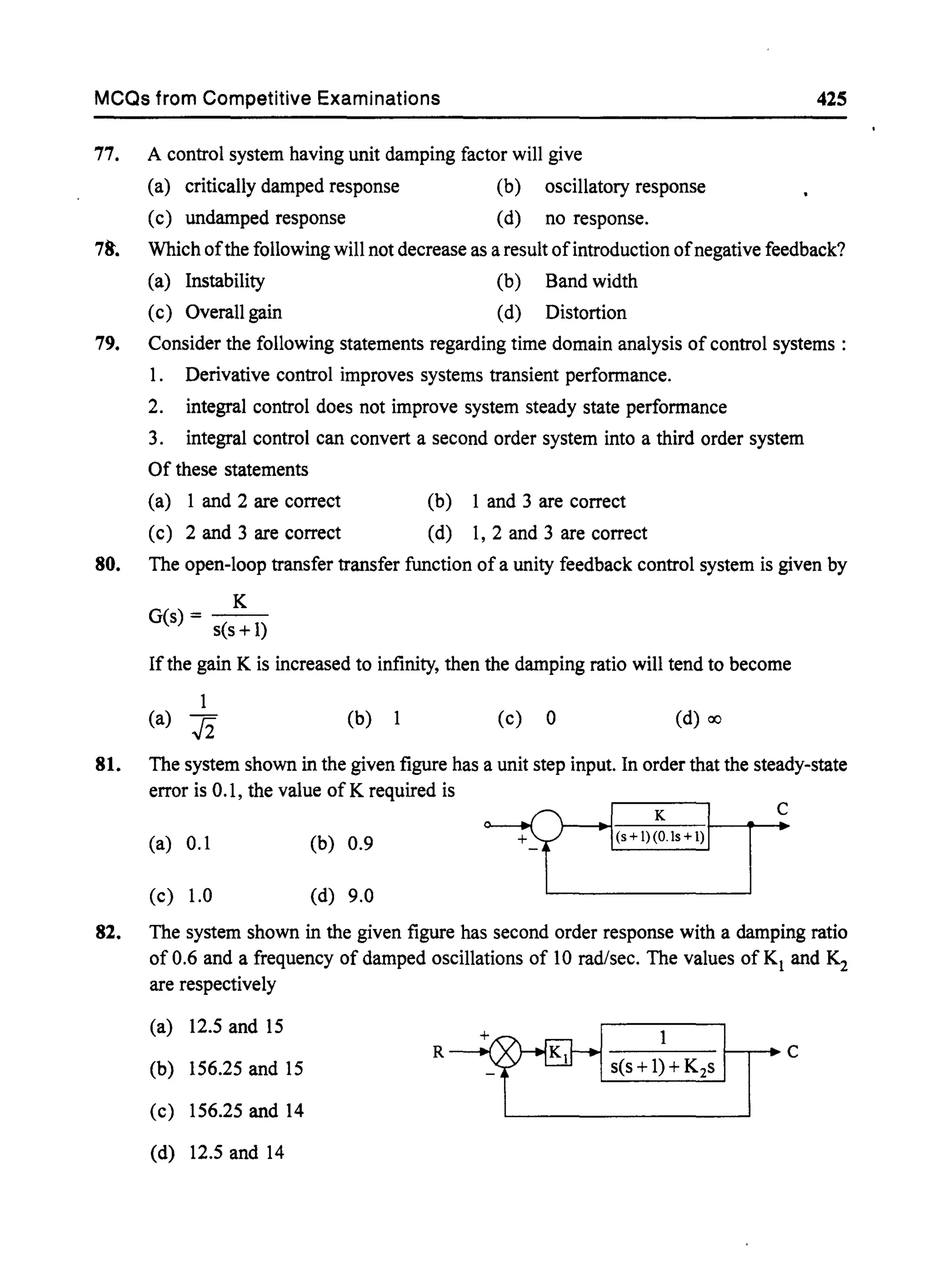
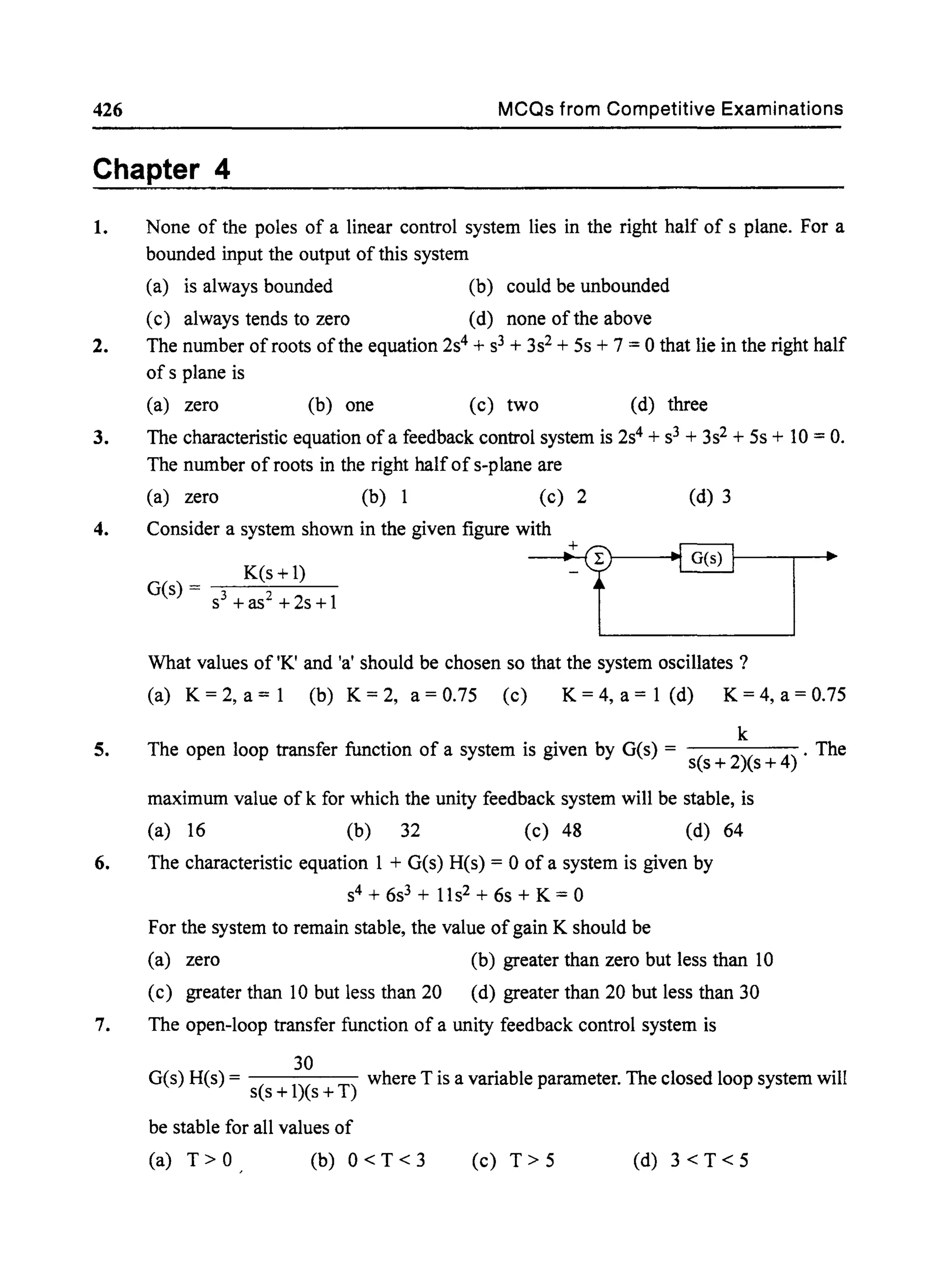
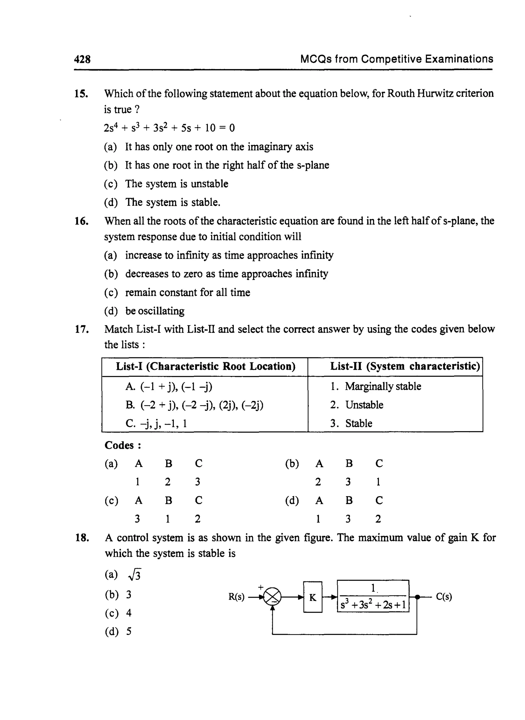
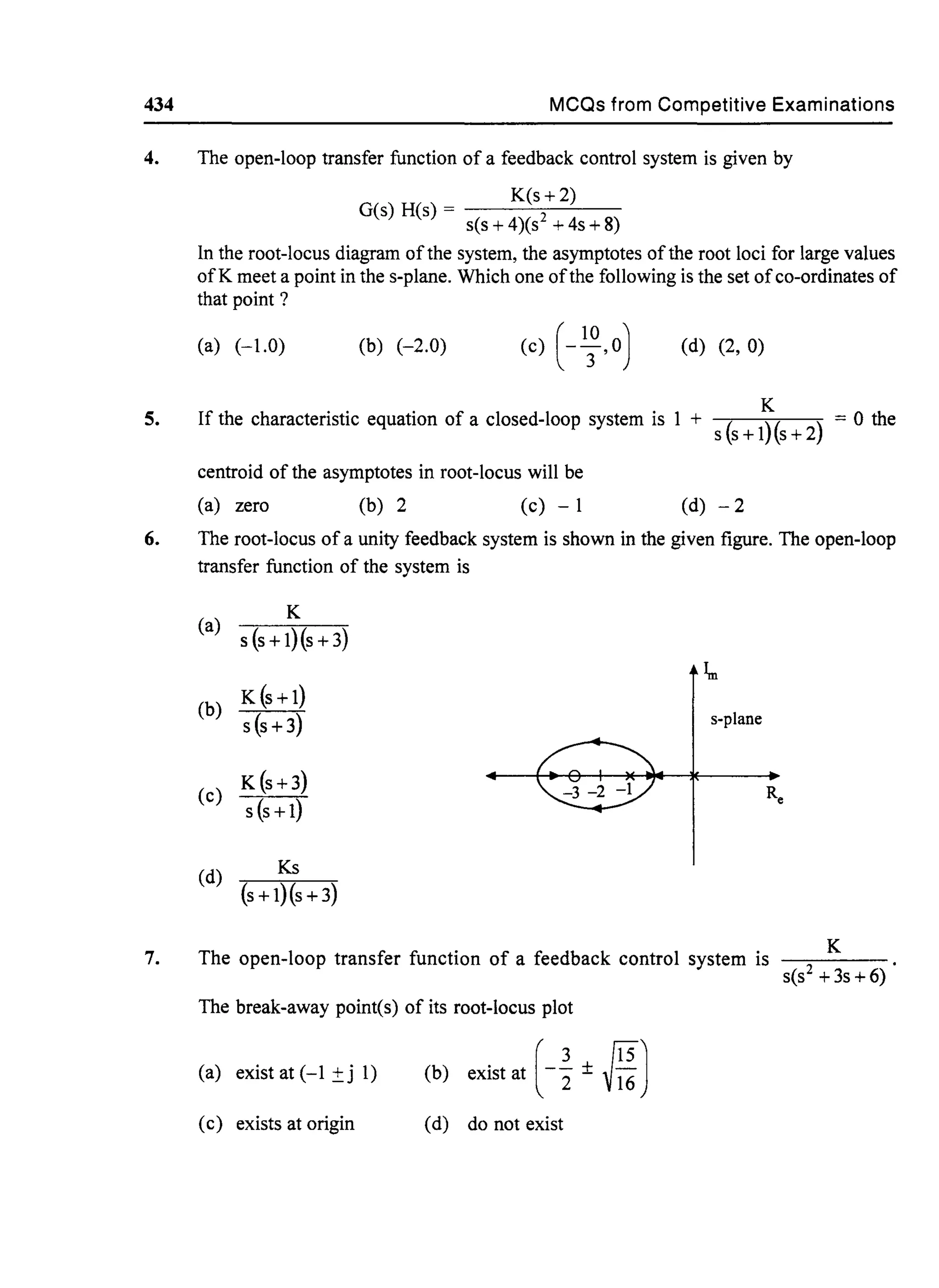
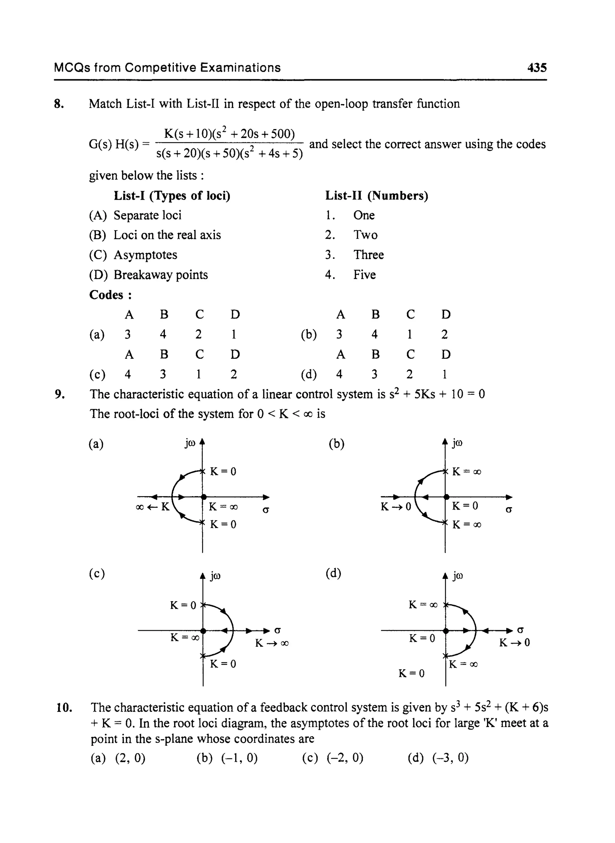
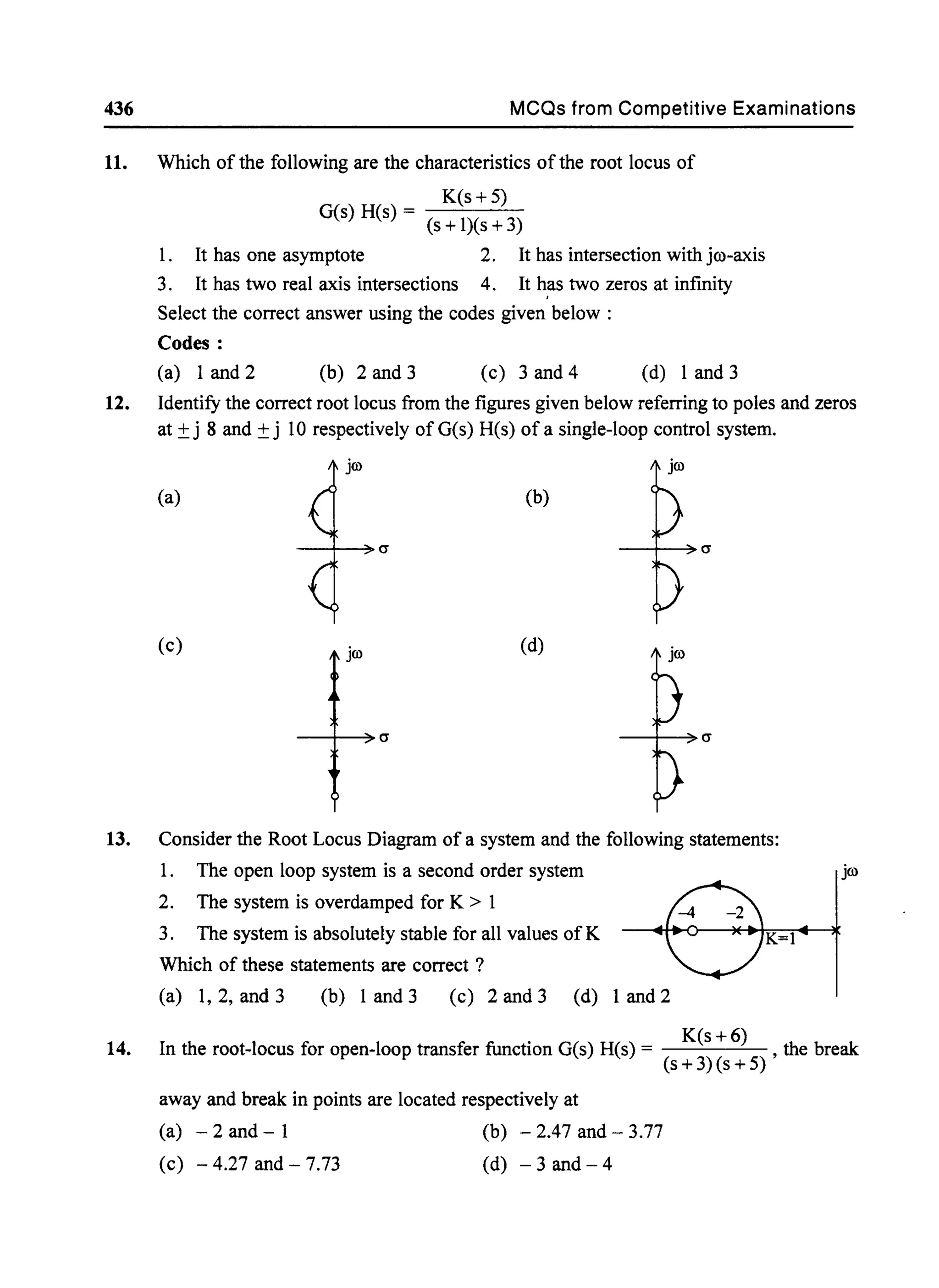
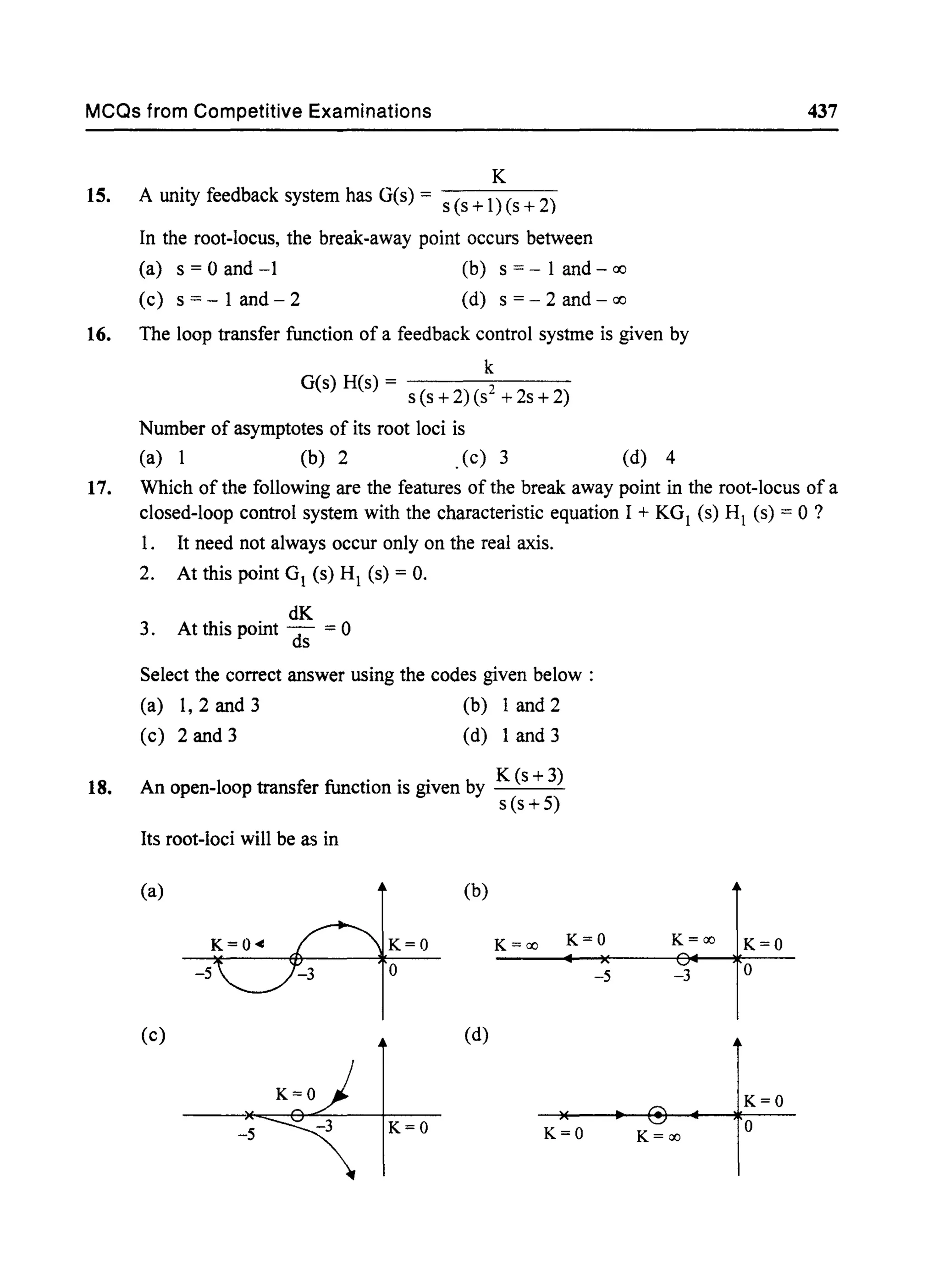
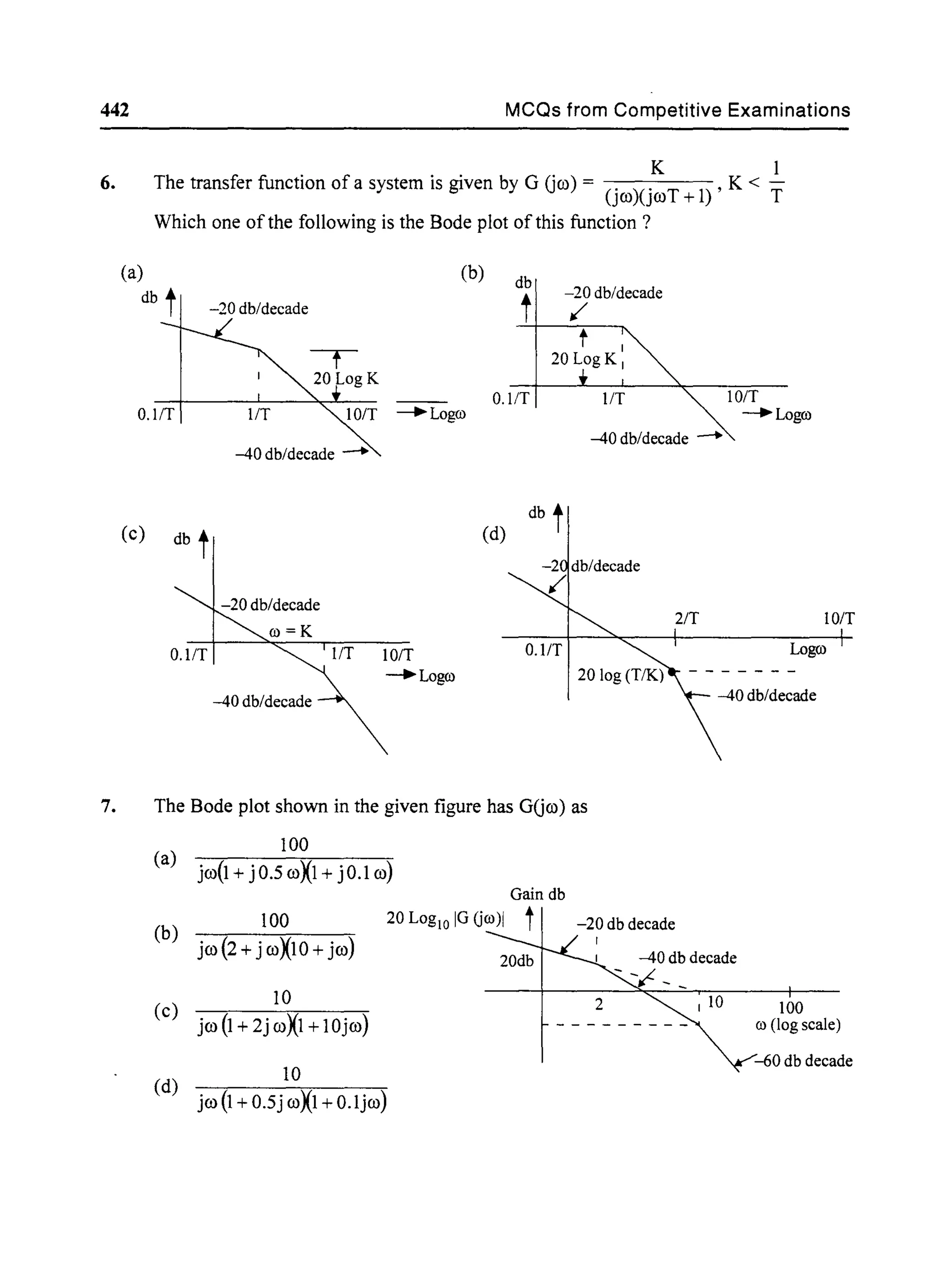
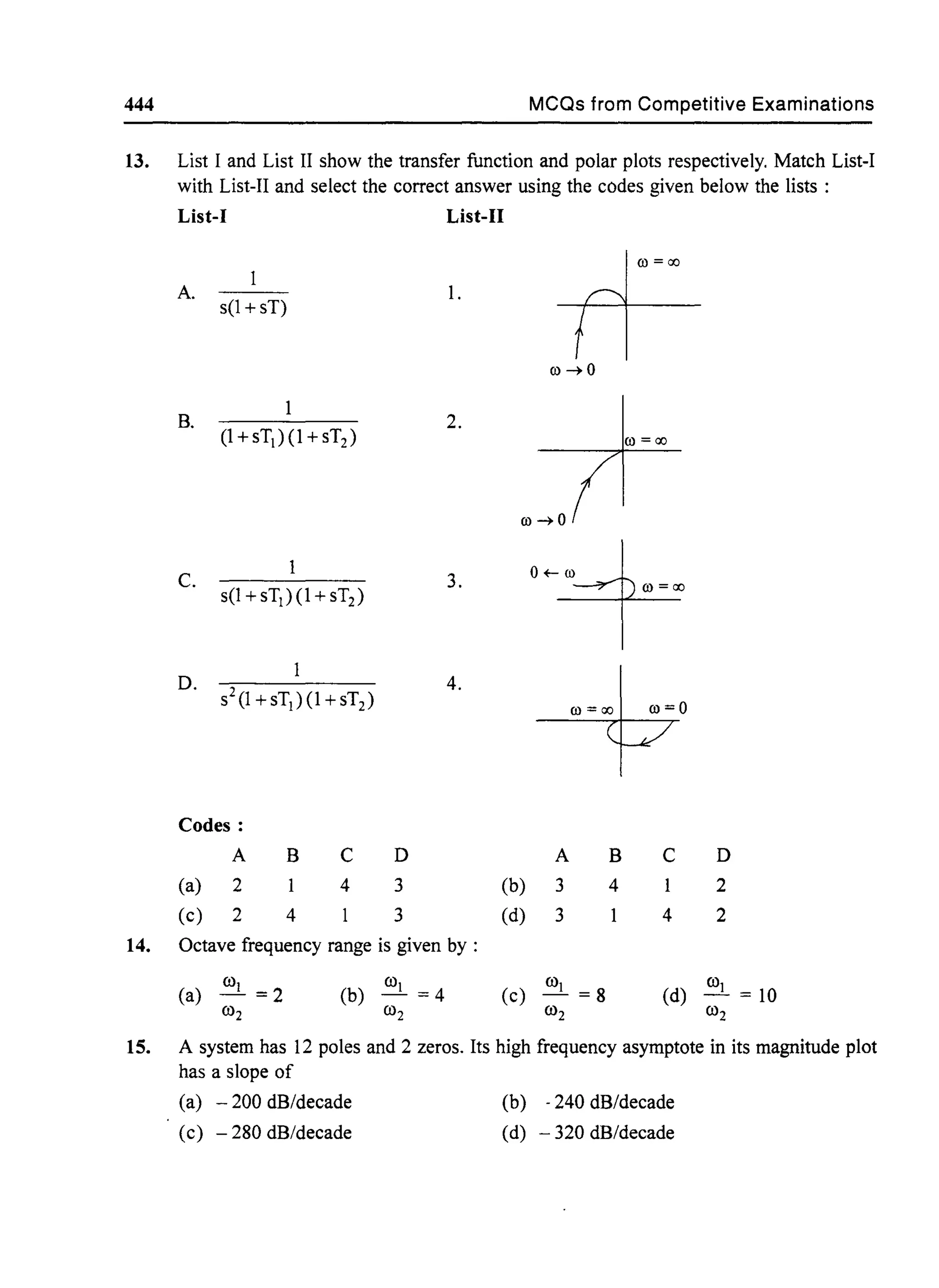
454. MCQs from Competitive Examinations
16. A linear stable time-invariant system is forced with an input x(t) = A sin rot
Under steady-state conditions, the output yet) of the system will be
17.
(a) A sin (rot + ~), where ~ = tan-1 IG Gro) I
(b) IG Gro) IA sin [rot + LG Gro)]
(c) I G Gro) IA sin [2 rot + LG Gro)]
(d) AG Gro) sin [rot + LG Gro)]
x(t) - - - - i
4
For the second-order transfer function T(s) = - - - -
S2 + 2s + 4
The maximum resonance peak will be
(a) 4
4
(b) -
3
(c) 2
G (s) f - - - - y(t)
2
(d) fj
445
18. The magnitude plot for a minimum phase function is shown in the figure. The phase
plot for this function.
(a) cannot be uniquely determined
(b) will be monotonically increasing from
00
to 1800
(c) will be monotonically decreasing from
1800
to 00
G.dB
+6dB/oct -6dB/oct
32dB --;~
12dB~ I I'"
I I I logro scale
0.1 0.5 1 5
(d) will be monotonically decreasing from 1800
to - 900
19. What is the slope change at ro = 10 of the magnitude vis frequency characteristic of a
unity feedback system with the following open-loop transfer function?
G(s) = 5(l+jO.lro)
jro (l + j 0.5 ro)[1 + j 0.6 (ro / 50) + Gro / 50)2]
(a) - 40 dB/dec to - 20 dB/dec
(c) - 20 dB/dec to - 40 dB/dec
(b) 40 dB/dec to 20 dB/dec
(d) 40 dB/dec to - 20 dB/dec

455. 446 MCQs from Competitive Examinations
20. Match List I with List II and select the correct answer using the codes given below the
lists:
List I (Transfer Functions) List II (Description)
1-s
A.
1+s
1. Non-minimum phase-system
1-s
B. (1 + s) (1 + 2s) (1 + 3s) 2. Minimum phase system
1+3s
C.
(1 + 4s)(1 + 2s)(1 + s)
3. All pass system
Codes: A B C
(a) 1 3 2
(b) 3 2 1
(c) 3 2
(d) 2 3
21. Which one ofthe following is the polar plot ofa typical type zero system with open-loop
transfer function G Gro) = k
(1 + jroT,)(l + jroT,)
(a)
(c)
-180°
-180°
Jf
GUm)
-270° (b)
-270° (d)
-90°
-270°
-180°
-270°

456. MCQs from Competitive Examinations
22.
23.
4
A second-order overall transfer function is given by - - - -
S2 +2s+4
Its resonant frequency is
(a) 2 (b) .J2 (c) J3 (d) 3
The phase angle for the transfer function G(s) = at corner frequency is
(l + sT)3
(a) - 45° (b) - 90° (c) - 135° (d) - 270°
447
24. The magnitude plot of a transfer function is shown in the figure. The transfer function
in question is
4(1+~) 4sl1 +~) Gain, dB
--6dB/octave
(a) (b)
--6dB/octave
S(l+ 1~) (
1
+ l~)
6dB
4(1+ 2s) 4s (1 + 2s) 2 10
(c)
s (1 + lOs)
(d)
(1 + lOs)
(02 (log scale)
25. The open-loop transfer function of a unity negative feedback system is
K (s + 10)(s + 20)
G(s) - --;:--------'--
- S3 (s+100)(s+200)
The polar plot of the system will be
(a)
ImG(s)
(b)
ReG(s)
(O=ao
ImG(s)
ReG(s)
(c) (d)
(O=ao
ImG(s)
ReG(s)
(O=ao
ImG(s)
(O=ao
ReG(s)
26. Open loop transfer function of a system having one zero with a positive real value is
called
(a) zero phase function (b) negative phase function
(c) positive phase function (d) non-minimum phase function

457. 448 MCQs from Competitive Examinations
27. An open loop transfer function of a unity feedback control system has two finite zeros,
two poles at origin and two pairs ofcomplex conjugate poles. The slope ofhigh frequency
asymptote in Bode magnitude plot will be
(a) + 40 dB/decade (b) 0 dB/decade
(c) .- 40 dB/decade (b) -80 dB/decade
28. A decade frequency range is specified by
(a) (02 = 2 (b) ~ = lU (c) ~ = 8 (d) none of the above
(01 (01 (01'
29. Which one of the following transfer functions represents the Bode plot shown in the
figure? IOdB
I-s .
(a) G= - 0) 1
l+s
(b) G= (1+S)2
1
(c) G = -
S2
1 -180°
(d) G = s(1 + s) -----0}-i=-1- - - - -
30. The characteristic equation of a closed-loop control system is given by s2 + 4s + 16 = 0
The resonant frequency in radians/sec of the system is
31.
(a) 2 (b) 2J3 (c) 4 (d) 2fi
The log-magnitude Bode plot of a minimum phase system is shown in the figure. Its
transfer function is given by
s-10
(a) G (s) = s+100
s+lO
(b) G (s) = s _ 100
s-10
(c) G (s) = s-100
s+lO
(d) G (s) = 's+100
o
N
20 - - - - - - -
8
0r-------~10~---80~~-----
100
32. For a closed-loop transfer function given below
C(s) 2600K(s + 25)
- - = the imaginary axis intercepts of the
R(s) S4 + 125s3
+ 5100s2
+ 65000s + 65000K
root loci will be
(a) ±j22.8 (b) ±j2.28 (c) ±j1.14 (d) ±j 11.4

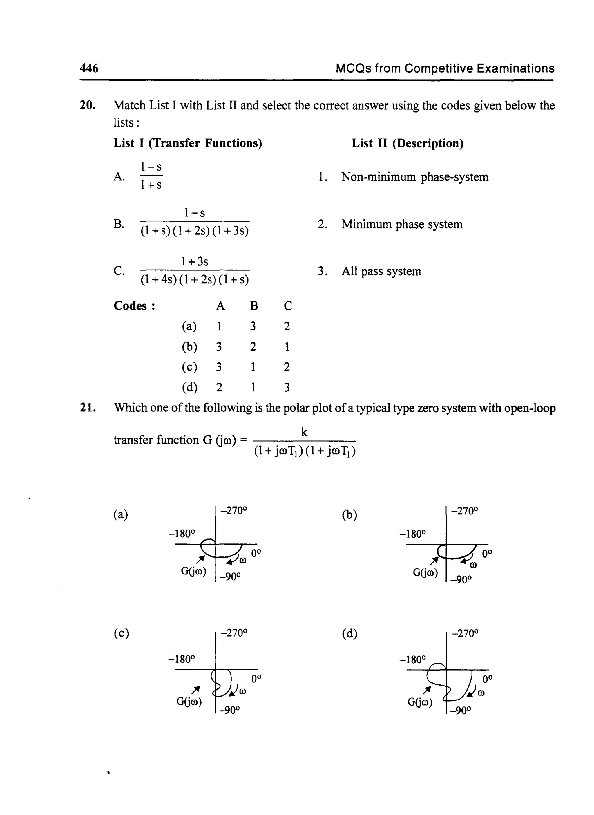
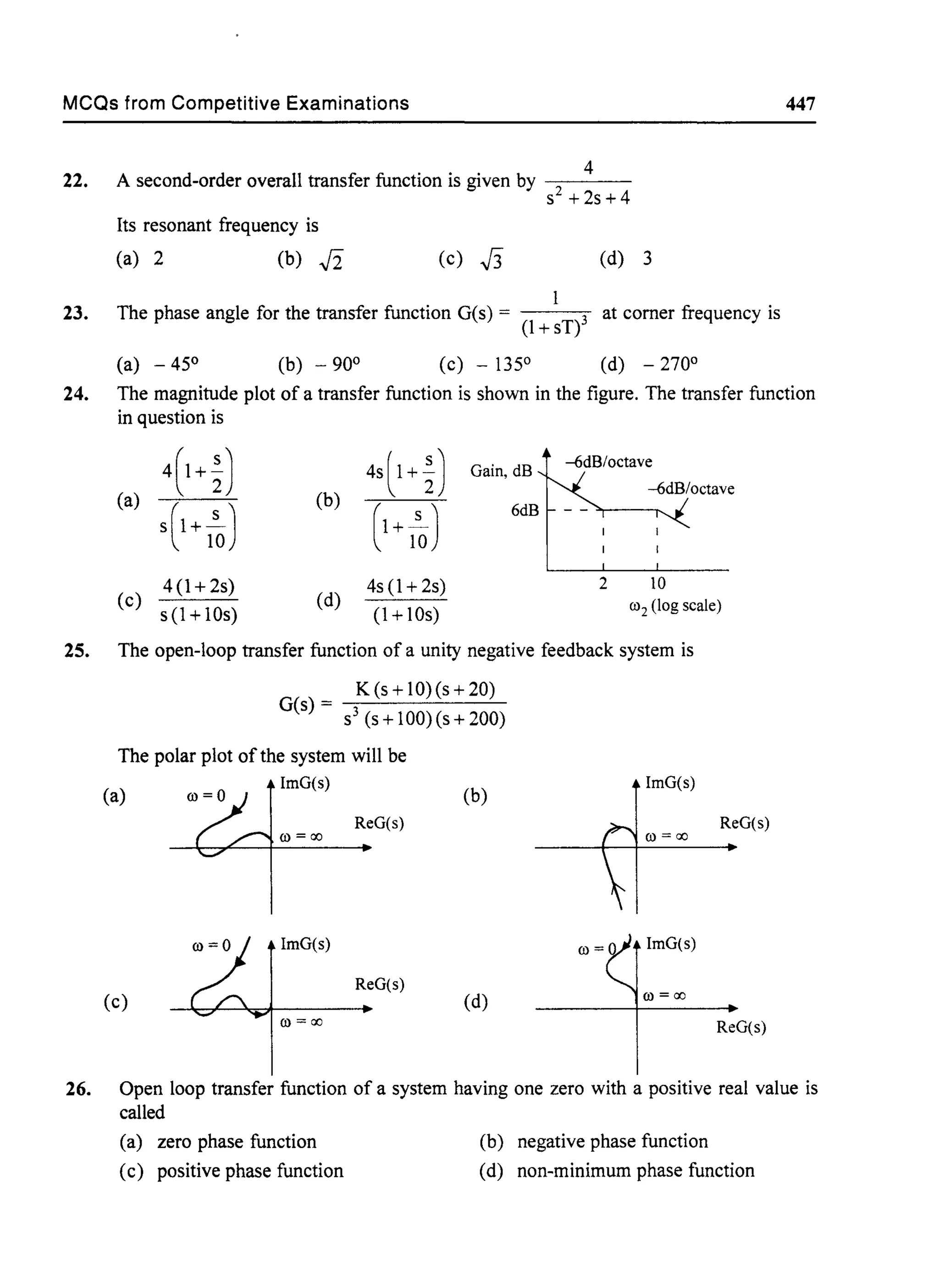
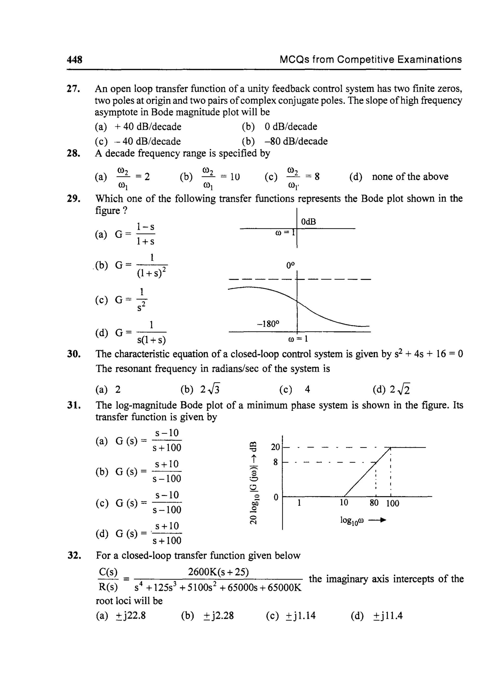
458. MCQs from Competitive Examinations 449
33. Match List I with List IT and select the correct answer using the codes given below the lists
A.
B.
c.
D.
List I [G(s) H(s)]
K
l+sTJ
K
(I + TlsXI + T2s)
K
s2(1 + sTI)
Codes:
(a) A B C
4 5
(c) A B C
4 2
2.
3.
4.
5.
D (b)
3
D (d)
3
List II (Nyquist plot)
r
0'
r
100
=00
•00 - 0 0'
b •00 -0 0'
ro=oo
~~~f~oo •0'00 = 0
A B C D
1 4 3 5
A B C D
4 2 5

459. 450 MCQs from Competitive Examinations
34. The Nyquist plot for a control system is shown in Figure. I. The Bode plot for the same
system will be as in
1m
(-1 +jO)
Nyquist plot (Figure 1)
(a)
-20 dB/dec
IGI 1---",,-
-40 dB/dec
--60 dB/dec
(c)
IGI
--60 dB/dec
Chapter 7
(b)
(d)
Re
IGI
:-40 dB/dec
-40 dB/dec
1. The polar plot of a type-I, 3-pole, open-loop system is shown in Fig. The closed-loop
system is
(a) always stable 1m G(s)
G(s)
(b) marginally stable
-1.42 Re G(s)
(c) unstable with one pole on the right half of s-plane
(d) unstable with two poles on the right half of s-plane

460. MCQs from Competitive Examinations 451
2. Which one ofthe following statements is true for gain margin and phase margin of two
closed-loop systems having loop transfer functions G(s) H(s)and exp(-s) G(s) H(s) ?
(a) Both gain and phase margins of the two systems will be identical
(b) Both gain and phae margins ofG(s) H(s) will be more
(c) Gain margins ofthe two system are the same but phase margin ofG(s) H(s) will be
more
(d) Phase margins ofthe two system are the same but gain margin ofG(s) H(s) will be
less
3. An effect of phase-lag compensation on servo system performance is that
(a) for a given relative stability, the velocity constant is increased
(b) for a given relative stability, the velocity constant is decreased
(c) the bandwidth of the system is increased
(d) the time response is made faster
4. If the compensated system shown has a phase margin of60° at the crossover frequency
of 1 rad/sec, the value of the gain k is
5.
(a) 0.366
(b) 0.732
(c) 2.738
(d) 1.366
C(s)
10
The open-loop transfer function of a unity feedback control system is 3 • The
(s +5)
gain margin of the system will be
(a) 20dB (b) 40dB (c) 60dB (d) 80 dB
6. The Nyquist plot of the open-loop transfer function. of a feedback control system is
shown in the given figure. Ifthe open-loop poles and zeros are all located in the left half
of s-plane, then the number of closed-loop poles in the right half of s-plane will be
Im
(a) zero
GH-plane
(b) ro=+CXl
Re
(c) 2
(d) 3

461. 452 MCQs from Competitive Examinations
7. Match List-I (Plot/diagram/chart) with List-II (Characteristics) and select the correct
answer using the codes given below the Lists :
List-J List-II
A. Constant M loci
B. Constant N loci
1.
2.
Constant gain and phase shift loci ofthe closed-loop system
Plot of loop gain with variation of co
C. Nichol's chart
D. Nyquist plot
3.
4.
Circles of constant gain for closed-loop transfer function
Circles ofconstant phase shaft ofclosed-loop transfer function
Codes:
(a) A
3
(c) A
4
B C
4 2
B._. C
3 2
D
I
D
(b) A
3
(d) A
4
B
4
B
3
C
I
C
D
2
D
2
8. Consider the Nyquist diagram for given KG(s) R(s). The transfer function KG(s) R(s)
has no poles and zeros in the right half of s-plane. Ifthe (-1, jO) point is located first in
'region I and then in region II, the change in stability of the system will be from
~
(a) unstable to stable
(b) stable to stable
(c) unstable to unstable
(d) stable to unstable
9. Consider the following Nyquist plots of different control systems:
Which of these plot(s) represent(s) a stable system?
Imaginary Imaginary
1. 2.
----r--+-
o:-----.Real
-1
-+-..-/----''1-
0
=----.Real
3. Imaginary 4. Imaginary
-+--'---:'1-
0
:-----'Real ---1--+--+-,0=---+ Real
-1
(a) 1 alone (b) 2,3 and 4 (c) 1,3and4 (d)1,2and4

462. MCQs from Competitive Examinations 453
10.
11.
12.
s
The transfer function of a certain system is given by G(s) = (1 +s)
The Nyquist plot of the system is
Im
0)=0
II'
Im
(a)
O)=~
---+-----+--~Re (b) -----+--------~----~Re
------."""'"-------------3>Re Re
(c) (d)
O)=ao
'"
10
The polar plot ofG (s) = 2 intersects real axis at 00 =000, Then, the real part and
s(s+l)
000 are respectively given by :
(a) -5, 1 (b) -2.5, 1 (c) -5, 0.5 (d) -5,2
For the transfer function G(s) H(s) = 1 the phase cross-over frequency is
s (s + 1) (s + 0.5)
(a) 0.5 rad/sec
(c) 1.732 rad/sec
(b) 0.707 rad/sec
(d) 2 rad/sec
13. The gain phase plot ofopen loop transfer function of four different systems labelled A,
B, C and °are shown in the figure. The correct sequence of the increasing order of
stability of the four systems will be Gain in dB' B A
(a) A, B, C, °
(b) 0, C, B,A
-270°
(c) B,A, 0, C
(d) B, C, D,A

463. 454
14.
MCQs from Competitive Examinations
For the gain-phase plot shown in the given figure, for the open-loop transfer function
G (s), gain margin, gain crossover frequency, phase margin and phase crossover
frequency are respectively
(a) 2 db, 100 rad/sec, 400 , 10 rad/sec
(b) 0 db, 10 rad/sec, - 400 , 100 rad/sec
(c) 2 db, 10 rad/sec, 400
, 100 rad/sec
(d) - 2 db, 10 rad/sec, - 400 , 100 rad/sec
IGI
db
o
-2
-270° -1800
LG
-140° -90°
15. The type and order of the system whose Nyquist-plot is shown in the given figure are
respectively 1m
(a) 0, 1
(b) 1,2 40
(c) 0,2
(d) 2, 1
O)~oo 0)=0
Re
16. A unity feedback system has the following open-loop frequency response:
ro IG Gro) I LI G Gro) I
2 7.5 - 1180
3 4.8 - 1300
4 3.15 - 1400
5 2.25 - 1500
6 1.70 - 1570
8 1.00 - 1700
10 0.64 - 1800
The gain margin and phase margin of the system are
(a) 0 dB, - 1700
(b) 3.86 dB, - 1800
(c) 0 dB, 100
(d) 3.86 dB, 100
17. The radius and the centre of M circles are given respectively by
(a) M~-l' [~~~l'ol M2 (-M )(b) M2 -1' M2 _1,0

464. MCQs from Competitive Examinations 455
18. For a given G(s) H(s) the complete polar plot is shown in the given figure. If all Ts are
positive, then how many poles of the closed-loop system will be there in the RHS ?
(a) zero
(b)
(c) 2
(d) 3
P=(-I,jO)
--- -----.
19. The polar plot ofthe open-loop transfer function ofa feedback control system intersects
the real exis at -2. The gain margin of the system is
(a) -SdB (b) OdB (c) -6dB (d) 40dB
20. Which one of the following statements regarding the stability of a feedback control
system is correct ?
(a) Gain margin (GM) gives complete information about the relative stability of the
system
(b) Phase margin (PM) gives complete information about the relative stability ofthe system
(c) GM and PM together gives information about the relative stability of the system
(d) Gain cross-over and phase cross-over frequencies give the required information
about the relative stability of the system.
21. The constant M loci plot is symmetrical with respect to
(a) real axis and imaginary axis
(b) M = 1 straight line and the real axis
(c) M = 1 straight line and the imaginary axis
(d) M = 1 straight line
22. The radius of constant-N circle for N = 1 is
(a) 2 (b) fi (c)
23. The constant M circle for M = I is the
1
(d) fi
( ) 'gh r Iastral t me x = - 2" (b) critical point (- I, jO)
(c) circle with r = 0.33 (d) circle with r = 0.67
24. The polar plot of a transfer function passes through the critical point (-1, 0). Gain
margin is
(a) zero (b) - 1 dB (c) 1dB (d) infinity

465. 456 MCQs from Competitive Examinations
25. The polar plbt (for positive frequencies) for the open-loop transfer function of a unity
feedback control system is shown in the given figure
26.
27.
28.
29.
The phase margin and the gain margin of the system are respectively
(a) 150° and 4 1m GUm)
jl
(b)
3 /
150° and - ,/ -0.25
4
,
-1
(c) 30° and 4 Re GUm)
3 "
(d) 30° and - -jl
4
Which one of the following features is NOT associated with Nichols chart ?
(a) (0 dB, - 180°) point on Nichols chart represents the critical point (-1 + jO)
(b) It is symmetric about -180°
(c) The M loci are centred about (0 dB, - 180°) point
(d) The frequency at the intersection of the G(jro) locus and M = +3 dB locus gives
bandwidth of the closed-loop system.
Which one of the following equations represents the constant magnitude locus in
G-plane for M = 1 ? {x-axis is Re G (jro) and y-axis is 1m G (jro)}
(a) x=-0.5 (b) x=O
(c) x2 + y2 = 1 (d) (x + Ii + y2 = 1
K
The open loop transfer function of a system is G(s) H(s) = - - - - - - -
(l + s) (l + 2s) (l +3s)
The phase crossover frequency roc is
(a) .J2 (b) (c) zero (d) fj
Nyquist plot shown in the given figure is a type
1m
(a) zero system
"(b) one system ",
I
Re
(c) two system
(d) three system

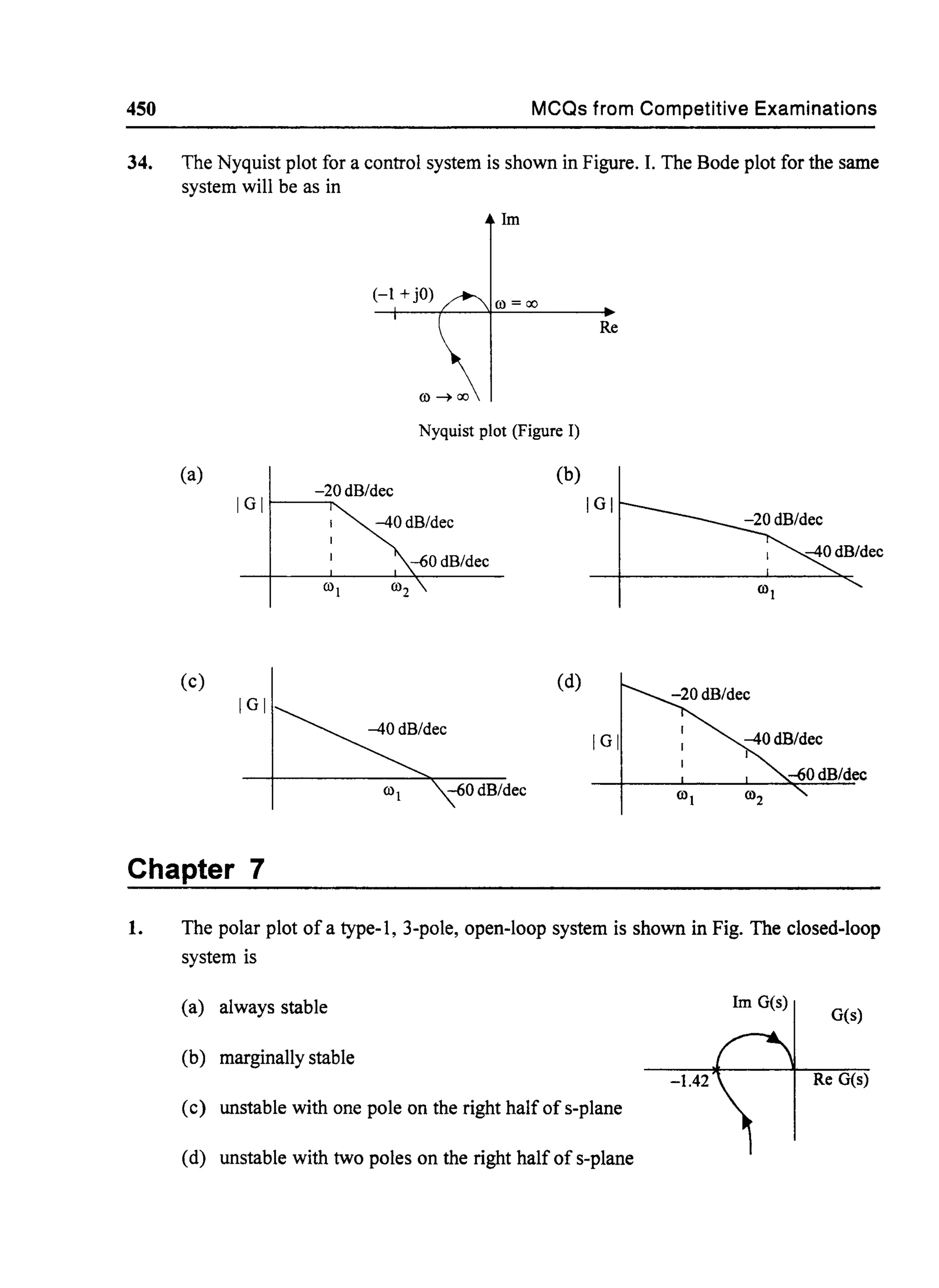
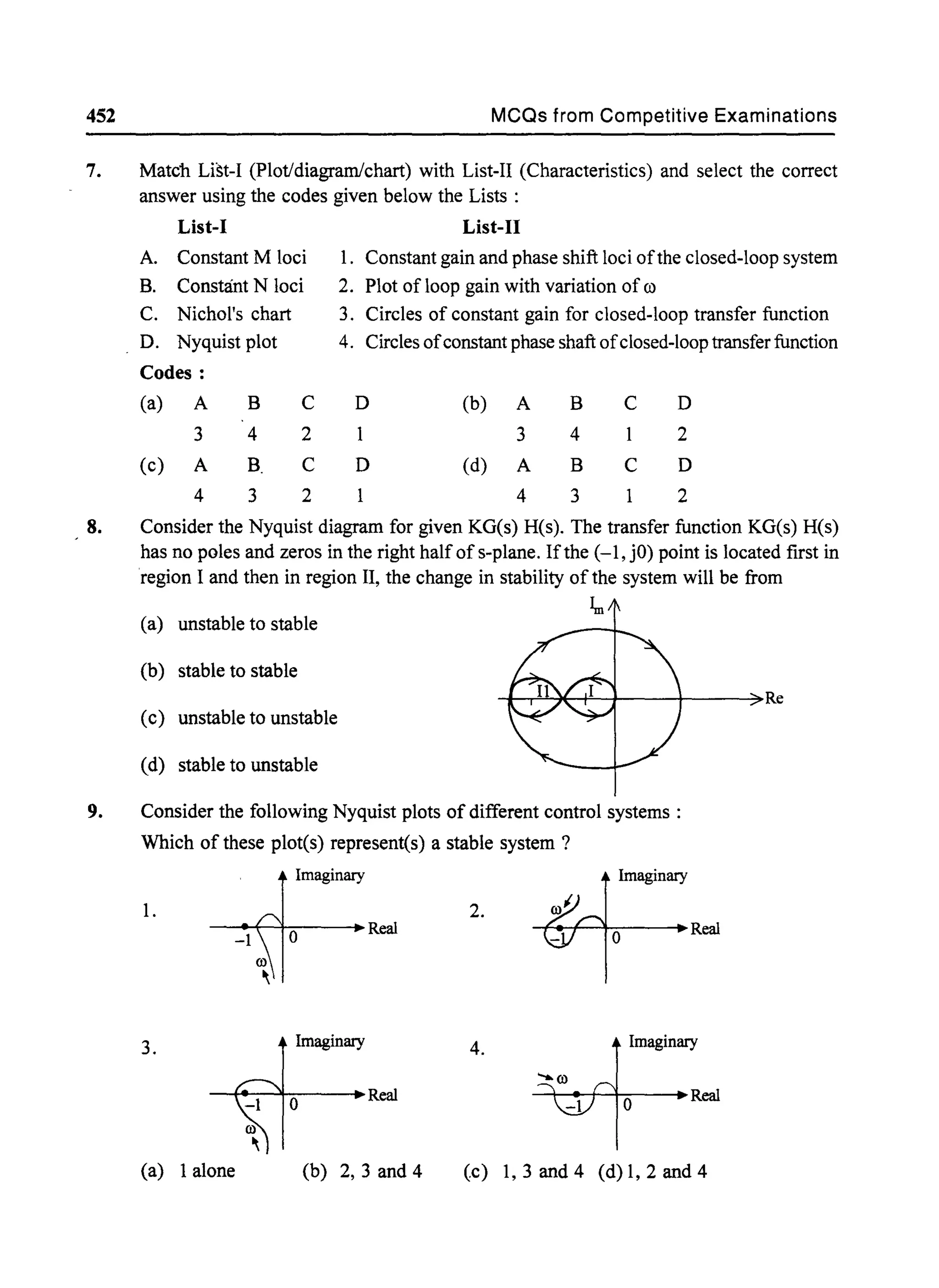
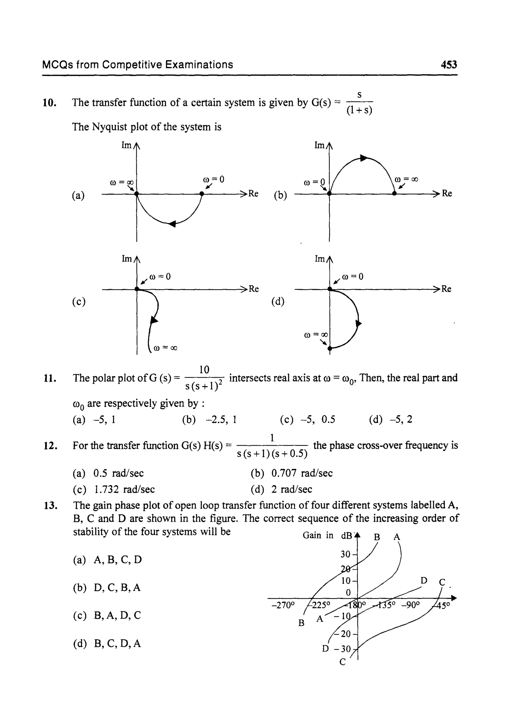
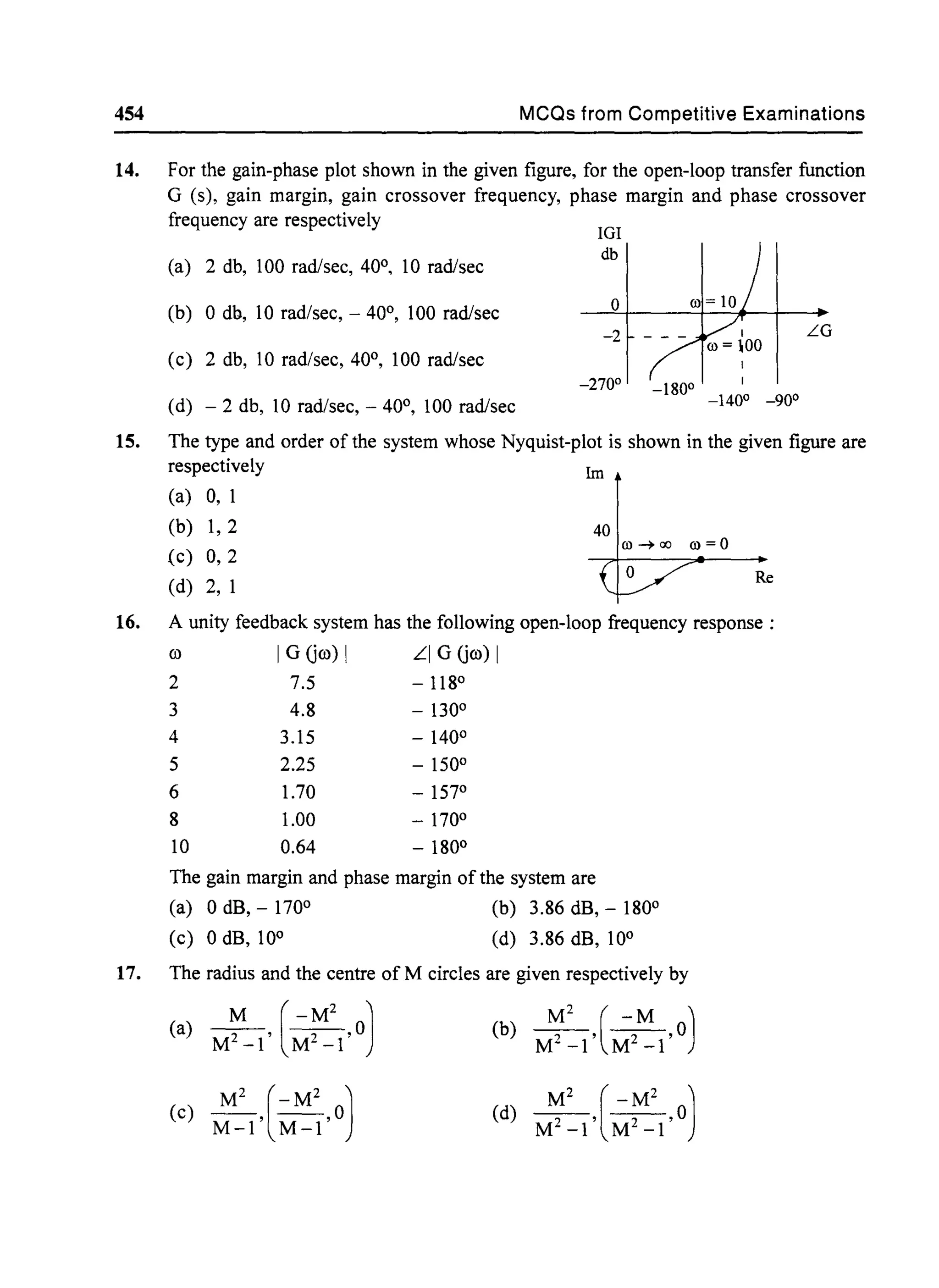
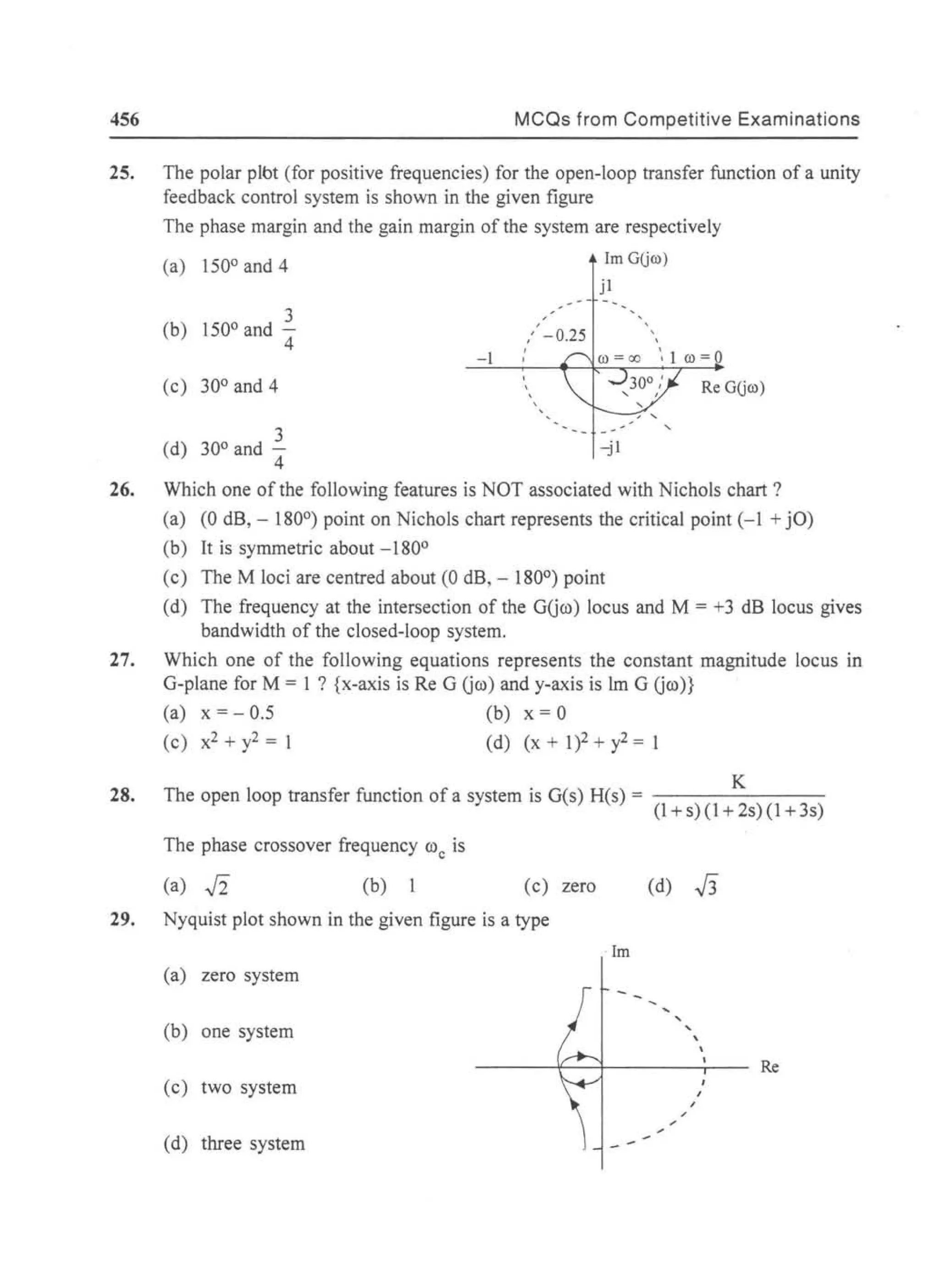
466. MCQs from Competitive Examinations 457
30. The open loop transfer function of a unity feedback control system is given as
1
31.
32.
33.
G(s) = s(l+sT)(1+sT2
)
The phase crossover frequency and the gain margin are, respectively,
I T + T2 T +T
(a) and TT (b) JTTz and ~T 2
JT T2 2 2
TT
(d) JTT2
and 2
T +T2
1
A constant N-circ1e having centre at (- "2 + jO) in the G-plane, represents the phase
angle equal to
(a) 180° (b) 90° (c) 45° (d) 0°
The constant M-circle represented by the equation x2 + 2.25x + y2 -= - 1.125 where
x = Re [G G(()] and y = 1m [G G(()] has the value of M equal to, ,
(a) 1 (b) 2 (c) 3 (d) 4
The advantages of Nyquist stability test ar~
(a) it guides in stabilising an unstable system
(b) it enables to predict closed loop stability from open loop results
(c) is is applicable to experimental results of frequency response of open loop system
(d) all ofthe above
34. The Nyquist locus of a transfer function G(s), H(s) = ~ is given in Fig. 1.
l+sT
1m 1m
())=oo ())=Q
--------r-- Re
K
Fig. I.
())=oo ())=Q
~~-----~~Re
K
Fig. II.
The locus is modified as shown is Fig. II on addition of pole or poles to the original
G(s) H(s) Then, the modified transfer function of the modified locus is
K
(a) G(s) H(s) = - - -
s(1 + sT)
(c) G(s) H(s) = ___K__
(1 + sT)(l + sT2)
(b) G(s) H(s) = _ _K_ _
(1 + sTj )(1 + sT2)
K
(d) G(s) H(s) = - - - - - - -
(1 + sT)(1 + sT2)(1 + sT3)

467. 458 MCQs from Competitive Examinations
35. The constant M-circ1es corresponding to the magnitude (M) of the closed-loop transfer
of linear system for values of M greater than one lie in the G-plane and to the
(a) right of the M = 1 line (b) left of the M = 1 line
(c) upper side of the M =+j 1 line (d) lower side of the m =-j 1 line
36. The Nyquist plot of servo system is shown in the Figure-I. The root loci for the system
would be
(a)
----------~~----~Re
Increasing
00
joo
Figure-I
(b)
joo
(c) (d) None of the drawn plot of (a), (b), (c) of
double pole
----~~--~~-----.cr
at origin
the question
37. Consider the following Nyquist plot of a open loop stable system:
The feedback system will be stable if and only ifthe critical point lies in the region
(a) I (OP)
00 < 0~~
(b) II (PQ)
N Real
(c) III (QR)
(d) None of these -
00 = 0+

468. MCQs from Competitive Examinations 459
Chapter 8
1. The gain cross-over frequency and bandwidth of a control system are IDeu and IDbu
respectively. A phase-lag network is employed for compensating the system. If the gain
cross-over frequency and band width of the compensated system are IDee and IDbe
respectively, then
(a) IDee < IDeu ; IDbe < IDbu
(c) IDee < IDeu ; IDbe > IDbu
(b) IDee> IDeu ; IDbe < IDbu
(d) IDee> IDeu ; IDbe > IDbu
2. A portion ofthe polar plot ofan open-loop transfer function is shown in the given figure
The phase margin and gain margin will be respectively
(a) 30° and 0.75
ImG(s)H(s)
, ,
(b) 60° and 0.375
,, ,
, ,
-0.75
(c) 60° and 0.375 -1
- 0.375
ReG(s)H(s)
1
,
(d) 60° and 0.75
3. If the transfer function of a phase lead compensator is s +a and that of a lag
s+b
compensator is s + p then which one of the following sets of conditions must be
s+q
satisfied?
(a) a> b and p > q
(c) a < b and p < q
(b) a > band p < q
(d) a < band p > q
4. The phase lead compensation is used to
5.
(a) increase rise time and decrease overshoot
(b) decrease both rise time and overshoot
(c) increase both rise time and overshoot
(d) decrease rise time and increase overshoot
(O.5s +1) .
Maximum phase-lead of the compensator O(s) = ( )' IS
0.05s +1
(a) 52 deg at 4 rad/sec
(c) 55 deg at 12 rad/sec
(b) 52 deg at 10 rad/sec
(d) None of the answer is correct

469. 460 MCQs from Competitive Examinations
6. Match List I with List II and select the correct answer using the codes given below the
lists:
List I List II
A. Transfer function of a lag network l. L-I (51 - Atl
B. State-transition matrix for X = AX 2.
(s + Z) Z
(s + P)' P > 1
C. DC amplifier transfer function 3. k
D. Steady state error of type-l system for step input 4. L-I (sA - 1)-1
5.
s+z z
-- , - < 1
s+p P
6. K(1 + sT)
7. zero
8. ao
Codes: A B C D
(a) 1 3 4 5
(b) 2 3 1 8
(c) 5 4 6 8
•(d) 2 3 7
7. Match List-I with List-II and select the correct answer using the codes given below the
lists:
List-I List-II
A. Phase lag controller 1. Improvement in transient response
B. Addition ofzero at origin 2. Reduction in steady-state error
C. Derivative output compensation 3. Reduction in settling time
D. Derivative error compensation 4. Increase in damping constant.
Codes:
A B C D
(a) 4 3 2
(b) 2 3 4
(c) 4 3 2
(d) 2 3 4

470. MCQs from Competitive Examinations 461
8.
10(1+.04s)
A phase-lead compensator has the transfer function Gc(s) = (l + .01s)
The maximum phase-angle lead provided by this compensator will occur at a frequency
rom equal to
(a) 50 rad/sec (b) 25 rad/sec (c) 10 rad/sec (d) 4 rad/sec
9. Match List I with List II and select the correct answer using codes given below the lists:
List I (Circuit diagram) List II (Name)
A.
:rWlv~
~ : l. Lag network
0 WIv
B.
I
0
2. Lead network
0 =r: 0
o----j~
+:fc. 3. Lag-lead network
0
0 c!J 0
iD. 4. Lead-lag network
0 -r 0
Codes:
(a) A B C D (b) A B C D
2 3 4 2 3 4
(c) A B C D (d) A B C D
2 4 3 2 4 3

471. 462 MCQs from Competitive Examinations
10. The root-locus plot for an uncompensated unstable system is shown in the given figure.
11.
The system is to be compensated by a compensating zero. The most desirable location
of the compensating zero would be the point marked,
(a) A
(b) B
(c) C
(d) 0
A· B C
1+ O.l2s
The transfer function of a lead conpensator is Ge(s) = 00
1+ . 4s
D
The maximum phase shift that can be obtained from this compensator is
(a) 60° (b) 45° (c) 30° (d) 15°
12. The transfer function ofa phase lead compensator is given by 1+ aTs where a > I and
I+Ts
T> O. The maximum phase shift provided by such a compensator is
(a) tan-l - - (b) tan-l - - (c) sm-l - - (d) sm-l - -
(
a+l) (a-I). (a+l) . (a-I)
a-I a+1 a-I a+1
13. Indicate which one ofthe following transfer functions represents phase lead compensator?
s+1
(a) -
s+2
(b) 6s+3
6s+2
(c) s+5
3s+2
(d) s +8
s2+5s+6
14. The maximum phase shift that can be provided by a lead compensator with transfer
15.
I +6s
function, G (s) = 1+ 2s
(a) 15° (b) 30° (c) 45° (d) 60°
1+0. Ts
The transfer function of a compensating network is of the form - - -
(1 +Ts)
If this is a phase-lag network the value of a. should be
(a) exactly equal to 0 (b) between 0 and I
(c) exactly equtal to I (d) greater than I

472. MCQs from Competitive Examinations 463
16. For the given phase-lead network, the maximum possible phase lead is
(a) sin-1 (1/3) IF
(b) 30°
~ :~wn(c) 45°
(d) 60°
17. When phase-lag compensation is used in a system, gain crossover frequency, band
width and undamped frequency are respectively
(a) increased, increased, increased (b) increased, increased, decreased
(c) increased, decreased, decreased (d) decreased, decreased, decreased
18. A lag compensator is basically a
(a) high pass filter (b) band pass filter
(c) low pass filter (d) band elimination filter
19. Which one of the following is a phase-lead compensation network?
(a) O_-----'cC-J~--"----.--_O (b)
[
o..--_-.l..-f~o
(c) (d)
O_________________l[L-__-OO
1
s+-
20. The phase-lead network function Gc (s) = -t, where a < 1 would provide
maximum phase-lead at a frequency of
1
(a) -
T
1
(b) -
aT
s+-
1
(c) -
T.Ja
aT
1
(d) -
aJT

473. 464 MCQs from Competitive Examinations
21.
5 (1 + O.3s)
The compensator G (s) = ---'----'-- would provide a maximum phase shift of
c 1+0.ls
(a) 20° (b) 30° (c) 45° (d) 60°
22. For the given network, the maximum phase lead ~m ofVo with respect to Vi is
(a) sin-1
(~J2R2
Rj
(b) sin-1 ( R
j
)
r
C~
!R2
1
R j +2R2
Cj
(c) sin-1
(R j :~RJ
(d) sin-1
(2~jCJ
23. The transfer function of a phase lead network can be written as
24.
(a)
l+sT
~ > 1 (b)
a (1 +sT)
1+ s~T ' l+saT
, a<1
(c)
~(1 +sT) .
~ < 1 (d)
(1 + sT)
a>1
l+s~+T ' a(l+saT) ,
Which one ofthe following compensations is adopted for improving transient response
of a negative unity feedback system ?
(a) Phase lead compensation
(b) Phase lag compensation
(c) Gain compensation
(d) Both phase lag compensation and gain compensation
25. For a given gain constant K, the phase-lead compensator
(a) reduces the slope of the magnitude curve in the entire range of frequency
(b) decreases the gain cross-over frequency
(c) reduces the phase margin
(d) reduces the resonance peak Mp

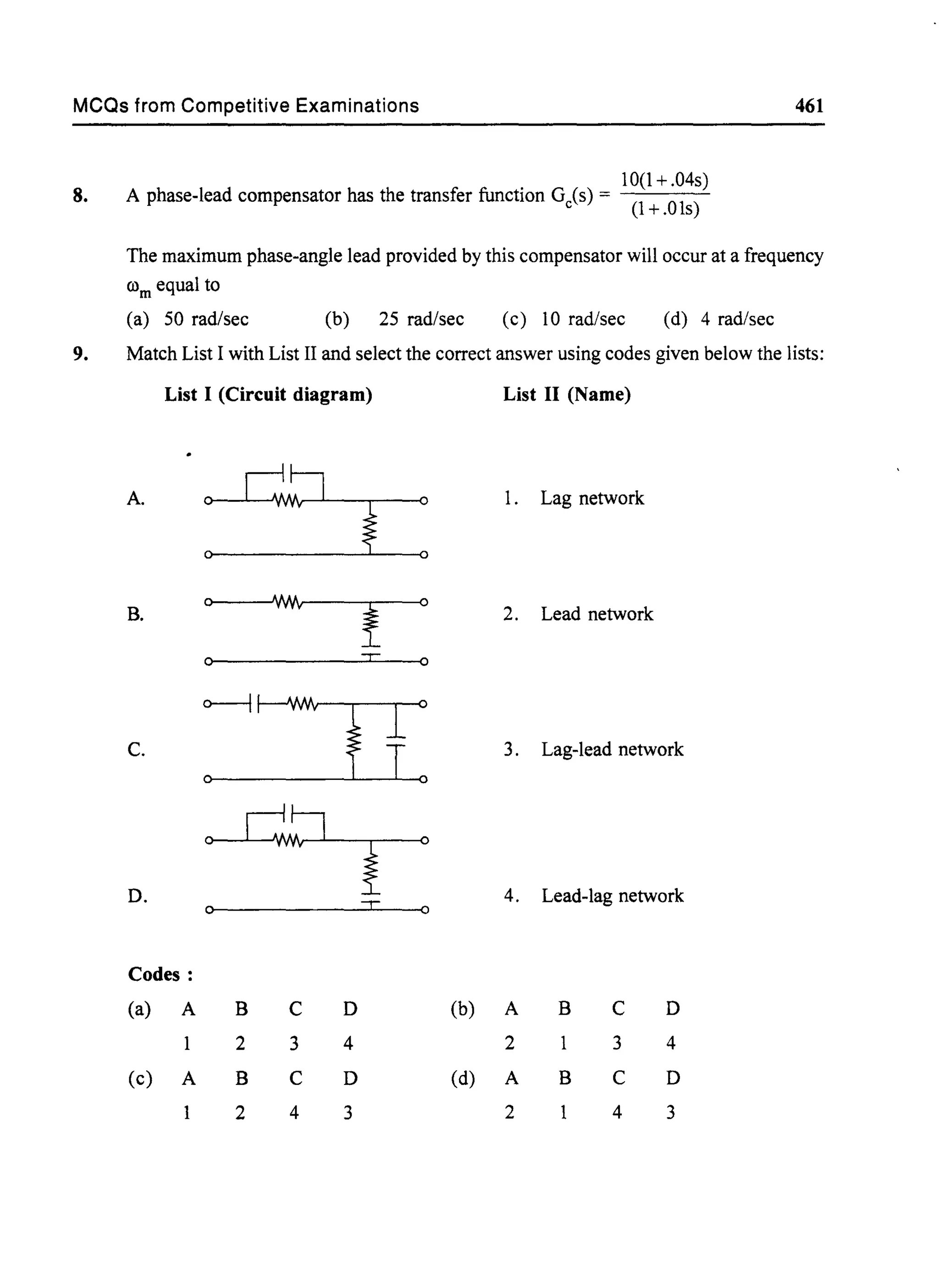
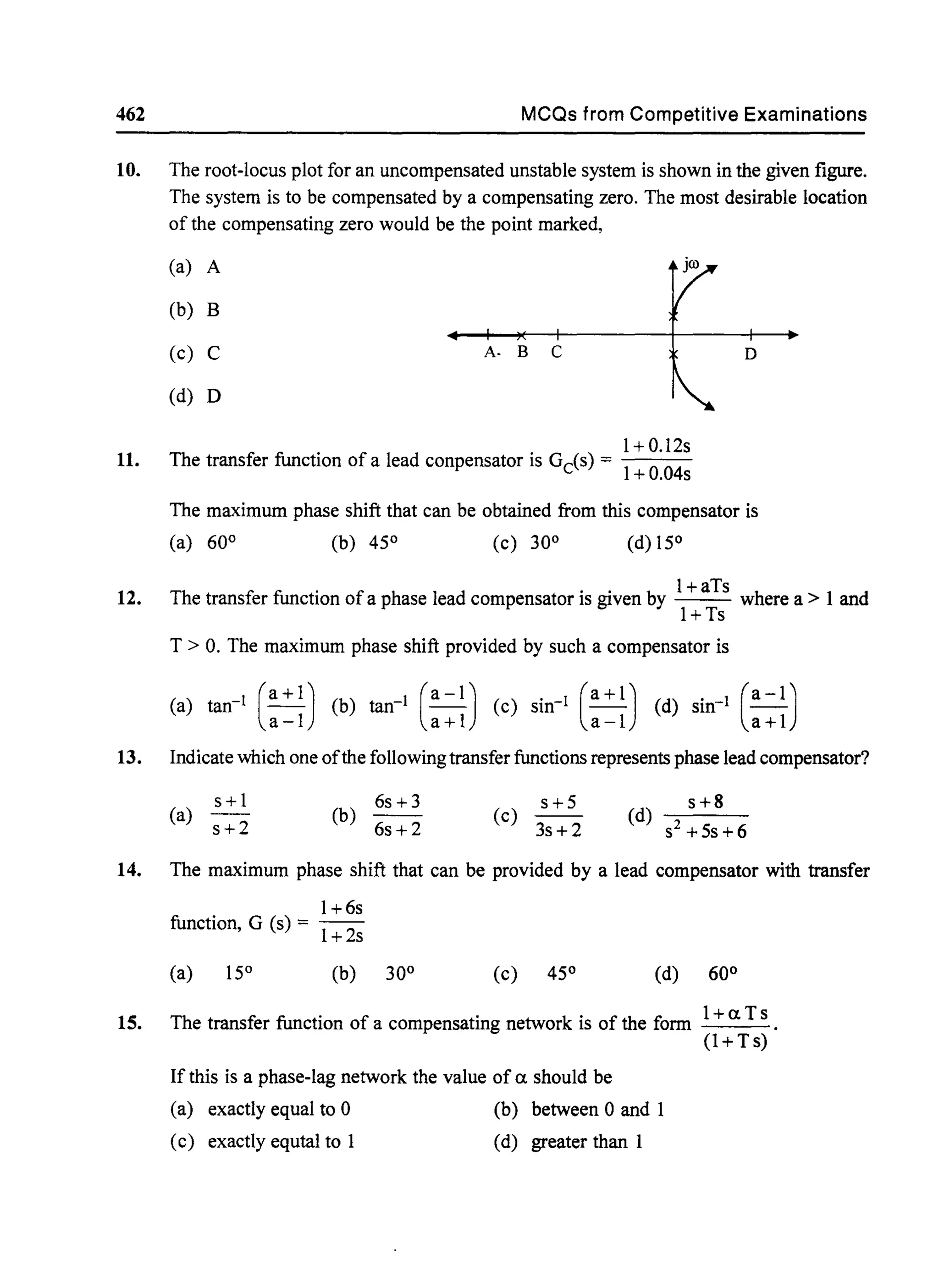
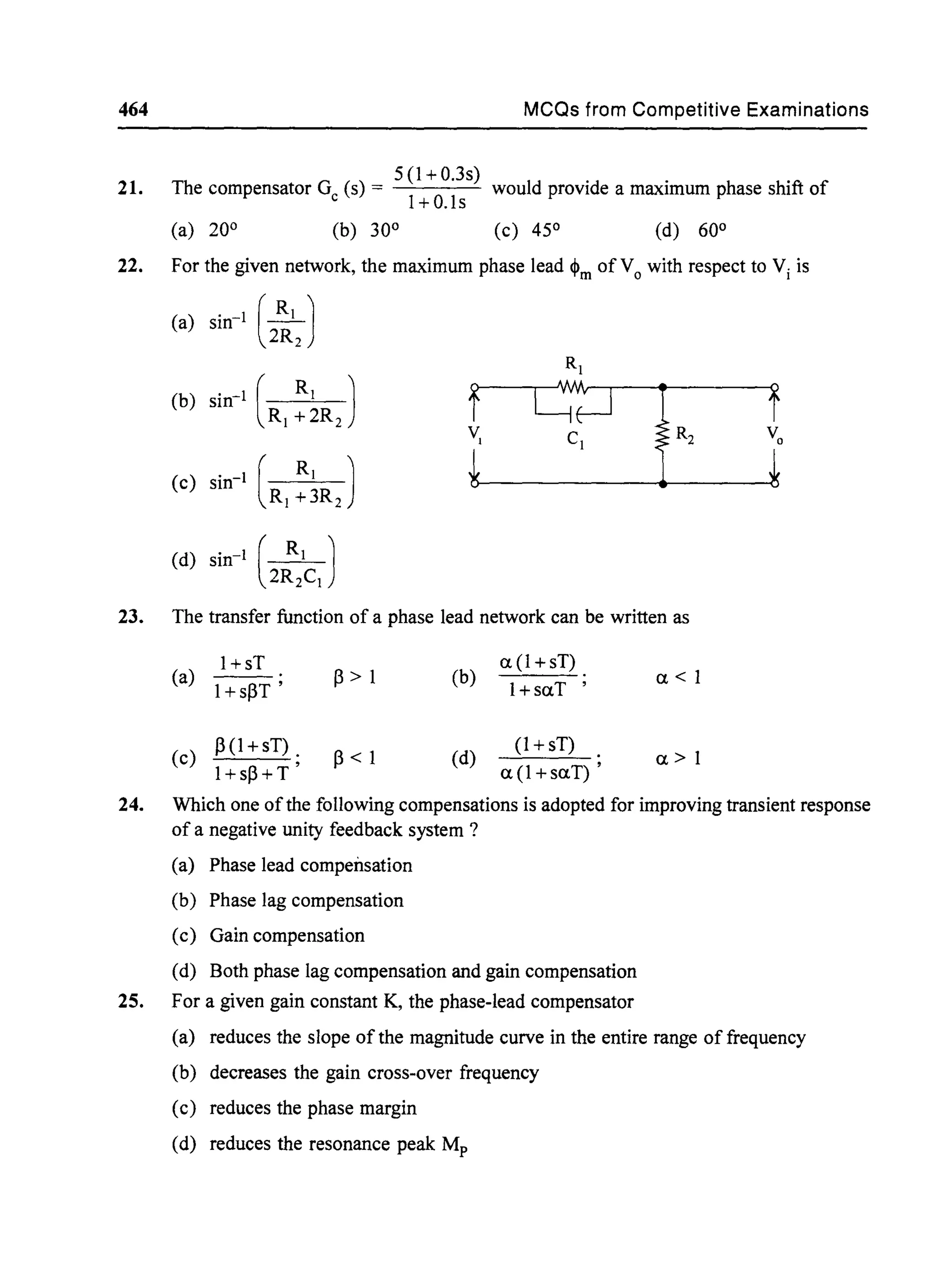
474. MCQs from Competitive Examinations
26. Consider the following statements:
In a feedback control system, lead compensator
1. increases the margin of stability
2. speeds up transient response
3. does not affect the system error constant
Of these statements
(a) 2 and 3 are correct (b) 1 and 2 are correct
(c) 1 and 3 are correct (d) 1, 2 and 3 are correct
27. A phase-lag compenstion will
28.
(a) improve relative stability
(c) increase bandwidth
(b) increase the speed of response
(d) increase overshoot
. 4(1+0.15s)
Maxlmum phase lead of is equal to
(l + 0.05s)
(a) 15° (b) 30° (c) 45° (d) 60°
Chapter 9
1. The state transition matrix for the system X = AX with initial state X (0) is
(a) (sl - Atl
(b) eAt X (0)
(c) Laplace inverse of [(sl - Atl]
(d) Laplace inverse of [(sl - Atl X (0)]
465
2. For the system X = [~ ~] X + [~] u; y = [4 0] X, with u as unit impulse and with
3.
zero initial state the output, y becomes :
(a) 2e2t (b) 4e2t (c) 2e4t
. ° °The eigenvalues of the system represented by X =
[
0 1
° °
° °(a) 0,0,0,0 (b) 1,1,1,1 (c) 0,0,0,-1
(d) 4e4t
(d) 1,0,0,0

475. 466 MCQs from Competitive Examinations
4. Given the homogeneous state-space equation X = [- 3 1] X the steady state value
° -2
5.
ofxss = lim x (t), given the initial state value ofx (0) = [10t~<X)
-lOf, is
(a) xss = [~] [
-10]
(c) -10
Consider the system X(t) = [~ ~] X(t) + [::J U(t); y (t) = [dl d2] X (t)
The conditions for complete state controllability and complete observability is
(a) dl =1= 0, b2 =1= 0, bi and d2
can be anything
(b) dl > 0, d2 > 0, bi
and b2
can be anything
(c) bi =1= 0, b2 =1= 0, dl and dz can be anything
(d) bi
> 0, b2
> 0, b2
and dl
can be anything
6. The transfer function of a multi-input multi-output system, with the state-space
representation of
X =AX+BU Y=CX+DU
where X represents the state, Y the output and U the input vector, will be given by
(a) C(sI _Ati B (b) C(sI -Atl B + 0
(c) (sl - Ati B + 0 (d) (sl _Ati B + 0
7. The state variable description of a single-input single-output linear system is given by
K = A X(t) + Q u (t)
yet) = £ X (t)
where A = G~lb = [~] and c = [1, -1]
The system is
(a) controllable and observable
(b) controllable but unobservable
(c) uncontrollable but observable
(d) uncontrollble and unobservable

476. MCQs from Competitive Examinations 467
8. Which ofthe following properties are associated with the state transition matrix ~ (t) ?
1. ~ (-t) = ~-l (t) 2. ~ (t/t2) = ~ (t1). ~-l (t2)
3. ~ (t1 - tz) = ~ (-t2)· ~ (t1)
Select the correct answer using the codes given below :
Codes:
(a) 1, 2 and 3 (b) 1 and 2 (c) 2 and 3 (d) I and 3
9. The second order system X = AX has A = [~I ~I]
The values of its damping factor 1; and natural frequency ron are respectively
(a) I and I (b) 0.5 and I (c) 0.707 and 2 (d) I and 2
10. A liner system is described by the state equations, [:J= [~ ~] [:J+ [~] r
c = Xz
Where r and c are the input and output respectively. The transfer function is :
(a) 1 /(s + 1) (b) 1 /(s + 1)2 (c) 1 /(s - 1) (d) 1 /(s - 1)2
11. The transfer function of a certain system is Yes) = 4 3 2 .
U(s) s +5s +7s +6s+3
The A,.e. matrix pair ofthe equivalent state-space model will be
[I
1 0
jJ[;1 [i3
1 0
jJ[;1
0 1 0 1
(a)
0 0
(b)
0 0
-6 -7 -5 -6
[I
1 0
jJ[~I [J3
0 0
II [~I
0 1 1 0
(c)
0 0
(d)
0
-7 -6 -6 -7

477. 468 MCQs from Competitive Examinations
12. The state equation of a dynamic system is given by X(t) = A X(t)
-1 1 0 0 0
0 -1 0 0
A= 0 0 -1 0 0
0 0 0 -3 4
0 0 0 -4 -3
The eigen values of the system would be
(a) real non-repeated only (b) real non-repeated and complex
(c) real repeated (d) real repeated and complex
13. The value ofA matrix in X = AX for the system described by the differential equation
y + 2 y + 3y = 0 form is
14. The state and output equations of a system are as under:
[
XI (t)] [0 1] [XI(t)] [0]State equation:. = + u(t)
x2(t) -1 - 2 x2 (t) 1
[
XI (t)]Output equation: C (t) = [1 1] X2(t)
The system is
(a) neither state controllable nor output controllable
(b) state controllable but not output controllable
(c) output controllable but not state controllable
(d) both state controllable and output controllable
15. The minimum number of states necessary to describe the network shown in the figure
in a state variable form is
(a) 2
50 lllF lOmH
0
~I
I
(b) 3
In In
(c) 4
51lF
(d) 6

478. MCQs from Competitive Examinations 469
16. A system is represented by y + 2 Y+ 5 y + 6y = 5x
If state variables are xl = y, x2 = y and x3 = y, then the coefficient matrix 'A' will be
[
0 I 0] [0 I 0] [0(a) ° ° I (b) ° ° I (c) °-6 -5 -2 -2 -5 -6 -6
~ ~1(d) [~ ° ~1-5 -2 -2 -5 -6
17. The state equation ofa linear system is given by X = AX + BU, where
A = [_02 ~] and B = [~]
The state transition matrix of the system is
(aJ [e;' e~'1 [
sin 2t cos 2t] [ cos 2t sin 2t]
(c) _ cos 2t sin 2t (d) - sin 2t cos 2t
18. The control system shown in the given figure is represented by the equation
[Yl(S)] = [Mat~ 'G'] [Ul(S)]
Y2(S) u2(s)
The matrix G is
(aJ [! -ll ~J [! ~~l
(c) [(,:1) (S~I)21 (d) [(S:I) -(S~IY
° ° ---(s+l) (s+l)
19. The state diagram of a system is shown in the given figure:
The system is
I lis Xz
• • •
(a) controllable and observable (b) controllable but not observable
(c) observable but not controllable (d) neither controllable nor observable

479. 470 MCQs from Competitive Examinations
20. Match List-I (Matrix) with List-II (Dimensions) for the state equations: X(t) = PX(t)
+ QU(t) and yet) = RX(t) + SUet) and select the correct answer using the codes given
below the lists :
List-J List-II
A. P 1. (n x p)
B. Q 2. (q x n)
C. R 3. (n x n)
D. S 4. (q x p)
Codes:
(a) A B C D (b) A B C D
3 4 2 3 2 4
(c) A B C D (d) A B C D
3 4 2 3 2 4
21. The state-variable description of a linear autonomous system is X = AX where X is a
state vector and A = [~ ~].
The poles of the system are located at
(a) -2 and + 2 (b) -2j and + 2j (c) -2 and-2 (d) + 2 and +2.
22.
[
s+6
. . . . S2 +6s+5
ConsIder the state transItIOn matnx : <I>(s) = _ 5
s2+6s+5
The eigenvalues of the system are
(a) °and -6 (b) °and +6 (c) 1 and-5 (d) -1 and-5
23. A particular control system is described by the following state equations:
X = [ ° 1 ] X + [0] U and Y = [2 O]X. The transfer function of this system is :
-2 -3 1
yes) yes) 2
(a) --= (b) =
U(s) 2S2 +3s+1 U(s) 2S2 +3s+1
(c)
Yes) 1
(d)
Yes) 2
--= =
U(s) S2 +3s+2 U(s) s2+3s+2

480. MCQs from Competitive Examinations 471
24. A transfer function ofa control system does not have pole-zero cancellation. Which one
of the following statement is true ?
(a) System is neither controllable nor observable
(b) System is completely controllable and observable
(c) System is observable but uncontrollable
(d) System is controllable but unobservable.
25. The state-space representation in phase-variable form for the transfer function
2s+ 1
G(s) = s2+7s+9 is
(a) x= [_°9 _] x+ [~] u;y= [1 2]x
(b) x = [_19 _°
7
] x + [~] u; y = [0 1]x
(c) x = [-09
_°7] x + [~] u; y = [2 O]x
(d) x = [~ -0
7
] x + [~] u; y = [1 2]x
26. Let X = [~ ~] X + [~] U
Y = [b 0] X
where b is an unknown constant. This system is
(a) observable for all values ofb
(b) unobservable for all values ofb
(c) observable for all non-zero valuesof b
(d) unobservable for all non-zero values of b
27. The state representation of a second order system is xI = -xI + u, X2 = XI -2 Xz + u
Consider the following statements regarding the above system :
1. The system is completely state controllable.
2. If XI is the output, then the system is completely output controllable.
3. If x2 is the output, then the system is completely output controllable.
Of these statements
(a) 1, 2 and 3 are correct
(c) 2 and 3 are correct
(b) 1 and 2 are correct
(d) 1 and 3 are correct

481. 472 MCQs from Competitive Examinations
28. A state variable system
X(t)=[~ _~]X(t)+[~]u
with initial condition X(O) = [-I 3]T and a unit step input has the state transition matrix.
[~
1 (_' _" j [:
1( _, _"j- e -e- e -e '3(a) 3 (b)
e-t e-3t
(e) [~ ~(1-e-"j
e-3t
(d) [ 1 1-e-,1o e-3t
29. Consider the following properties attributed to state model of a system:
30.
1. State model is unique.
2. State model can be derived from the system transfer function.
3. State model can be derived for time variant systems.
Of these statements :
(a) 1, 2 and 3 are correct
(c) 2 and 3 are correct
(b) 1 and 2 are correct
(d) 1 and 3 are correct
[XI] [2 0] [Xx21 ] + [11] uA system is described by the state equation x
2
= 0 2
The state transition matrix of the system is
(a)
(c)
[
e
0
2t
[
e
0
2t
(b) [e;' e~'1
(d) [e;' e~"1
31. For the system X = [~ ~] X + [~] u, which of the following statements is true ?
(a) the system is controllable but unstable
(b) the system is uncontrollable and unstable
(c) the system is controllable and stable
(d) the system is uncontrollable and stable.

482. MCQs from Competitive Examinations 473
32. A linear time invariant system is described by the following dynamic equation
X =AX+Bu y =cX
A=[_02 _13]. B=[~]. C=[l 1]
The system is
(a) Both controllable and observable (b) Controllable but unobservable
(c) Observable but not controllable (d) Both unobservable and uncontrollable
33. Consider the single input, single output system with its state variable representation:
X= r~l _°2 ~ lJI X+ r~l u;y= [1 ° 2]X
° ° -3 °
The system is
(a) neither controllable nor observable
(c) uncontrollable but observable
(b) controllable but not observable
(d) both controllable and observable
34. Consider the closed-loop system shown in the given figure. The state model of the
system is
y = [1 0] [::J
[~l] = [ ° 1] [Xl] + [0] u(d) x
2
_p -(l x2
1
Y= [0 1] [:J

483. 474 MCQs from Competitive Examinations
35. The zero input response of a system,
. [1 0]X = 1 1 X with X(O) = [1
[
tet](a) t (b) [~,1 (e) [;'1 (d) [:e'1
36. A second order system starts with an initial condition of [~] without any external input.
The state transition matrix for the system is given by
The state of the system at t = 1 sec is given by
[
O.13S] [0.271]
(a) 0.368 (b) 1.1 (d) [0.US]
1.1
Miscellaneous
1. For the function X(s) = s(s + 1)3(s + 2) , the residues associated with the simple poles at
s = °and s = -2 are respectively
1 1
(a) - and -
2 2
(b) 1 and 1 (c) -1 and-l
1 1
(d) - - and -
2 2
2. The Laplace transform of a transportation lag of S seconds is
(a) exp (-Ss) (b) exp (Ss)
1
(c) s+S
3. A unit impulse function on differentiation results in
(a) unit doublet (b) unittriplet
(d) exp ( -S6)
(c) unit parabolic function (d) unit ramp function
4.
e-at _ e-bt
Laplace transform of is
b-a
(a)
(s+a)(s-b)
1
(b) (s -a)(s + b)
1
-(c)
(s-a)(s- b)
(d)
(s +a)(s + b)

484. MCQs from Competitive Examinations 475
5. Match List-! with List-II and select the correct answer by using the Codes given below
the lists:
List-J List-II
(Function) (Laplace Transfonn)
A. sin rot 1. rol (s2 + ro2)
B. cos rot 2. sl (s2 + ro2)
C. sinh rot 3. rol (S2 _ ro2)
D. cosh rot 4. sl (s2 _ ro2)
Codes:
(a) A B C D (c) A B C D
2 3 4 3 4 2
(b) A B C D (d) A B C D
2 4 3 4 2 3
6. Match List-! (System) with List-II (Transfer function) and select the correct answer
using the codes given below the Lists :
List-! List-II
A. AC servomotor 1.
s+z
- (z<p)
s+p
B. DC amplifier 2.
l+TJs
IT (Tl < T2)
+ 2S
C. Lead network 3. K
K
D. Lag network 4.
s(l + Ts)
Codes:
(a) A B C D (b) A B C D
3 4 1 2 4 3 1 2
(c) A B C D (d) A B C D
3 4 2 4 3 2
7. The output of a linear, time invariant control system is c (t) for a certain input r (t). If
r (t) is modified by passing it through a block whose transfer function is e-5 and then
applied to the system, the modified output of the system would be
c(t)
(a) 1+et
c (t)
(b) - 1-t
-e
(c) c(t-1)u(t-l) (d) c (t) u (t - 1)

485. 476 MCQs from Competitive Examinations
8. Match List-I (Mathematical expression) with List-II (Nomenclature) and selectthe correct
answer using the codes given below the lists :
I.ist-I I.ist-II
co
A. I h (t - or) X (or) d or
0
co
B. I x (t) e-st d t
0
co
c. I x (t) e-jrot d t
0
co
D. I 8 (t) d t
0
Codes:
(a) A B C
3 4
(c) A B C
2 3 4
D
2
D
1. Step function
2. Convolution integral
3. Fourier transform
4. Laplace transform
(b) A
(d) A
2
B
4
B
4
C
3
C
3
D
2
D
1
9. Match List I with List II and select the correct answer using the codes given below the
lists:
Ust I Ust II
(Controller) (Suitable application)
A. On-off 1. Steam kettle with different time settings
B. Proportional 2. Elevator
C. Cascade 3. Robot positioning
D. Digital 4. Domestic refrigerator
Codes:
A B C D
(a) 4 2 3 1
(b) 2 4 3
(c) 3 1 4 2
(d) 4 2 1 3

486. MCQs from Competitive Examinations 477
10. Match List-I (Roots in the's' plane) with List-II (Impulse response) and select the
correct answer using the codes given below the lists :
11.
List-I List-II
(A) A single root at the origin 1. h(t) ~. t
(B) A single root on the negative real axis 2. h(t)
rL.___•• t
(C) Two imaginary roots 3. h(t)
tc .t
(D) Two complex roots in the right half plane 4. h(t)
~t
5. h(t)
~AIICVVVj
Codes:
A B C D A B C D
(a) 2 5 4 (b) 3 2 4 5
A B C D A B C D
(c) 3 2 5 4 (d) 2 1 4 5
The correct sequence of steps needed to improve system stability is
(a) insert derivative action, use negative feedback, reduce gain
(b) reduce gain, use negative feedback, insert derivative action
(c) reduce gain, insert derivative action, use negative feedback
(d) use negative feedback, reduce gain, insert derivative action
• t
12. Consider the vectors drawn from the poles and zero at j 0) = j 1on the imaginary axis as
shown in the given figure. The transfer function G G1) is given by
jro
1 j2(a) - LOo
2 jI
(b) 2.7 L31° Re
0
(c) 2 L45°
(d) 2 L-67.4°

487. 478 MCQs from Competitive Examinations
13. The effect of adding poles and zeros can be determined quickly by
(a) Nicholas chart (b) Nyquist plot
(c) Bode plot (d) Root locus
14. Match List-I with List-II and select the correct answer by using the codes given below
the lists:
List-I (Roots in the's' plane) List-II (Impulse Response)
A. Two imaginary roots
1.~
B. Two complex roots in the right half plane 2. rv;
C. A single root on the negative real axis 3. rifu
D. A single root at the origin 4.1--1-
Codes:
(a) A B C D (b) A B C D
2 3 4 2 3 4
(c) A B C D d) A B C D
4· 3 2 3 2 4
15. In control systems, we have
I. Nyquist criterion II. Bode plot
III. Root Locus plot IV. Routh Hurwitz criterion
Which ofthe above are in time domain ?
(a) I and II only (b) II and IV only
(c) I and III only (d) III and IV only

488. MCQs from Competitive Examinations 479
16.
600
A system with transfer function, can be approximated by the
s(s + 1) (s + 15) (s + 20)
system
(a)
s(s +1)
2
(b) s(s + 20)
40
(c)
s(s + 15) (s + 20)
600
(d)
(s+I)(s+20)
40
17. 1. Nyquist criterion is in frequency domain
2. Bode Plot is in frequency domain
3. Root locus plot is in time domain
4. Routh Huwitz's criterion is in time domain.
(a) 1,2, and 3 are correct (b) 2,3 and 4 are correct
(c) 1 and 2 are correct (d) all four are correct
18. Match List I (Scientist) with List II (Contribution in the area of) and select the correct
answer using the codes given below the Lists :
List I List II
A. Bode 1. Asymptotic plots
B. Evans 2. Polar plots
C. Nyquist 3. Root-locus technique
4. Constant M and N plots
Codes:
(a) A B C
4 2
(b) A B C
2 3 4
(c) A B C
3 4
(d) A B C
3 2

489. 480 MCQs from Competitive Examinations
19. The ,,:··~tem shown in the given figure relates to temperature control of air flow.
Equallon of heat exchanger is
dT
10 -A +T =u
dt A
Temperature sensor equation is
The closed-loop transfer function TA (s) of the system is
Tr (s)
Output air
temperature
(a) 4s +2
20S2 +12s+3
(b) 4s+ 2
20S2 + 12s + 1
(c) 2
20S2 + 12s + 1
2
(d) 20s2+12s+3
20. The state equation of a system is X = [_~O _19] X + [~] u
The poles of this system are located at
(a) - 1, - 9 (b) - 1, - 20 (c) - 4, - 5 (d) -9,-20
21. Given the relationship between the input u(t) and the output yet) to be
t
Y(t) = f (2 + t - .) e-3(t-t) u (.) d. the transfer function Y(s)lU(s) is
o
2e-2s
(a)
s+3
s+2
(b) (S+3)2
2s+5
(c)
s+3
-~-
2s+7
(d) (S+3)2

490. Answers to MCQs from
Competitive Examinations

491. 482
Chapter 1
1. (d)
7. (c)
Chapter 2
1. (a)
7. (b)
13. (b)
19. (b)
25. (a)
31. (c)
37. (d)
43. (c)
49. (a)
55. (d)
61. (c)
67. (d)
73. (a)
79. (a)
2. (d)
2. (a)
8. (a)
14. (c)
20. (b)
26. (b)
32. (b)
38. (c)
44. (b)
50. (b)
56. (b)
62. (d)
68. (c)
74. (b)
80. (c)
Answers to MCQs from Competitive Examinations
3. (a) 4. (b) 5. (b) 6. (c)
3. (c) 4. (d) 5. (b) 6. (b)
9. (b) 10. (a) 11. (c) 12. (b)
15. (a) 16. (a) 17. (c) 18. (c)
21. (d) 22. (a) 23. (a) 24. (b)
27. (b) 28. (d) 29. (a) 30. (c)
33. (c) 34. (a) 35. (a) 36. (d)
39. (a) 40. (b) 41. (d) 42. (b)
45. (c) 46. (a) 47. (c) 48. (a)
51. (a) 52. (a) 53. (c) 54. (b)
57. (d) 58. (b) 59. (c) 60. (c)
63. (c) 64. (c) 65. (a) 66. (a)
69. (d) 70. (b) 71. (d) 72. (b)
75. (a) 76. (c) 77. (a) 78. (c)
81. (d) 82. (c) 83. (b) 84. (d)

492. Answers to MCQs from Competitive Examinations 483
Chapter 3
1. (a) 2. (b) 3. (c) 4. (c) 5. (d) 6. (c)
7. (a) 8. (c) 9. (b) 10. (b) II. (d) 12. (c)
13. (a) 14. (d) 15. (c) 16. (a) 17. (c) 18. (b)
19. (c) 20. (b) 2I. (d) 22. (b) 23. (d) 24. (a)
25. (b) 26. (c) 27. (b) 28. (a) 29. (a) 30. (b)
3l. (a) 32. (a) 33. (d) 34. (d) 35. (a) 36. (d)
37. (d) 38. (c) 39. (d) 40. (b) 41. (d) 42. (c)
43. (b) 44. (a) 45. (a) 46. (b) 47. (c) 48. (a)
49. (b) 50. (c) 51. (c) 52. (d) 53. (c) 54. (c)
55. (c) 56. (b) 57. (d) 58. (a) 59. (a) 60. (d)
61. (a) 62. (c) 63. (d) 64. (b) 65. (d) 66. (a)
67. (b) 68. (d) 69. (d) 70. (c) 7l. (b) 72. (b)
73. (b) 74. (d) 75. (c) 76. (d) 77. (a) 78. (b)
79. (b) 80. (c) 81. (d) 82. (c)
Chapter 4
l. (b) 2. (c) 3. (c) 4. (b) 5. (c) 6. (b)
7. (c) 8. (d) 9. (b) 10. (a) 11. (d) 12. (c)
l3. (c) 14. (c) 15. (c) 16. (b) 17. (c) 18. (d)
19. (b) 20. (d) 2l. (b) 22. (b) 23. (d) 24. (d)
25. (a) 26. (c) 27. (b) 28. (c) 29. (c) 30. (c)
31. (b) 32. (c) 33. (b) 34. (c) 35. (a) 36. (c)
37. (c) 38. (b) 39. (b)

493. 484 Answers to MCQs from Competitive Examinations
Chapter 5
1. (b) 2. (c) 3. (b) 4. (b) 5. (c) 6. (c)
7. (d) 8. (d) 9. (a) 10. (c) 11. (d) 12. (c)
13. (b) 14. (c) 15. (a) 16. (d) 17. (d) 18. (b)
19. (d) 20. (c) 21. (a) 22. (d) 23. (b) 24. (c)
25. (b) 26. (c) 27. (d) 28. (a) 29. (d) 30. (a)
Chapter 6
1. (a) 2. (d) 3. (d) 4. (c) 5. (c) 6. (c)
7. (d) 8. (d) 9. (c) 10. (b) 11. (b) 12. (d)
13. (c) 14. (a) 15. (a) 16. (b) 17. (d) 18. (d)
19. (a) 20. (c) 21. (b) 22. (b) 23. (c) 24. (a)
25. (a) 26. (d) 27. (d) 28. (b) 29. (a) 30. (d)
31. (d) 32. (a) 33. (d) 34. (d)
Chapter 7
1. (d) 2. (b) 3. (a) 4. (d) 5. (b) 6. (c)
7. (b) 8. (d) 9. (d) 10. (b) 11. (a) 12. (b)
13. (c) 14. (c) 15. (c) 16. (d) 17. (a) 18. (a)
19. (c) 20. (c) 21. (b) 22. (d) 23. (a) 24. (a)
25. (a) 26. (d) 27. (a) 28. (b) 29. (b) 30. (a)
31. (b) 32. (c) 33. (d) 34. (b) 35. (b) 36. (b)
37. (b)

494. Answers to MCQs from Competitive Examinations
Chapter 8
1. (a) 2. (d)
7. (b) 8. (a)
13. (a) 14. (b)
19. (a) 20. (e)
25. (d) 26. (b)
Chapter 9
1. (e) 2. (b)
7. (b) 8. (d)
13. (d) 14. (d)
19. (a) 20. (d)
25. (a) 26. (e)
31. (b) 32. (b)
Miscellaneous
1. (a)
7. (e)
13. (b)
19. (a)
2. (a)
8. (d)
14. (a)
20. (e)
3. (d)
9. (d)
15. (b)
21. (b)
27. (a)
3. (d)
9. (b)
,15. (b)
21. (a)
27. (e)
33. (e)
3. (a)
9. (d)
15. (d)
21. (d)
4. (b)
10. (e)
16. (b)
22. (b)
28. (b)
4. (a)
10. (e)
16. (a)
22. (d)
28. (e)
34. (b)
4. (d)
10. (d)
16. (a)
5. (d)
11. (e)
17. (d)
23. (b)
5. (a)
11. (a)
17. (d)
23. (d)
29. (e)
35. (a)
5. (a)
11. (d)
17. (d)
485
6. (d)
12. (d)
18. (e)
24. (a)
6. (b)
12. (d)
18. (e)
24. (b)
30. (a)
36. (b)
6. (b)
12. (a)
18. (d)