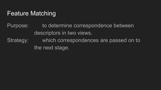
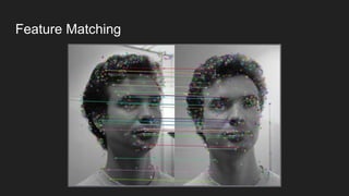
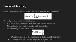
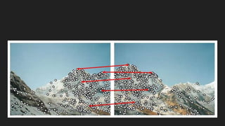
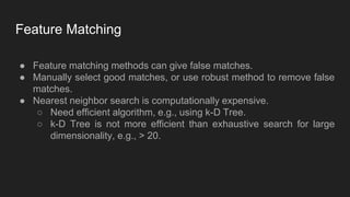
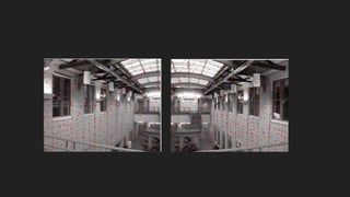
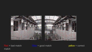
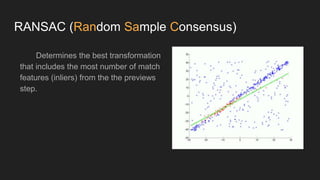
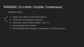
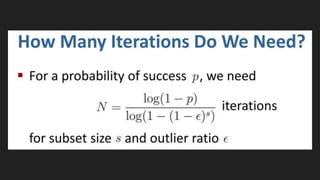
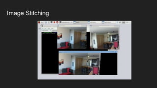
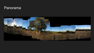
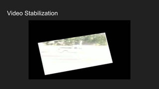
Feature Matching w/
RANSAC
Autor | Calcaben | Obero
Previously on CMSC170
Feature Detection
Previously on CMSC170
Feature Detection
Previously on CMSC170
Feature Detection
Previously on CMSC170
Feature Descriptions
Previously on CMSC170
Feature Descriptions
Feature Matching w/
RANSAC
Autor | Calcaben | Obero
Feature Matching
Purpose: to determine correspondence between
descriptors in two views.
Strategy: which correspondences are passed on to
the next stage.
Feature Matching
Feature Matching
Measure difference as Euclidean distance between feature vectors:
Several possible matching strategies:
● Return all feature vectors with d smaller than a threshold.
● Nearest neighbor: feature vector with smallest d.
● Nearest neighbor distance ratio:
❖ d1, d2: distances to the nearest and 2nd nearest neighbors.
❖ If NNDR is small, nearest neighbor is a good match.
Feature Matching
Feature Matching
● Feature matching methods can give false matches.
● Manually select good matches, or use robust method to remove false
matches.
● Nearest neighbor search is computationally expensive.
○ Need efficient algorithm, e.g., using k-D Tree.
○ k-D Tree is not more efficient than exhaustive search for large
dimensionality, e.g., > 20.
Red = bad match Blue = good match yellow = correct
match
RANSAC (Random Sample Consensus)
Determines the best transformation
that includes the most number of match
features (inliers) from the the previews
step.
RANSAC (Random Sample Consensus)
RANSAC loop:
1. Select four feature pairs (at random)
2. Compute homography H (exact)
3. Compute inliers where SSD(pi’, Hpi) < ε
4. Keep largest set of inliers
5. Re-compute least-squares H estimate on all of the inliers
Homography
a transformation ( a 3×3 matrix ) that maps the points in one image to the
corresponding points in the other image.
Homography
Four corresponding points in
four different colors — red,
green, yellow and orange
Homography
Now since a homography is a 3×3 matrix we can write it as:
Let us consider the first set of corresponding points —(x1,y1) in the first image
and (x2,y2) in the second image. Then, the Homography H maps them in the
following way:
Homography
Pros and Cons
Pros
1. Simple and General
2. Applicable to many different problems
3. Often works well in practice
a. Robust estimation
b. Output acquire relatively high accuracy
Cons
1. Random Nature
2. Lots of Parameters to tune
3. High Computation Time
a. Number of iterations required
4. Can fail for extremely Low Inlier Ratios
a. Extremely sensitive to its threshold value
Applications
Image Stitching
Panorama
Long Screenshot
Screen #1
Screen #2
Screen #3
Screen #4
Screen #5
Screen #6
Video Stabilization
360-degree image
Google Map - Street view
Code Demo
References
https://www.learnopencv.com/homography-examples-using-opencv-python-c/
https://docs.opencv.org/3.4.1/d9/dab/tutorial_homography.html
https://people.cs.umass.edu/~elm/Teaching/ppt/370/370_10_RANSAC.pptx.pdf

Computer Vision: Feature matching with RANSAC Algorithm