Download as PDF, PPTX


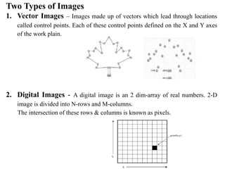

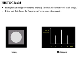
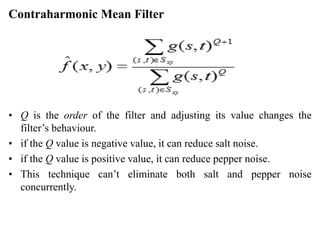
![Inverse filter
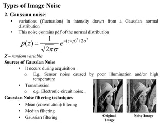
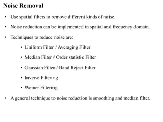
• Compute an estimate F’( u, v) of the transform of the original image by:
• 𝐹′ 𝑢, 𝑣 =
𝐺(𝑢,𝑣)
𝐻(𝑢,𝑣)
• Divisions are made between individual elements of the functions.
• 𝐹′ 𝑢, 𝑣 = 𝐹 𝑢, 𝑣 +
𝑁(𝑢,𝑣)
𝐻(𝑢,𝑣)
• Equation shows that even if we know degradation function, we can not
recover the undegraded image [Inverse Fourier Transform of F(u, v)]
exactly, because N(u, v) is random function whose Fourier Transform is
not known.
• If degradation has ZERO or less value then N(u, v) / H(u, v) dominates
the estimated F’(u, v).
• No explicit provision for handling Noise.](https://image.slidesharecdn.com/imageprocessing-210816071030/85/Image-processing-Noise-Noise-Removal-filters-39-320.jpg)
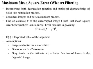
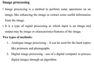
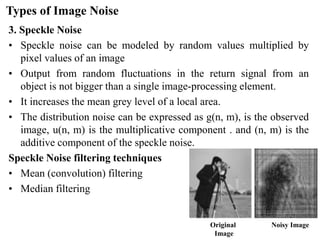
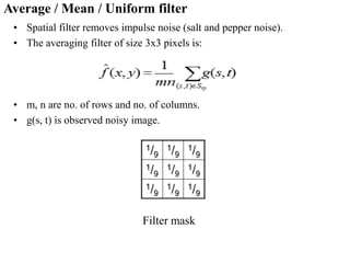
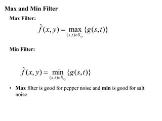
![Maximum Mean Square Error (Wiener) Filtering
Based on these conditions:
• F’(u,v) =[1/H(u,v)] [ |H(u,v|2 / (|H(u,v|2 +S(u,v)/Sf(u,v))] G(u,v)
• H(u,v) – degraded function
• H * (u,v) – complecx conjugate of H(u,v)
• H(u,v) = H * (u,v)H(u,v)
• S(u,v) = |N(u,v)|2 power spectrum of noise
• Sf(u,v) = |F(u,v)|2 power spectrum of undegraded image](https://image.slidesharecdn.com/imageprocessing-210816071030/85/Image-processing-Noise-Noise-Removal-filters-41-320.jpg)

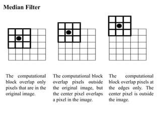
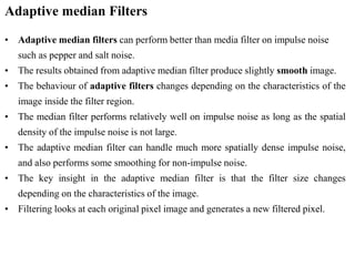
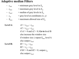
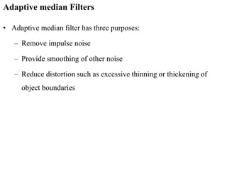
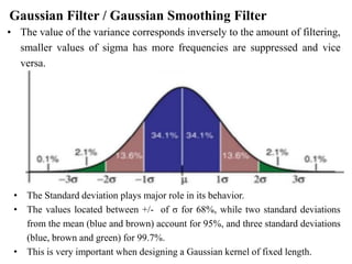
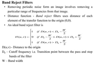
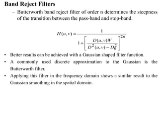
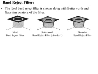
The document covers image processing, defining types of images, image formation, and various noise types encountered in images. It details noise reduction techniques and filtering methods such as mean, median, and Gaussian filters to address different types of noise like salt and pepper, Gaussian, and periodic noise. The document also discusses adaptive filtering methods and their advantages in processing images with varying impulse noise densities.