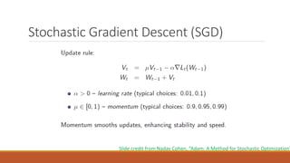
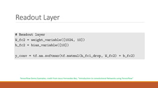
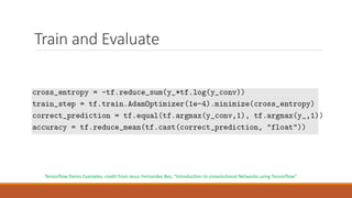
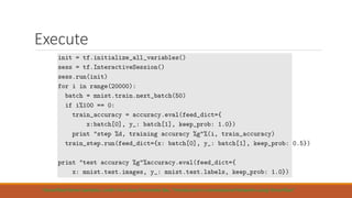
Downloaded 522 times
![What is Convolutional Neural Network?
What is convolution?
◦ It is a specialized linear operation.
◦ A 2D convolution is shown on the right. (Images From: community.arm.com)
◦ Strictly speaking, it’s cross-correlation.
◦ In CNNs, all convolution operations are actually cross-correlation.
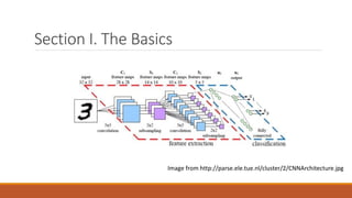
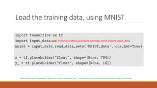
Convolutional neural networks are neural networks that use convolution in place of general
matrix multiplication in at least one of their layers. They are very powerful in processing data
with grid-like topology. [1]
[1] Ian Goodfellow, Yoshua Bengio, Aaron Courville , Deep Learning](https://image.slidesharecdn.com/convolutionalneuralnetworkhengyanglu-170520023530/85/Convolutional-neural-network-4-320.jpg)
![MNIST Classification Record [1]
Classifier Preprocessing Best Test Error Rate (%)
Linear Classifiers deskewing 7.6
K-Nearest Neighbours Shape-context feature extraction 0.63
Boosted Stumps Haar features 0.87
Non-linear classifiers none 3.3
SVMs deskewing 0.56
Neural Nets none 0.35
Convolution Neural Nets Width normalization 0.23
[1] http://yann.lecun.com/exdb/mnist/](https://image.slidesharecdn.com/convolutionalneuralnetworkhengyanglu-170520023530/85/Convolutional-neural-network-9-320.jpg)
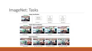
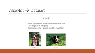
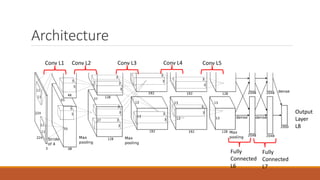
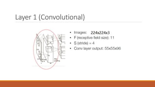
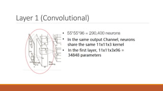
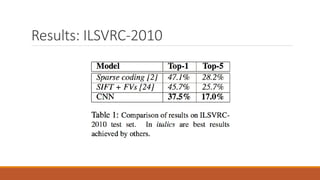
![The ImageNet Challenge [1][2]
The ImageNet Large Scale Visual Recognition Challenge (ILSVRC) is a benchmark in object
category classification and detection on hundreds of object categories and millions of images
◦ The ILSVRC challenge has been running annually since 2010, following the footsteps of PASCAL VOC
challenge, which was established in 2005.
◦ ILSVRC 2010, 1,461406 images and 1000 object classes.
◦ Images are annotated, and annotations fall into one of two categories
◦ (1) image-level annotation of a binary label for the presence or absence of an object class in the image;
◦ (2) object-level annotation of a tight bounding box and class label around an object instance in the image.
◦ ILSVRC 2017, the last ILSVRC challenge.
◦ In these years, several convolutional neural network structure won the first place:
◦ AlexNet 2012
◦ InceptionNet 2014
◦ Deep Residual Network 2015
[1] http://image-net.org/challenges/LSVRC/2017/
[2] Olga Russakovsky et al., ImageNet Large Scale Visual Recognition Challenge](https://image.slidesharecdn.com/convolutionalneuralnetworkhengyanglu-170520023530/85/Convolutional-neural-network-10-320.jpg)

![Technology Behind PRISMA [1]
Deep Convolutional Neural Networks
(a) Separate the content and style of an image
(b) Recombine the content of one image with
the style of another image
[1] Leon A. Gatys et al, A Neural Algorithm of Artistic Style](https://image.slidesharecdn.com/convolutionalneuralnetworkhengyanglu-170520023530/85/Convolutional-neural-network-15-320.jpg)
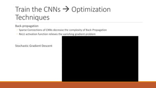
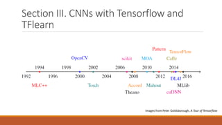
![Section II: More Details [1]
http://www.ritchieng.com/machine-learning/deep-learning/convs/
[1] Slides in section II, credit from slides presented by Tugce Tasci and Kyunghee Kim](https://image.slidesharecdn.com/convolutionalneuralnetworkhengyanglu-170520023530/85/Convolutional-neural-network-17-320.jpg)


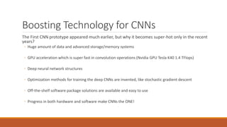
The document presents an overview of Convolutional Neural Networks (CNNs), detailing their advantages over traditional neural networks, specific architectures like AlexNet, and their performance in tasks such as image classification and object detection. It highlights the role of deep learning techniques and technologies that have contributed to the rise of CNNs, including improved optimization methods and powerful computational resources. Additionally, it discusses the use of TensorFlow and TFLearn for implementing CNNs, emphasizing the state-of-the-art results achieved with these models while acknowledging ongoing challenges in interpreting their mechanisms.