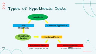
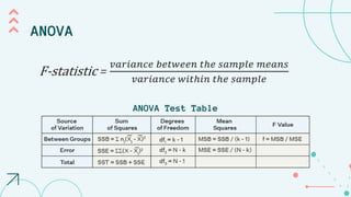
This document provides an overview of parametric and non-parametric hypothesis tests. It defines parametric tests as those that assume an underlying normal distribution, and lists common parametric tests like the z-test, t-test, F-test, and ANOVA. Non-parametric tests make no distributional assumptions and common examples discussed include the Mann-Whitney U test, chi-square test, and Kruskal-Wallis test. The document provides details on assumptions and procedures for conducting each of these important statistical hypothesis tests.

1. Hypothesis
Testing
Aadarsh Agarwal
Kratu Gupta

2. Table of contents
01
02
03
Definition
Non Parametric Tests
Parametric Tests

3. Definition
01

4. Hypothesis Testing
Hypothesis testing is one of the most
important concepts in Statistics which is
heavily used by Statisticians, Machine
Learning Engineers, and Data Scientists.
In hypothesis testing, Statistical tests are
used to check whether the null hypothesis
is rejected or not rejected. These Statistical
tests assume a null hypothesis of no
relationship or no difference between
groups.

5. Types of Hypothesis Tests
Hypothesis
Null
Hypothesis
Alternate Hypothesis
Hypothesis
Testing
Statistical Tests
Non-Parametric
Tests
Parametric Tests
Z-Test, T-test, F-test, ANOVA Chi-Square Test, U-Test, H-Test

6. Parametric Tests
02

7. Definition
Parametric tests are those tests for which we have prior knowledge of the population
distribution (i.e., normal), or if not then we can easily approximate it to a normal
distribution which is possible with the help of the Central Limit Theorem.
Some of the available parametric tests are as follows:
01
02
To find the confidence interval
for the population means with
the help of known standard
deviation.
To determine the confidence
interval for population means
along with the unknown
standard deviation.
04
05
To find the confidence interval
for the population variance.
To find the confidence interval
for the difference of two
means, with an unknown value
of standard deviation.

8. T-Test
03

9. Assumptions
● Population distribution is normal
● Samples are random and independent
● The sample size is small.
● Population standard deviation is not known.

10. One Sample T - test
Types of T-test
Two Sample T – test
where,
x̄ is the sample mean
s is the sample standard deviation
n is the sample size
μ is the population mean
where,
x̄1 is the sample mean of the first group
x̄2 is the sample mean of the second group
S1 is the sample-1 standard deviation
S2 is the sample-2 standard deviation
N1 and N2 are the sample sizes

11. Z - test
04

12. Assumptions
● Population distribution is normal
● Samples are random and independent.
● The sample size is large.
● Population standard deviation is known.

13. One Sample T - test
Types of Z-test
Two Sample T – test
where,
x̄ is the sample mean
σ is the sample standard
deviation
n is the sample size
μ is the population mean
where,
x̄1 is the sample mean of the first group
x̄2 is the sample mean of the second group
σ1 is the sample-1 standard deviation
σ2 is the sample-2 standard deviation
n1 and n2 are the sample sizes

14. F - test
05

15. Assumptions
● Population distribution is normal
● Samples are drawn randomly and independently.

16. Formulation of F-test
F =
s1
2
s2
2
By changing the variance in the ratio, F-test has become a
very flexible test. It can then be used to:
• Test the overall significance for a regression model.
• To compare the fits of different models and
• To test the equality of means.

17. ANOVA
06

18. Assumptions
● Population distribution is normal
● Samples are random and independent
● Homogeneity of sample variance
One-way ANOVA and Two-way ANOVA are its
types

19. ANOVA
F-statistic =
𝑣𝑎𝑟𝑖𝑎𝑛𝑐𝑒 𝑏𝑒𝑡𝑤𝑒𝑒𝑛 𝑡ℎ𝑒 𝑠𝑎𝑚𝑝𝑙𝑒 𝑚𝑒𝑎𝑛𝑠
𝑣𝑎𝑟𝑖𝑎𝑛𝑐𝑒 𝑤𝑖𝑡ℎ𝑖𝑛 𝑡ℎ𝑒 𝑠𝑎𝑚𝑝𝑙𝑒
ANOVA Test Table

20. WHAT IF WE DON’T KNOW
THE DISTRIBUTION?

21. NON-PARAMETRIC TESTS
07

22. Definition
Non-parametric tests are statistical tests that do not make
assumptions about the underlying distribution of the data. These tests
are often used when the data is not normally distributed or when the
sample size is small.
Some of the tests are Spearman Rank Correlation Test, Chi-Square Test,
Mann Whitney U test, Kruskal Wallis Test.

23. MANN-WHITNEY U TEST
08

24. Also known as the Wilcoxon rank-sum test , it is used to
investigate whether two independent samples were selected from a
population having the same distribution.
It is a true non-parametric counterpart of the T-test and gives
the most accurate estimates of significance especially when sample
sizes are small and the population is not normally distributed.

25. Suppose we have two independent groups of data, group A and group B,
and we want to test whether there is a significant difference between
the distributions of the two groups.
Group A: 5, 7, 8, 9, 10 Group B: 2, 4, 6, 8, 12
Step 1: Combine the two groups of data into one ranked list,
assigning ranks to each data point.
Combined ranked list: 1, 2, 3, 4, 5, 6, 7, 8
Corresponding data values: 2, 4, 5, 6, 7, 8, 9, 12
Group A: 5, 7, 8, 9, 10 Ranked: 3, 4, 5, 6, 7
Group B: 2, 4, 6, 8, 12 Ranked: 1, 2, 3, 4, 8

26. Step 2: Calculate the sum of the ranks for each group, denoted as U1 and U2.
U1 = sum of the ranks in group A = 3 + 4 + 5 + 6 + 7 = 25
U2 = sum of the ranks in group B = 1 + 2 + 3 + 4 + 8 = 18
Step 3:
Calculate the test statistic, U, as the smaller of U1 and U2.
U = min(U1, U2) = min(25, 18) = 18

27. Step 4: Calculate the critical value of U using a table or software, based on
the sample size and desired level of significance. For example, at a
significance level of 0.05 with a sample size of 5 in each group, the
critical value of U is 5.
Step 5:
In this example, the test statistic (U = 18) is greater than the critical
value (5), so we fail to reject the null hypothesis and conclude that there
is not enough evidence to suggest that the distributions of the two groups
are different.

28. CHI-SQUARE TEST
09

29. The chi-square test is a statistical test used to determine if there is a
significant association between two categorical variables. It is a
nonparametric test, which means that it does not make any assumptions about
the distribution of the data.
There are two types of chi-square tests: the chi-square goodness-of-fit test
and the chi-square test for independence.

30. The steps for conducting a chi-square test are as follows:
State the null and alternative hypotheses
Calculate the expected frequencies
Calculate the test statistic
χ² = Σ ((O - E)² / E)
Determine the degrees of freedom
Compare the test statistic to the critical value

31. Suppose we want to determine if there is an association between gender and
smoking status. We randomly select 200 individuals and collect data on their
gender and smoking status, resulting in the following contingency table:
Smoker Non-Smoker Total
Male 40 60 100
Female 35 65 100
Total 75 125 200

32. We calculate expected frequencies:
Smoker Non-Smoker Total
Male 35 65 100
Female 35 65 100
Total 70 130 200

33. Now, we will calculate test statistics:
X² = ((40 - 35)² / 35) + ((60 - 65)² / 65) + ((30 - 35)² / 35) + ((70 - 65)²
/ 65) = 2.76
Calculate the Degrees of freedom & Compare it with tabulated value at 0.05
level of significance which is 3.841.
Since the test statistic (2.76) is less than the critical value (3.841), we
fail to reject the null hypothesis and conclude that there is no significant
difference between the observed and expected frequencies.

34. SPEARMAN RANK CORRELATION TEST
10

35. The Spearman rank correlation test is a non-parametric statistical method
used to measure the strength and direction of the association between two
variables. This test is used when the data is ordinal, meaning that it is
ranked in order, but not necessarily evenly spaced.
The test is based on calculating a correlation coefficient, denoted by the
symbol rho (ρ), which ranges from -1 to 1.
Test statistic:
rs = 1 - (6Σd² / n(n²-1))
where rs is the Spearman rank correlation coefficient,
d is the difference in ranks,
and n is the sample size.

36. KRUSKAL-WALLIS TEST
11

37. The Kruskal-Wallis test is a nonparametric test used to compare the
medians of three or more independent groups. It is often used as an
alternative to the one-way analysis of variance (ANOVA) when the
assumption of normality is violated, or when the data is ordinal or
categorical.
H = [(12 / (n(n+1))) * Σ(Rj - (n+1)/2)²] - 3(n+1)
where H is the Kruskal-Wallis test statistic,
n is the total number of observations across all groups,
Rj is the sum of the ranks in group j,
and Σ is the sum of all the groups.

38. Suppose we want to determine if there is a significant difference in the
median salaries of employees across four different departments. The data is
as follows:
Department 1: 35k, 40k, 42k, 45k
Department 2: 30k, 33k, 37k, 38k
Department 3: 43k, 45k, 47k, 50k
Department 4: 32k, 36k, 40k, 42k

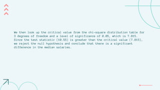
39. We first rank the data:
Rank: 30, 32, 33, 35, 36, 37, 38, 40, 40, 42, 42, 43, 45, 45, 47, 50
H = [(12 / (n(n+1))) * Σ(Rj - (n+1)/2)²] - 3(n+1)
We then calculate the test statistic:
H = [(12 / (16(16+1))) * Σ(Rj - (16+1)/2)²] - 3(16+1)
= [(12 / 272) * ((10.5-8)² + (14.5-8)² + (26.5-8)² + (21.5-8)²)] - 51
= 10.55
Degrees of freedom = number of groups - 1 = 4 - 1 = 3

40. We then look up the critical value from the chi-square distribution table for
3 degrees of freedom and a level of significance of 0.05, which is 7.815.
Since the test statistic (10.55) is greater than the critical value (7.815),
we reject the null hypothesis and conclude that there is a significant
difference in the median salaries.

41. THANK YOU!