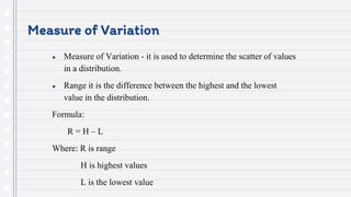
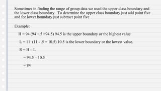
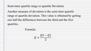
SlideShare a Scribd company logo
Measure of Variation
● Measure of Variation - it is used to determine the scatter of values
in a distribution.
● Range it is the difference between the highest and the lowest
value in the distribution.
Formula:
R = H – L
Where: R is range
H is highest values
L is the lowest value
Steps:
1. Determined the lowest value.
2. Determined the highest value.
3. Substitute the given values in the formula.
4. Solve the problem.
Example:
Statistics classes with 60 students were given an examination and the results are the following:
48 73 57 57 69 88 11 80 82 47
46 70 49 45 75 81 33 65 38 59
94 59 62 36 58 69 45 55 58 65
30 49 73 29 41 53 37 35 61 48
22 51 56 55 60 37 56 59 57 36
12 36 50 63 68 30 56 70 53 28
Solution:
1. Determined the lowest value.
L = 11
2. Determined the highest value.
H = 94
3. Substitute the given values in the formula.
R = H – L
= 94 – 11
4. Solve the problem.
R = H – L
= 94 – 11
= 83
Sometimes in finding the range of group data we used the upper class boundary and
the lower class boundary. To determine the upper class boundary just add point five
and for lower boundary just subtract point five.
Example:
H = 94 (94 +.5 =94.5) 94.5 is the upper boundary or the highest value
L = 11 (11 - .5 = 10.5) 10.5 is the lower boundary or the lowest value.
R = H – L
= 94.5 – 10.5
= 84
Semi-inter quartile range or quartile Deviation
Another measure of deviation is the semi-inter quartile
range or quartile deviation. This value is obtained by getting
one half the differences between the third and the first
quartiles.
Formula:
𝑄 =
𝑄3 − 𝑄1
2
Example:
The examination score of 50 students in a statistics class resulted to the
following values: Q3 = 75. 43 and Q1 = 54.24. Determine the value of the semi-
inter quartile range.
Given:
Q3 = 75. 43
Q1 = 54.24
Q = ?
Solution:
𝑄 =
𝑄3 − 𝑄1
2
𝑄 =
75.43 − 54.24
2
𝑄 =
21.19
2
𝑄 = 10.60
Another Example:
Suppose the performance rating of 100 faculty members of a certain college
were taken and are presented in a frequency distribution as follows:
Classes f
71-74 3
75-78 10
79-82 13
83-86 18
87-90 25
91-94 19
95-98 12
n = 100
Solution:
We will first compute the value of Q3 and Q1 since only the frequency
distribution is given.
Classes f <cumf
71-74 3 3
75-78 10 13
79-82 13 26 (1st Quartile class)
83-86 18 44
87-90 25 69
91-94 19 88 (3rd Quartile class)
95-98 12 100
Formula:
𝑄1 = 𝑥𝑙𝑏 + (
n
4
−𝑐𝑢𝑚𝑓𝑏
𝑓𝑄1
)𝑐
Solution:
𝑄1 = 𝑥𝑙𝑏 + (
n
4
−𝑐𝑢𝑚𝑓𝑏
𝑓𝑄1
)𝑐
𝑄1 = 78.5 + (
25−13
13
)4
𝑄1 = 78.5 + (
12
13
)4
𝑄1 = 78.5 + (0.923076923)4
𝑄1 = 78.5 + 3.692307692
𝑄1 = 82.19230769 or 82.19
Formula:
𝑄3 = 𝑥𝑙𝑏 + (
3n
4
−𝑐𝑢𝑚𝑓𝑏
𝑓𝑄3
)𝑐
Solution:
𝑄3 = 𝑥𝑙𝑏 + (
3n
4
−𝑐𝑢𝑚𝑓𝑏
𝑓𝑄3
)𝑐
𝑄3 = 90.5 + (
75−69
19
)4
𝑄3 = 90.5 + (
6
19
)4
𝑄3 = 90.5 + (0.315789473)4
𝑄3 = 90.5 + 1.263157895
𝑄3 = 91.7631579 𝑜𝑟 91.76
The value of Q can now be obtained. Thus,
𝑄 =
𝑄3−𝑄1
2
𝑄 =
91.76−82.19
2
𝑄 =
9.57
2
𝑄 = 4.78
Average Deviation
● The average deviation refers to the
arithmetic mean of the absolute deviations
of the values from the mean of the
distribution. This measure in sometimes
referred to as the mean absolute deviation.
Average Deviation for Ungroup Data
AD =
|x − 𝒙|
𝒏
where: x represents the individual values
𝒙 is the mean of the distribution
Average Deviation of Ungrouped Data
Steps:
1. Arrange the values in column according to magnitude.
2. Computed the value of the mean (𝒙).
3. Determine the deviations (𝒙 − 𝒙)
4. Convert the deviations in step 3 into positive deviations. Use the absolute
values sign |x− 𝒙|
5. Get the sum of the absolute deviations in step 4.
6. Divide the sum in step 5 by n.
Example:
Consider the following values.
x: 13, 16, 9, 6, 15, 7, 11
Determined the value of the average deviation.
Solution:
First we arrange the values in vertical column and then we compute the
value of the mean.
Step 1: Step 2: Step 3:
x x x − 𝒙
6 𝒙 =
𝒙
𝒏
6 6 – 11 = -5
7 7 7 – 11 = -4
9 =
𝟕𝟕
𝟕
9 9 – 11 = -2
11 11 11 – 11 = 0
13 = 11 13 13 – 11 = 2
15 15 15 – 11 = 4
16 16 16 – 11 = 5
𝒙 = 𝟕𝟕
Step 4:
x x − 𝒙 |x − 𝒙|
6 6 – 11 = -5 5
7 7 – 11 = -4 4
9 9 – 11 = -2 2
11 11 – 11 = 0 0
13 13 – 11 = 2 2
15 15 – 11 = 4 4
16 16 – 11 = 5 5
Notice that the some of the deviations from negative. Hence, we make an
assumption that all deviations are positive deviations by introducing the absolute
value sign. Adding all these absolute deviations.
Step 5: Step 6:
x x − 𝒙 |x − 𝒙| AD =
|x − 𝒙|
𝒏
6 6 – 11 = -5 5
7 7 – 11 = -4 4 =
𝟐𝟐
𝟕
9 9 – 11 = -2 2
11 11 – 11 = 0 0 = 3.14
13 13 – 11 = 2 2
15 15 – 11 = 4 4
16 16 – 11 = 5 5
|x − 𝒙| = 𝟐𝟐
Average Deviation for Group Data
AD =
𝒇|x − 𝒙|
𝒏
Where:
f – represent the frequency of each class
x – the midpoint of each class
𝒙- The mean of the distribution
n – the total number of frequency.
Average Deviation for Group Data
Steps:
1. Compute the value of mean.
2. Get the deviation by using the expression 𝒙 − 𝒙.
3. Multiply the deviation by its corresponding frequency.
4. Add the results in step 3
5. Divide the sum in step 4 by n.
Example:
Compute the value of the average deviation of the frequency distribution as follows:
Classes f
11-22 3
23-34 5
35-46 11
47-58 19
59-70 14
71-82 6
83-94 2
n = 60
Solution:
Step 1: compute the value of the mean
𝑥 =
𝑓𝑥
𝑛
=
3174
60
= 52.90
Classes f x fx
11-22 3 16.5 49.5
23-34 5 28.5 142.5
35-46 11 40.5 445.5
47-58 19 52.5 997.5
59-70 14 64.5 903.0
71-82 6 76.5 459.0
83-94 2 88.5 177.0
n = 60
𝒇𝒙 = 𝟑, 𝟏𝟕𝟒
Step 2: Construct the deviation column 𝒙 − 𝒙
𝒙 − 𝒙
16.5 – 52.90 = -36.4
28.5 – 52.90 = -24.4
40.5 – 52.90 = -12.4
52.5 – 52.90 = -0.4
64.5 – 52.90 = 11.6
76.5 – 52.90 = 23.6
88.5 – 52.90 = 35.6
Classes f x fx 𝒙 − 𝒙
11-22 3 16.5 49.5 -36.4
23-34 5 28.5 142.5 -24.4
35-46 11 40.5 445.5 -12.4
47-58 19 52.5 997.5 -0.4
59-70 14 64.5 903.0 11.6
71-82 6 76.5 459.0 23.6
83-94 2 88.5 177.0 35.6
Step 3: Convert the deviations to positive deviations
Classes f x fx 𝒙 − 𝒙 |x− 𝒙|
11-22 3 16.5 49.5 -36.4 36.4
23-34 5 28.5 142.5 -24.4 24.4
35-46 11 40.5 445.5 -12.4 12.4
47-58 19 52.5 997.5 -0.4 0.4
59-70 14 64.5 903.0 11.6 11.6
71-82 6 76.5 459.0 23.6 23.6
83-94 2 88.5 177.0 35.6 35.6
Step 4: multiply the positive deviations by their corresponding frequencies.
Classes f x fx 𝒙 − 𝒙 |x− 𝒙| f |x− 𝒙|
11-22 3 16.5 49.5 -36.4 36.4 109.2
23-34 5 28.5 142.5 -24.4 24.4 122.0
35-46 11 40.5 445.5 -12.4 12.4 136.4
47-58 19 52.5 997.5 -0.4 0.4 7.6
59-70 14 64.5 903.0 11.6 11.6 162.4
71-82 6 76.5 459.0 23.6 23.6 141.6
83-94 2 88.5 177.0 35.6 35.6 71.2
n = 60 ∑fx = 3,174 ∑f |x− 𝒙| = 750.4
Step 5: Divide the sum in step 4 by n
AD =
𝒇|x − 𝒙|
𝒏
=
750.4
60
= 12.51
Variance
● In the preceding sections, we noticed that the sum of the
deviations from the mean equals 0 if the signs are
considered. If the signs are ignored, that is, assuming
that all the deviations are positive numbers, then the
sum will also be a positive number. In these sections,
we shall consider another procedure of handling signed
numbers. If the deviations 𝑥 − 𝑥 are squared, then the
sum of the squared deviations will also be equal to a
positive number. If this sum is divided by the sample
size n, then we will be able to come up with the mean of
squared deviations. We shall call this measure the
variance.
Variance for Ungrouped Data
𝑺𝟐 =
|x − 𝒙|𝟐
𝒏
where: x represents the individual values in the distribution
𝒙 is the mean of the distribution
n is the sample size
Steps:
1. Computed the value of the mean (𝒙).
2. Get the deviation of each value from mean
3. Square the deviations
4. Calculate the sum of the squared deviations
5. Divide the sum by the total number of values.
Example:
Compute the value of variance of the following measurements
x: 13, 5, 7, 9, 10, 17, 15, 12
Step 1: Compute the Value of Mean
x
5
7
9
10
12
13
15
17
𝒙 = 88
𝒙 =
𝒙
𝒏
= 88/8
= 11
Step 2: Get the deviation of each value from mean
x 𝒙 x − 𝒙
5 11 -6
7 11 -4
9 11 -2
10 11 -1
12 11 1
13 11 2
15 11 4
17 11 6
𝐱 = 88
Step 3: Square the deviations
x x − 𝒙 (x − 𝒙) 2
5 -6 36
7 -4 16
9 -2 4
10 -1 1
12 1 1
13 2 4
15 4 16
17 6 36
𝐱 = 88
Step 4: Calculate the sum of squared deviation
x x − 𝒙 (x − 𝒙) 2
5 -6 36
7 -4 16
9 -2 4
10 -1 1
12 1 1
13 2 4
15 4 16
17 6 36
𝒙 = 88 = 114
Step 5:
𝑺𝟐 =
|x − 𝒙|
𝟐
𝒏
=
𝟏𝟏𝟒
𝟖
= 14.25
Variance for Grouped Data
The computing formulas for the variance as in 𝑠2 =
𝑓 𝑥−𝐱 2
𝑛
is based on
ungrouped data. When the data are presented in a frequency distribution,
however, we shall have another computing formula.
𝒔𝟐 =
𝒇 𝒙−𝒙 𝟐
𝒏
Where: x is midpoint of each class interval
𝒙 is the mean
n is the sample size
Steps:
1. Compute the value of the mean.
2. Determined the deviation x− x
̄ by subtracting the mean
from the midpoint of each class interval.
3. Square the deviations obtained in step 2.
4. Multiply the frequencies by their corresponding squared
deviations.
5. Add the results in step 4.
6. Divide the result in step 5 by the sample size.
Example:
Calculate the variance of the distribution of the following:
Classes f
11-22 3
23-34 5
35-46 11
47-58 19
59-70 14
71-82 6
83-94 2
𝒇 = 𝟔𝟎
Step 1: Compute the value of the mean
Classes f x fx
11-22 3 16.5 49.5
23-34 5 28.5 142.5
35-46 11 40.5 445.5
47-58 19 52.5 997.5
59-70 14 64.5 903
71-82 6 76.5 459
83-94 2 88.5 177
𝒇 = 𝟔𝟎 𝒇𝒙 = 𝟑𝟏𝟕𝟒
𝒙 =
𝒇𝒙
𝒏
=
𝟑𝟏𝟕𝟒
𝟔𝟎
= 52.90
Step 2: Construct the deviation 𝑥 − 𝑥
Classes f x fx 𝒙 − 𝒙
11-22 3 16.5 49.5 -36.4
23-34 5 28.5 142.5 -24.4
35-46 11 40.5 445.5 -12.4
47-58 19 52.5 997.5 -0.4
59-70 14 64.5 903 11.6
71-82 6 76.5 459 23.6
83-94 2 88.5 177 35.6
Step 3: square the deviation
Classes f x fx 𝒙 − 𝒙 |x − 𝒙|2
11-22 3 16.5 49.5 -36.4 1324.96
23-34 5 28.5 142.5 -24.4 595.36
35-46 11 40.5 445.5 -12.4 153.76
47-58 19 52.5 997.5 -0.4 0.16
59-70 14 64.5 903 11.6 134.56
71-82 6 76.5 459 23.6 556.96
83-94 2 88.5 177 35.6 1267.36
Step 4: Multiply the deviations by their corresponding
frequencies
Classes f x fx 𝒙 − 𝒙 |x − 𝒙|2 f|x − 𝒙|2
11-22 3 16.5 49.5 -36.4 1324.96 3974.88
23-34 5 28.5 142.5 -24.4 595.36 2976.8
35-46 11 40.5 445.5 -12.4 153.76 1691.36
47-58 19 52.5 997.5 -0.4 0.16 3.04
59-70 14 64.5 903 11.6 134.56 1883.84
71-82 6 76.5 459 23.6 556.96 3341.76
83-94 2 88.5 177 35.6 1267.36 2535.92
𝒇 = 𝟔𝟎 𝒇𝒙 = 𝟑𝟏𝟕𝟒 𝒇|x−𝒙| =
𝟏𝟔𝟒𝟎𝟕. 𝟔
Step 5: Divide the sum of Step 4 by n
𝒔𝟐
=
𝒇 𝒙−𝒙 𝟐
𝒏
=
𝟏𝟔𝟒𝟎𝟕.𝟔
𝟔𝟎
= 273.46
Chapter-6-Variance.pptx

More Related Content

What's hot

Solution of non-linear equations
Solution of non-linear equationsSolution of non-linear equations
Solution of non-linear equationsZunAib Ali
 
Metric space
Metric spaceMetric space
Metric space
NaliniSPatil
 
Notes - Graphs of Polynomials
Notes - Graphs of PolynomialsNotes - Graphs of Polynomials
Notes - Graphs of PolynomialsLori Rapp
 
Linear functions
Linear functions Linear functions
Linear functions
Rudyed Dela Cruz
 
1551 limits and continuity
1551 limits and continuity1551 limits and continuity
1551 limits and continuity
Dr Fereidoun Dejahang
 
Vector spaces
Vector spacesVector spaces
Vector spaces
Quasar Chunawala
 
Lesson 27: Integration by Substitution (worksheet solutions)
Lesson 27: Integration by Substitution (worksheet solutions)Lesson 27: Integration by Substitution (worksheet solutions)
Lesson 27: Integration by Substitution (worksheet solutions)
Matthew Leingang
 
FM calculus
FM calculusFM calculus
FM calculus
Mike Hoad
 
Addition and subtraction in polynomials
Addition and subtraction in polynomialsAddition and subtraction in polynomials
Addition and subtraction in polynomialssaidyein
 
5.4 long division
5.4 long division5.4 long division
5.4 long divisionleblance
 
systems of linear equations & matrices
systems of linear equations & matricessystems of linear equations & matrices
systems of linear equations & matricesStudent
 
The chain rule
The chain ruleThe chain rule
The chain rule
J M
 
Newton backward interpolation
Newton backward interpolationNewton backward interpolation
Newton backward interpolation
MUHAMMADUMAIR647
 
Math for Bus. and Eco. Chapter 2
Math for Bus. and Eco. Chapter 2Math for Bus. and Eco. Chapter 2
Math for Bus. and Eco. Chapter 2
Mong Mara
 
Math presentation on domain and range
Math presentation on domain and rangeMath presentation on domain and range
Math presentation on domain and range
Touhidul Shawan
 
Funktion suurin ja pienin arvo laskemalla
Funktion suurin ja pienin arvo laskemallaFunktion suurin ja pienin arvo laskemalla
Funktion suurin ja pienin arvo laskemallateemunmatikka
 
Rational functions
Rational functionsRational functions
Rational functions
20kat06tha
 
Lesson 27: Integration by Substitution (slides)
Lesson 27: Integration by Substitution (slides)Lesson 27: Integration by Substitution (slides)
Lesson 27: Integration by Substitution (slides)
Matthew Leingang
 
Lesson 3: Continuity
Lesson 3: ContinuityLesson 3: Continuity
Lesson 3: Continuity
Matthew Leingang
 
L5 infinite limits squeeze theorem
L5 infinite limits squeeze theoremL5 infinite limits squeeze theorem
L5 infinite limits squeeze theorem
James Tagara
 

What's hot (20)

Solution of non-linear equations
Solution of non-linear equationsSolution of non-linear equations
Solution of non-linear equations
 
Metric space
Metric spaceMetric space
Metric space
 
Notes - Graphs of Polynomials
Notes - Graphs of PolynomialsNotes - Graphs of Polynomials
Notes - Graphs of Polynomials
 
Linear functions
Linear functions Linear functions
Linear functions
 
1551 limits and continuity
1551 limits and continuity1551 limits and continuity
1551 limits and continuity
 
Vector spaces
Vector spacesVector spaces
Vector spaces
 
Lesson 27: Integration by Substitution (worksheet solutions)
Lesson 27: Integration by Substitution (worksheet solutions)Lesson 27: Integration by Substitution (worksheet solutions)
Lesson 27: Integration by Substitution (worksheet solutions)
 
FM calculus
FM calculusFM calculus
FM calculus
 
Addition and subtraction in polynomials
Addition and subtraction in polynomialsAddition and subtraction in polynomials
Addition and subtraction in polynomials
 
5.4 long division
5.4 long division5.4 long division
5.4 long division
 
systems of linear equations & matrices
systems of linear equations & matricessystems of linear equations & matrices
systems of linear equations & matrices
 
The chain rule
The chain ruleThe chain rule
The chain rule
 
Newton backward interpolation
Newton backward interpolationNewton backward interpolation
Newton backward interpolation
 
Math for Bus. and Eco. Chapter 2
Math for Bus. and Eco. Chapter 2Math for Bus. and Eco. Chapter 2
Math for Bus. and Eco. Chapter 2
 
Math presentation on domain and range
Math presentation on domain and rangeMath presentation on domain and range
Math presentation on domain and range
 
Funktion suurin ja pienin arvo laskemalla
Funktion suurin ja pienin arvo laskemallaFunktion suurin ja pienin arvo laskemalla
Funktion suurin ja pienin arvo laskemalla
 
Rational functions
Rational functionsRational functions
Rational functions
 
Lesson 27: Integration by Substitution (slides)
Lesson 27: Integration by Substitution (slides)Lesson 27: Integration by Substitution (slides)
Lesson 27: Integration by Substitution (slides)
 
Lesson 3: Continuity
Lesson 3: ContinuityLesson 3: Continuity
Lesson 3: Continuity
 
L5 infinite limits squeeze theorem
L5 infinite limits squeeze theoremL5 infinite limits squeeze theorem
L5 infinite limits squeeze theorem
 

Similar to Chapter-6-Variance.pptx

Analysis and interpretation of Assessment.pptx
Analysis and interpretation of Assessment.pptxAnalysis and interpretation of Assessment.pptx
Analysis and interpretation of Assessment.pptx
AeonneFlux
 
lesson 4 measures of central tendency copy
lesson 4 measures of central tendency   copylesson 4 measures of central tendency   copy
lesson 4 measures of central tendency copy
Nerz Baldres
 
Mean of grouped data
Mean of grouped dataMean of grouped data
Mean of grouped data
Batangas National High School
 
Measure of central tendency
Measure of central tendencyMeasure of central tendency
Measure of central tendency
HajrahMughal
 
Measures of Spread
Measures of SpreadMeasures of Spread
Measures of Spread
Danica Joy Aquino
 
Group 3 measures of central tendency and variation - (mean, median, mode, ra...
Group 3  measures of central tendency and variation - (mean, median, mode, ra...Group 3  measures of central tendency and variation - (mean, median, mode, ra...
Group 3 measures of central tendency and variation - (mean, median, mode, ra...
reymartyvette_0611
 
STATISTICS
STATISTICSSTATISTICS
STATISTICS
shahzadebaujiti
 
Measures of variability grouped data
Measures of variability grouped dataMeasures of variability grouped data
Measures of variability grouped data
Jean Claudette Tolentino
 
Measures of dispersion range qd md
Measures of dispersion range qd mdMeasures of dispersion range qd md
Measures of dispersion range qd md
RekhaChoudhary24
 
Descriptive Statistic in Assessment 1
Descriptive Statistic in Assessment 1Descriptive Statistic in Assessment 1
Descriptive Statistic in Assessment 1
Ase Reth
 
Measure of dispersion by Neeraj Bhandari ( Surkhet.Nepal )
Measure of dispersion by Neeraj Bhandari ( Surkhet.Nepal )Measure of dispersion by Neeraj Bhandari ( Surkhet.Nepal )
Measure of dispersion by Neeraj Bhandari ( Surkhet.Nepal )Neeraj Bhandari
 
Measure of variability
Measure of variabilityMeasure of variability
Measure of variability
Haneza Farcasa
 
Frequency distribution
Frequency distributionFrequency distribution
Frequency distribution
metnashikiom2011-13
 
MEASURES-OF-CENTRAL-TENDENCY-VARIABILITY-TEAM-S-PERSISTENCE.pptx
MEASURES-OF-CENTRAL-TENDENCY-VARIABILITY-TEAM-S-PERSISTENCE.pptxMEASURES-OF-CENTRAL-TENDENCY-VARIABILITY-TEAM-S-PERSISTENCE.pptx
MEASURES-OF-CENTRAL-TENDENCY-VARIABILITY-TEAM-S-PERSISTENCE.pptx
RochAsuncion
 
Measures of central tendency
Measures of central tendencyMeasures of central tendency
Measures of central tendency
Manu Antony
 
Standard deviation
Standard deviationStandard deviation
G7 Math Q4-Week 7- Ungrouped Data of Measures of Variability.pptx
G7 Math Q4-Week 7- Ungrouped Data of Measures of Variability.pptxG7 Math Q4-Week 7- Ungrouped Data of Measures of Variability.pptx
G7 Math Q4-Week 7- Ungrouped Data of Measures of Variability.pptx
ArnoldMillones4
 
An overview of statistics management with excel
An overview of statistics management with excelAn overview of statistics management with excel
An overview of statistics management with excel
KRISHANACHOUDHARY1
 
Median of grouped data
Median of grouped dataMedian of grouped data
Median of grouped data
Batangas National High School
 

Similar to Chapter-6-Variance.pptx (20)

Analysis and interpretation of Assessment.pptx
Analysis and interpretation of Assessment.pptxAnalysis and interpretation of Assessment.pptx
Analysis and interpretation of Assessment.pptx
 
lesson 4 measures of central tendency copy
lesson 4 measures of central tendency   copylesson 4 measures of central tendency   copy
lesson 4 measures of central tendency copy
 
Mean of grouped data
Mean of grouped dataMean of grouped data
Mean of grouped data
 
Measure of central tendency
Measure of central tendencyMeasure of central tendency
Measure of central tendency
 
Measures of Spread
Measures of SpreadMeasures of Spread
Measures of Spread
 
Group 3 measures of central tendency and variation - (mean, median, mode, ra...
Group 3  measures of central tendency and variation - (mean, median, mode, ra...Group 3  measures of central tendency and variation - (mean, median, mode, ra...
Group 3 measures of central tendency and variation - (mean, median, mode, ra...
 
STATISTICS
STATISTICSSTATISTICS
STATISTICS
 
Measures of variability grouped data
Measures of variability grouped dataMeasures of variability grouped data
Measures of variability grouped data
 
Measures of dispersion range qd md
Measures of dispersion range qd mdMeasures of dispersion range qd md
Measures of dispersion range qd md
 
Assessment compiled
Assessment compiledAssessment compiled
Assessment compiled
 
Descriptive Statistic in Assessment 1
Descriptive Statistic in Assessment 1Descriptive Statistic in Assessment 1
Descriptive Statistic in Assessment 1
 
Measure of dispersion by Neeraj Bhandari ( Surkhet.Nepal )
Measure of dispersion by Neeraj Bhandari ( Surkhet.Nepal )Measure of dispersion by Neeraj Bhandari ( Surkhet.Nepal )
Measure of dispersion by Neeraj Bhandari ( Surkhet.Nepal )
 
Measure of variability
Measure of variabilityMeasure of variability
Measure of variability
 
Frequency distribution
Frequency distributionFrequency distribution
Frequency distribution
 
MEASURES-OF-CENTRAL-TENDENCY-VARIABILITY-TEAM-S-PERSISTENCE.pptx
MEASURES-OF-CENTRAL-TENDENCY-VARIABILITY-TEAM-S-PERSISTENCE.pptxMEASURES-OF-CENTRAL-TENDENCY-VARIABILITY-TEAM-S-PERSISTENCE.pptx
MEASURES-OF-CENTRAL-TENDENCY-VARIABILITY-TEAM-S-PERSISTENCE.pptx
 
Measures of central tendency
Measures of central tendencyMeasures of central tendency
Measures of central tendency
 
Standard deviation
Standard deviationStandard deviation
Standard deviation
 
G7 Math Q4-Week 7- Ungrouped Data of Measures of Variability.pptx
G7 Math Q4-Week 7- Ungrouped Data of Measures of Variability.pptxG7 Math Q4-Week 7- Ungrouped Data of Measures of Variability.pptx
G7 Math Q4-Week 7- Ungrouped Data of Measures of Variability.pptx
 
An overview of statistics management with excel
An overview of statistics management with excelAn overview of statistics management with excel
An overview of statistics management with excel
 
Median of grouped data
Median of grouped dataMedian of grouped data
Median of grouped data
 

More from RiyanElaine

my presentation about Expanded-Definitions.pptx
my presentation about Expanded-Definitions.pptxmy presentation about Expanded-Definitions.pptx
my presentation about Expanded-Definitions.pptx
RiyanElaine
 
my presentation about Space-And-Galaxies.pptx
my presentation about Space-And-Galaxies.pptxmy presentation about Space-And-Galaxies.pptx
my presentation about Space-And-Galaxies.pptx
RiyanElaine
 
computerhardware-160717095805.pptx
computerhardware-160717095805.pptxcomputerhardware-160717095805.pptx
computerhardware-160717095805.pptx
RiyanElaine
 
activity 5.pptx
activity 5.pptxactivity 5.pptx
activity 5.pptx
RiyanElaine
 
GROUP-3-CWTS2.pptx
GROUP-3-CWTS2.pptxGROUP-3-CWTS2.pptx
GROUP-3-CWTS2.pptx
RiyanElaine
 
LESSON-1-Communication-Process.pptx
LESSON-1-Communication-Process.pptxLESSON-1-Communication-Process.pptx
LESSON-1-Communication-Process.pptx
RiyanElaine
 
Presentation 7 (2) (1).pptx
Presentation 7 (2) (1).pptxPresentation 7 (2) (1).pptx
Presentation 7 (2) (1).pptx
RiyanElaine
 
energysystems-150315210756-conversion-gate01 (2).pptx
energysystems-150315210756-conversion-gate01 (2).pptxenergysystems-150315210756-conversion-gate01 (2).pptx
energysystems-150315210756-conversion-gate01 (2).pptx
RiyanElaine
 
FINALS-READINGS.pptx
FINALS-READINGS.pptxFINALS-READINGS.pptx
FINALS-READINGS.pptx
RiyanElaine
 
Leadership-ppt.ppt
Leadership-ppt.pptLeadership-ppt.ppt
Leadership-ppt.ppt
RiyanElaine
 

More from RiyanElaine (10)

my presentation about Expanded-Definitions.pptx
my presentation about Expanded-Definitions.pptxmy presentation about Expanded-Definitions.pptx
my presentation about Expanded-Definitions.pptx
 
my presentation about Space-And-Galaxies.pptx
my presentation about Space-And-Galaxies.pptxmy presentation about Space-And-Galaxies.pptx
my presentation about Space-And-Galaxies.pptx
 
computerhardware-160717095805.pptx
computerhardware-160717095805.pptxcomputerhardware-160717095805.pptx
computerhardware-160717095805.pptx
 
activity 5.pptx
activity 5.pptxactivity 5.pptx
activity 5.pptx
 
GROUP-3-CWTS2.pptx
GROUP-3-CWTS2.pptxGROUP-3-CWTS2.pptx
GROUP-3-CWTS2.pptx
 
LESSON-1-Communication-Process.pptx
LESSON-1-Communication-Process.pptxLESSON-1-Communication-Process.pptx
LESSON-1-Communication-Process.pptx
 
Presentation 7 (2) (1).pptx
Presentation 7 (2) (1).pptxPresentation 7 (2) (1).pptx
Presentation 7 (2) (1).pptx
 
energysystems-150315210756-conversion-gate01 (2).pptx
energysystems-150315210756-conversion-gate01 (2).pptxenergysystems-150315210756-conversion-gate01 (2).pptx
energysystems-150315210756-conversion-gate01 (2).pptx
 
FINALS-READINGS.pptx
FINALS-READINGS.pptxFINALS-READINGS.pptx
FINALS-READINGS.pptx
 
Leadership-ppt.ppt
Leadership-ppt.pptLeadership-ppt.ppt
Leadership-ppt.ppt
 

Recently uploaded

Model Attribute Check Company Auto Property
Model Attribute  Check Company Auto PropertyModel Attribute  Check Company Auto Property
Model Attribute Check Company Auto Property
Celine George
 
2024.06.01 Introducing a competency framework for languag learning materials ...
2024.06.01 Introducing a competency framework for languag learning materials ...2024.06.01 Introducing a competency framework for languag learning materials ...
2024.06.01 Introducing a competency framework for languag learning materials ...
Sandy Millin
 
"Protectable subject matters, Protection in biotechnology, Protection of othe...
"Protectable subject matters, Protection in biotechnology, Protection of othe..."Protectable subject matters, Protection in biotechnology, Protection of othe...
"Protectable subject matters, Protection in biotechnology, Protection of othe...
SACHIN R KONDAGURI
 
Francesca Gottschalk - How can education support child empowerment.pptx
Francesca Gottschalk - How can education support child empowerment.pptxFrancesca Gottschalk - How can education support child empowerment.pptx
Francesca Gottschalk - How can education support child empowerment.pptx
EduSkills OECD
 
CACJapan - GROUP Presentation 1- Wk 4.pdf
CACJapan - GROUP Presentation 1- Wk 4.pdfCACJapan - GROUP Presentation 1- Wk 4.pdf
CACJapan - GROUP Presentation 1- Wk 4.pdf
camakaiclarkmusic
 
Unit 2- Research Aptitude (UGC NET Paper I).pdf
Unit 2- Research Aptitude (UGC NET Paper I).pdfUnit 2- Research Aptitude (UGC NET Paper I).pdf
Unit 2- Research Aptitude (UGC NET Paper I).pdf
Thiyagu K
 
How libraries can support authors with open access requirements for UKRI fund...
How libraries can support authors with open access requirements for UKRI fund...How libraries can support authors with open access requirements for UKRI fund...
How libraries can support authors with open access requirements for UKRI fund...
Jisc
 
Best Digital Marketing Institute In NOIDA
Best Digital Marketing Institute In NOIDABest Digital Marketing Institute In NOIDA
Best Digital Marketing Institute In NOIDA
deeptiverma2406
 
Embracing GenAI - A Strategic Imperative
Embracing GenAI - A Strategic ImperativeEmbracing GenAI - A Strategic Imperative
Embracing GenAI - A Strategic Imperative
Peter Windle
 
A Survey of Techniques for Maximizing LLM Performance.pptx
A Survey of Techniques for Maximizing LLM Performance.pptxA Survey of Techniques for Maximizing LLM Performance.pptx
A Survey of Techniques for Maximizing LLM Performance.pptx
thanhdowork
 
MASS MEDIA STUDIES-835-CLASS XI Resource Material.pdf
MASS MEDIA STUDIES-835-CLASS XI Resource Material.pdfMASS MEDIA STUDIES-835-CLASS XI Resource Material.pdf
MASS MEDIA STUDIES-835-CLASS XI Resource Material.pdf
goswamiyash170123
 
Biological Screening of Herbal Drugs in detailed.
Biological Screening of Herbal Drugs in detailed.Biological Screening of Herbal Drugs in detailed.
Biological Screening of Herbal Drugs in detailed.
Ashokrao Mane college of Pharmacy Peth-Vadgaon
 
The Accursed House by Émile Gaboriau.pptx
The Accursed House by Émile Gaboriau.pptxThe Accursed House by Émile Gaboriau.pptx
The Accursed House by Émile Gaboriau.pptx
DhatriParmar
 
The French Revolution Class 9 Study Material pdf free download
The French Revolution Class 9 Study Material pdf free downloadThe French Revolution Class 9 Study Material pdf free download
The French Revolution Class 9 Study Material pdf free download
Vivekanand Anglo Vedic Academy
 
Language Across the Curriculm LAC B.Ed.
Language Across the  Curriculm LAC B.Ed.Language Across the  Curriculm LAC B.Ed.
Language Across the Curriculm LAC B.Ed.
Atul Kumar Singh
 
Unit 8 - Information and Communication Technology (Paper I).pdf
Unit 8 - Information and Communication Technology (Paper I).pdfUnit 8 - Information and Communication Technology (Paper I).pdf
Unit 8 - Information and Communication Technology (Paper I).pdf
Thiyagu K
 
Multithreading_in_C++ - std::thread, race condition
Multithreading_in_C++ - std::thread, race conditionMultithreading_in_C++ - std::thread, race condition
Multithreading_in_C++ - std::thread, race condition
Mohammed Sikander
 
Chapter -12, Antibiotics (One Page Notes).pdf
Chapter -12, Antibiotics (One Page Notes).pdfChapter -12, Antibiotics (One Page Notes).pdf
Chapter -12, Antibiotics (One Page Notes).pdf
Kartik Tiwari
 
Advantages and Disadvantages of CMS from an SEO Perspective
Advantages and Disadvantages of CMS from an SEO PerspectiveAdvantages and Disadvantages of CMS from an SEO Perspective
Advantages and Disadvantages of CMS from an SEO Perspective
Krisztián Száraz
 
June 3, 2024 Anti-Semitism Letter Sent to MIT President Kornbluth and MIT Cor...
June 3, 2024 Anti-Semitism Letter Sent to MIT President Kornbluth and MIT Cor...June 3, 2024 Anti-Semitism Letter Sent to MIT President Kornbluth and MIT Cor...
June 3, 2024 Anti-Semitism Letter Sent to MIT President Kornbluth and MIT Cor...
Levi Shapiro
 

Recently uploaded (20)

Model Attribute Check Company Auto Property
Model Attribute  Check Company Auto PropertyModel Attribute  Check Company Auto Property
Model Attribute Check Company Auto Property
 
2024.06.01 Introducing a competency framework for languag learning materials ...
2024.06.01 Introducing a competency framework for languag learning materials ...2024.06.01 Introducing a competency framework for languag learning materials ...
2024.06.01 Introducing a competency framework for languag learning materials ...
 
"Protectable subject matters, Protection in biotechnology, Protection of othe...
"Protectable subject matters, Protection in biotechnology, Protection of othe..."Protectable subject matters, Protection in biotechnology, Protection of othe...
"Protectable subject matters, Protection in biotechnology, Protection of othe...
 
Francesca Gottschalk - How can education support child empowerment.pptx
Francesca Gottschalk - How can education support child empowerment.pptxFrancesca Gottschalk - How can education support child empowerment.pptx
Francesca Gottschalk - How can education support child empowerment.pptx
 
CACJapan - GROUP Presentation 1- Wk 4.pdf
CACJapan - GROUP Presentation 1- Wk 4.pdfCACJapan - GROUP Presentation 1- Wk 4.pdf
CACJapan - GROUP Presentation 1- Wk 4.pdf
 
Unit 2- Research Aptitude (UGC NET Paper I).pdf
Unit 2- Research Aptitude (UGC NET Paper I).pdfUnit 2- Research Aptitude (UGC NET Paper I).pdf
Unit 2- Research Aptitude (UGC NET Paper I).pdf
 
How libraries can support authors with open access requirements for UKRI fund...
How libraries can support authors with open access requirements for UKRI fund...How libraries can support authors with open access requirements for UKRI fund...
How libraries can support authors with open access requirements for UKRI fund...
 
Best Digital Marketing Institute In NOIDA
Best Digital Marketing Institute In NOIDABest Digital Marketing Institute In NOIDA
Best Digital Marketing Institute In NOIDA
 
Embracing GenAI - A Strategic Imperative
Embracing GenAI - A Strategic ImperativeEmbracing GenAI - A Strategic Imperative
Embracing GenAI - A Strategic Imperative
 
A Survey of Techniques for Maximizing LLM Performance.pptx
A Survey of Techniques for Maximizing LLM Performance.pptxA Survey of Techniques for Maximizing LLM Performance.pptx
A Survey of Techniques for Maximizing LLM Performance.pptx
 
MASS MEDIA STUDIES-835-CLASS XI Resource Material.pdf
MASS MEDIA STUDIES-835-CLASS XI Resource Material.pdfMASS MEDIA STUDIES-835-CLASS XI Resource Material.pdf
MASS MEDIA STUDIES-835-CLASS XI Resource Material.pdf
 
Biological Screening of Herbal Drugs in detailed.
Biological Screening of Herbal Drugs in detailed.Biological Screening of Herbal Drugs in detailed.
Biological Screening of Herbal Drugs in detailed.
 
The Accursed House by Émile Gaboriau.pptx
The Accursed House by Émile Gaboriau.pptxThe Accursed House by Émile Gaboriau.pptx
The Accursed House by Émile Gaboriau.pptx
 
The French Revolution Class 9 Study Material pdf free download
The French Revolution Class 9 Study Material pdf free downloadThe French Revolution Class 9 Study Material pdf free download
The French Revolution Class 9 Study Material pdf free download
 
Language Across the Curriculm LAC B.Ed.
Language Across the  Curriculm LAC B.Ed.Language Across the  Curriculm LAC B.Ed.
Language Across the Curriculm LAC B.Ed.
 
Unit 8 - Information and Communication Technology (Paper I).pdf
Unit 8 - Information and Communication Technology (Paper I).pdfUnit 8 - Information and Communication Technology (Paper I).pdf
Unit 8 - Information and Communication Technology (Paper I).pdf
 
Multithreading_in_C++ - std::thread, race condition
Multithreading_in_C++ - std::thread, race conditionMultithreading_in_C++ - std::thread, race condition
Multithreading_in_C++ - std::thread, race condition
 
Chapter -12, Antibiotics (One Page Notes).pdf
Chapter -12, Antibiotics (One Page Notes).pdfChapter -12, Antibiotics (One Page Notes).pdf
Chapter -12, Antibiotics (One Page Notes).pdf
 
Advantages and Disadvantages of CMS from an SEO Perspective
Advantages and Disadvantages of CMS from an SEO PerspectiveAdvantages and Disadvantages of CMS from an SEO Perspective
Advantages and Disadvantages of CMS from an SEO Perspective
 
June 3, 2024 Anti-Semitism Letter Sent to MIT President Kornbluth and MIT Cor...
June 3, 2024 Anti-Semitism Letter Sent to MIT President Kornbluth and MIT Cor...June 3, 2024 Anti-Semitism Letter Sent to MIT President Kornbluth and MIT Cor...
June 3, 2024 Anti-Semitism Letter Sent to MIT President Kornbluth and MIT Cor...
 

Chapter-6-Variance.pptx

  • 1. Measure of Variation ● Measure of Variation - it is used to determine the scatter of values in a distribution. ● Range it is the difference between the highest and the lowest value in the distribution. Formula: R = H – L Where: R is range H is highest values L is the lowest value
  • 2. Steps: 1. Determined the lowest value. 2. Determined the highest value. 3. Substitute the given values in the formula. 4. Solve the problem.
  • 3. Example: Statistics classes with 60 students were given an examination and the results are the following: 48 73 57 57 69 88 11 80 82 47 46 70 49 45 75 81 33 65 38 59 94 59 62 36 58 69 45 55 58 65 30 49 73 29 41 53 37 35 61 48 22 51 56 55 60 37 56 59 57 36 12 36 50 63 68 30 56 70 53 28
  • 4. Solution: 1. Determined the lowest value. L = 11 2. Determined the highest value. H = 94 3. Substitute the given values in the formula. R = H – L = 94 – 11 4. Solve the problem. R = H – L = 94 – 11 = 83
  • 5. Sometimes in finding the range of group data we used the upper class boundary and the lower class boundary. To determine the upper class boundary just add point five and for lower boundary just subtract point five. Example: H = 94 (94 +.5 =94.5) 94.5 is the upper boundary or the highest value L = 11 (11 - .5 = 10.5) 10.5 is the lower boundary or the lowest value. R = H – L = 94.5 – 10.5 = 84
  • 6. Semi-inter quartile range or quartile Deviation Another measure of deviation is the semi-inter quartile range or quartile deviation. This value is obtained by getting one half the differences between the third and the first quartiles. Formula: 𝑄 = 𝑄3 − 𝑄1 2
  • 7. Example: The examination score of 50 students in a statistics class resulted to the following values: Q3 = 75. 43 and Q1 = 54.24. Determine the value of the semi- inter quartile range. Given: Q3 = 75. 43 Q1 = 54.24 Q = ?
  • 8. Solution: 𝑄 = 𝑄3 − 𝑄1 2 𝑄 = 75.43 − 54.24 2 𝑄 = 21.19 2 𝑄 = 10.60
  • 9. Another Example: Suppose the performance rating of 100 faculty members of a certain college were taken and are presented in a frequency distribution as follows: Classes f 71-74 3 75-78 10 79-82 13 83-86 18 87-90 25 91-94 19 95-98 12 n = 100
  • 10. Solution: We will first compute the value of Q3 and Q1 since only the frequency distribution is given. Classes f <cumf 71-74 3 3 75-78 10 13 79-82 13 26 (1st Quartile class) 83-86 18 44 87-90 25 69 91-94 19 88 (3rd Quartile class) 95-98 12 100
  • 11. Formula: 𝑄1 = 𝑥𝑙𝑏 + ( n 4 −𝑐𝑢𝑚𝑓𝑏 𝑓𝑄1 )𝑐 Solution: 𝑄1 = 𝑥𝑙𝑏 + ( n 4 −𝑐𝑢𝑚𝑓𝑏 𝑓𝑄1 )𝑐 𝑄1 = 78.5 + ( 25−13 13 )4 𝑄1 = 78.5 + ( 12 13 )4 𝑄1 = 78.5 + (0.923076923)4 𝑄1 = 78.5 + 3.692307692 𝑄1 = 82.19230769 or 82.19 Formula: 𝑄3 = 𝑥𝑙𝑏 + ( 3n 4 −𝑐𝑢𝑚𝑓𝑏 𝑓𝑄3 )𝑐 Solution: 𝑄3 = 𝑥𝑙𝑏 + ( 3n 4 −𝑐𝑢𝑚𝑓𝑏 𝑓𝑄3 )𝑐 𝑄3 = 90.5 + ( 75−69 19 )4 𝑄3 = 90.5 + ( 6 19 )4 𝑄3 = 90.5 + (0.315789473)4 𝑄3 = 90.5 + 1.263157895 𝑄3 = 91.7631579 𝑜𝑟 91.76
  • 12. The value of Q can now be obtained. Thus, 𝑄 = 𝑄3−𝑄1 2 𝑄 = 91.76−82.19 2 𝑄 = 9.57 2 𝑄 = 4.78
  • 13. Average Deviation ● The average deviation refers to the arithmetic mean of the absolute deviations of the values from the mean of the distribution. This measure in sometimes referred to as the mean absolute deviation.
  • 14. Average Deviation for Ungroup Data AD = |x − 𝒙| 𝒏 where: x represents the individual values 𝒙 is the mean of the distribution
  • 15. Average Deviation of Ungrouped Data Steps: 1. Arrange the values in column according to magnitude. 2. Computed the value of the mean (𝒙). 3. Determine the deviations (𝒙 − 𝒙) 4. Convert the deviations in step 3 into positive deviations. Use the absolute values sign |x− 𝒙| 5. Get the sum of the absolute deviations in step 4. 6. Divide the sum in step 5 by n.
  • 16. Example: Consider the following values. x: 13, 16, 9, 6, 15, 7, 11 Determined the value of the average deviation. Solution: First we arrange the values in vertical column and then we compute the value of the mean.
  • 17. Step 1: Step 2: Step 3: x x x − 𝒙 6 𝒙 = 𝒙 𝒏 6 6 – 11 = -5 7 7 7 – 11 = -4 9 = 𝟕𝟕 𝟕 9 9 – 11 = -2 11 11 11 – 11 = 0 13 = 11 13 13 – 11 = 2 15 15 15 – 11 = 4 16 16 16 – 11 = 5 𝒙 = 𝟕𝟕
  • 18. Step 4: x x − 𝒙 |x − 𝒙| 6 6 – 11 = -5 5 7 7 – 11 = -4 4 9 9 – 11 = -2 2 11 11 – 11 = 0 0 13 13 – 11 = 2 2 15 15 – 11 = 4 4 16 16 – 11 = 5 5 Notice that the some of the deviations from negative. Hence, we make an assumption that all deviations are positive deviations by introducing the absolute value sign. Adding all these absolute deviations.
  • 19. Step 5: Step 6: x x − 𝒙 |x − 𝒙| AD = |x − 𝒙| 𝒏 6 6 – 11 = -5 5 7 7 – 11 = -4 4 = 𝟐𝟐 𝟕 9 9 – 11 = -2 2 11 11 – 11 = 0 0 = 3.14 13 13 – 11 = 2 2 15 15 – 11 = 4 4 16 16 – 11 = 5 5 |x − 𝒙| = 𝟐𝟐
  • 20. Average Deviation for Group Data AD = 𝒇|x − 𝒙| 𝒏 Where: f – represent the frequency of each class x – the midpoint of each class 𝒙- The mean of the distribution n – the total number of frequency.
  • 21. Average Deviation for Group Data Steps: 1. Compute the value of mean. 2. Get the deviation by using the expression 𝒙 − 𝒙. 3. Multiply the deviation by its corresponding frequency. 4. Add the results in step 3 5. Divide the sum in step 4 by n.
  • 22. Example: Compute the value of the average deviation of the frequency distribution as follows: Classes f 11-22 3 23-34 5 35-46 11 47-58 19 59-70 14 71-82 6 83-94 2 n = 60
  • 23. Solution: Step 1: compute the value of the mean 𝑥 = 𝑓𝑥 𝑛 = 3174 60 = 52.90 Classes f x fx 11-22 3 16.5 49.5 23-34 5 28.5 142.5 35-46 11 40.5 445.5 47-58 19 52.5 997.5 59-70 14 64.5 903.0 71-82 6 76.5 459.0 83-94 2 88.5 177.0 n = 60 𝒇𝒙 = 𝟑, 𝟏𝟕𝟒
  • 24. Step 2: Construct the deviation column 𝒙 − 𝒙 𝒙 − 𝒙 16.5 – 52.90 = -36.4 28.5 – 52.90 = -24.4 40.5 – 52.90 = -12.4 52.5 – 52.90 = -0.4 64.5 – 52.90 = 11.6 76.5 – 52.90 = 23.6 88.5 – 52.90 = 35.6 Classes f x fx 𝒙 − 𝒙 11-22 3 16.5 49.5 -36.4 23-34 5 28.5 142.5 -24.4 35-46 11 40.5 445.5 -12.4 47-58 19 52.5 997.5 -0.4 59-70 14 64.5 903.0 11.6 71-82 6 76.5 459.0 23.6 83-94 2 88.5 177.0 35.6
  • 25. Step 3: Convert the deviations to positive deviations Classes f x fx 𝒙 − 𝒙 |x− 𝒙| 11-22 3 16.5 49.5 -36.4 36.4 23-34 5 28.5 142.5 -24.4 24.4 35-46 11 40.5 445.5 -12.4 12.4 47-58 19 52.5 997.5 -0.4 0.4 59-70 14 64.5 903.0 11.6 11.6 71-82 6 76.5 459.0 23.6 23.6 83-94 2 88.5 177.0 35.6 35.6
  • 26. Step 4: multiply the positive deviations by their corresponding frequencies. Classes f x fx 𝒙 − 𝒙 |x− 𝒙| f |x− 𝒙| 11-22 3 16.5 49.5 -36.4 36.4 109.2 23-34 5 28.5 142.5 -24.4 24.4 122.0 35-46 11 40.5 445.5 -12.4 12.4 136.4 47-58 19 52.5 997.5 -0.4 0.4 7.6 59-70 14 64.5 903.0 11.6 11.6 162.4 71-82 6 76.5 459.0 23.6 23.6 141.6 83-94 2 88.5 177.0 35.6 35.6 71.2 n = 60 ∑fx = 3,174 ∑f |x− 𝒙| = 750.4
  • 27. Step 5: Divide the sum in step 4 by n AD = 𝒇|x − 𝒙| 𝒏 = 750.4 60 = 12.51
  • 28. Variance ● In the preceding sections, we noticed that the sum of the deviations from the mean equals 0 if the signs are considered. If the signs are ignored, that is, assuming that all the deviations are positive numbers, then the sum will also be a positive number. In these sections, we shall consider another procedure of handling signed numbers. If the deviations 𝑥 − 𝑥 are squared, then the sum of the squared deviations will also be equal to a positive number. If this sum is divided by the sample size n, then we will be able to come up with the mean of squared deviations. We shall call this measure the variance.
  • 29. Variance for Ungrouped Data 𝑺𝟐 = |x − 𝒙|𝟐 𝒏 where: x represents the individual values in the distribution 𝒙 is the mean of the distribution n is the sample size
  • 30. Steps: 1. Computed the value of the mean (𝒙). 2. Get the deviation of each value from mean 3. Square the deviations 4. Calculate the sum of the squared deviations 5. Divide the sum by the total number of values. Example: Compute the value of variance of the following measurements x: 13, 5, 7, 9, 10, 17, 15, 12
  • 31. Step 1: Compute the Value of Mean x 5 7 9 10 12 13 15 17 𝒙 = 88 𝒙 = 𝒙 𝒏 = 88/8 = 11
  • 32. Step 2: Get the deviation of each value from mean x 𝒙 x − 𝒙 5 11 -6 7 11 -4 9 11 -2 10 11 -1 12 11 1 13 11 2 15 11 4 17 11 6 𝐱 = 88
  • 33. Step 3: Square the deviations x x − 𝒙 (x − 𝒙) 2 5 -6 36 7 -4 16 9 -2 4 10 -1 1 12 1 1 13 2 4 15 4 16 17 6 36 𝐱 = 88
  • 34. Step 4: Calculate the sum of squared deviation x x − 𝒙 (x − 𝒙) 2 5 -6 36 7 -4 16 9 -2 4 10 -1 1 12 1 1 13 2 4 15 4 16 17 6 36 𝒙 = 88 = 114
  • 35. Step 5: 𝑺𝟐 = |x − 𝒙| 𝟐 𝒏 = 𝟏𝟏𝟒 𝟖 = 14.25
  • 36. Variance for Grouped Data The computing formulas for the variance as in 𝑠2 = 𝑓 𝑥−𝐱 2 𝑛 is based on ungrouped data. When the data are presented in a frequency distribution, however, we shall have another computing formula. 𝒔𝟐 = 𝒇 𝒙−𝒙 𝟐 𝒏 Where: x is midpoint of each class interval 𝒙 is the mean n is the sample size
  • 37. Steps: 1. Compute the value of the mean. 2. Determined the deviation x− x ̄ by subtracting the mean from the midpoint of each class interval. 3. Square the deviations obtained in step 2. 4. Multiply the frequencies by their corresponding squared deviations. 5. Add the results in step 4. 6. Divide the result in step 5 by the sample size.
  • 38. Example: Calculate the variance of the distribution of the following: Classes f 11-22 3 23-34 5 35-46 11 47-58 19 59-70 14 71-82 6 83-94 2 𝒇 = 𝟔𝟎
  • 39. Step 1: Compute the value of the mean Classes f x fx 11-22 3 16.5 49.5 23-34 5 28.5 142.5 35-46 11 40.5 445.5 47-58 19 52.5 997.5 59-70 14 64.5 903 71-82 6 76.5 459 83-94 2 88.5 177 𝒇 = 𝟔𝟎 𝒇𝒙 = 𝟑𝟏𝟕𝟒 𝒙 = 𝒇𝒙 𝒏 = 𝟑𝟏𝟕𝟒 𝟔𝟎 = 52.90
  • 40. Step 2: Construct the deviation 𝑥 − 𝑥 Classes f x fx 𝒙 − 𝒙 11-22 3 16.5 49.5 -36.4 23-34 5 28.5 142.5 -24.4 35-46 11 40.5 445.5 -12.4 47-58 19 52.5 997.5 -0.4 59-70 14 64.5 903 11.6 71-82 6 76.5 459 23.6 83-94 2 88.5 177 35.6
  • 41. Step 3: square the deviation Classes f x fx 𝒙 − 𝒙 |x − 𝒙|2 11-22 3 16.5 49.5 -36.4 1324.96 23-34 5 28.5 142.5 -24.4 595.36 35-46 11 40.5 445.5 -12.4 153.76 47-58 19 52.5 997.5 -0.4 0.16 59-70 14 64.5 903 11.6 134.56 71-82 6 76.5 459 23.6 556.96 83-94 2 88.5 177 35.6 1267.36
  • 42. Step 4: Multiply the deviations by their corresponding frequencies Classes f x fx 𝒙 − 𝒙 |x − 𝒙|2 f|x − 𝒙|2 11-22 3 16.5 49.5 -36.4 1324.96 3974.88 23-34 5 28.5 142.5 -24.4 595.36 2976.8 35-46 11 40.5 445.5 -12.4 153.76 1691.36 47-58 19 52.5 997.5 -0.4 0.16 3.04 59-70 14 64.5 903 11.6 134.56 1883.84 71-82 6 76.5 459 23.6 556.96 3341.76 83-94 2 88.5 177 35.6 1267.36 2535.92 𝒇 = 𝟔𝟎 𝒇𝒙 = 𝟑𝟏𝟕𝟒 𝒇|x−𝒙| = 𝟏𝟔𝟒𝟎𝟕. 𝟔
  • 43. Step 5: Divide the sum of Step 4 by n 𝒔𝟐 = 𝒇 𝒙−𝒙 𝟐 𝒏 = 𝟏𝟔𝟒𝟎𝟕.𝟔 𝟔𝟎 = 273.46