Analysis of
variance
ONE WAY ANOVA
 IT USED TO ESTIMATE AND COMPARE THE
EFFECTES OF THE Difference treatments on the
response variables
 We do this by estimating and comparing the
treatments means
 When we compare more than two groups based
on one factors.
E.g. If one the car oil company would to like to
compare the effects of three oil type assume that
A,B and C on oil mileage by midsize cars. And the
company select randomly 5 cars from 1000 cars.
There is only one Factor : oil type
Assumptions on one way
ANOVA
1. Constant variance: the populations of values
of the response variable associated with the
treatments have equal variables.
2. Normality: the pupations of the values of the
response variable associated with the
treatments all have normal distributions
3. Independence: the samples of experimental
units associated with the treatments are
randomly selected, independent sample
Testing the significant differences
between treatments means
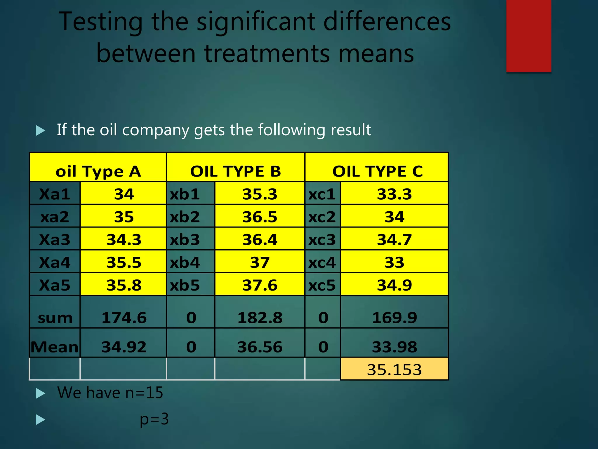
 If the oil company gets the following result
 We have n=15
 p=3
Xa1 34 xb1 35.3 xc1 33.3
xa2 35 xb2 36.5 xc2 34
Xa3 34.3 xb3 36.4 xc3 34.7
Xa4 35.5 xb4 37 xc4 33
Xa5 35.8 xb5 37.6 xc5 34.9
sum 174.6 0 182.8 0 169.9
Mean 34.92 0 36.56 0 33.98
35.153
oil Type A OIL TYPE B OIL TYPE C
Step 1: Determine the null hypothesis and
alternative hypothesis
H0: µ1=µ2=µ3
Ha: at least two of µ1,µ2,µ3 differ
Compare the between-treatment
variability to the within-treatment
variability
 Between-treatment variability is the variability
of the sample means, sample to sample
 Within-treatment variability is the variability of
the treatments (that is, the values) within each
sample
 Step 2 in order to numerically compare
between within and between treatments
variability we define sum of square and
mean square
The treatment sum of
square(SST):measure the variability of the
sample treatment means.
SST=
so 5(34-35.153)+5(36.6-53.153)+5(33.98-35.153)
=17.0493
 

p
i
ii xxn
1
2
2
2 2
 STEP 2 : THE ERROR SUM OF SQUARES
(SSE) measure the within treatment
variability
SSE=
We compute the SSE by calculating the
squared difference between each observed
value.
So [(34.0-34.92)+(35-34.92)+…….+(34.9-
33.98)]
=8.028
  

p
i
n
j
iij
i
xx
1 1
2
22 2
 Step 3 we define a sum of square that measures
the total amount of variability in the observed
values of the response. The total sum of square
SSTO
SSTO=SST+SSE
17.0493+8.028=25.0773
 Using the treatment and error sums of square we
next define two mean square:
 The treatment mean square is MST=SST/P-1
17.0493/3-1
8.525
 The error mean square is MSE=SSE/n-p
8.028/15-3
0.669
 THEN WE CALCULATE F VALUE
DEFINE F statistic
And its value to the area under the F curve with
p-1 and n-p degree of freedom to the right of F.
We reject H0 at the significance a if either of
the following conditions holds
1. F>Fa 2. p-value <a
 
   11
1
:StatisticTest


bp-SSE/
p-SST/
MSE
MST
F=
 IT FOLLOWS THAT
F=8.525/0.669=12.74
IN order to test H0 at the 0.05 level of
significance we use F .05 with p-1 =3-1=2
nominator and n-p=15-3=12 denominator,
From the table we got 3.89
So we have F=12.74>F .05=3.89
There fore, we reject H0 at the 0.05 level of
significance.
In other words we conclude that at least two of
oil types A B C have different effects on the
mean mileage.
Pairwise comparison
 If one way anova f test says that at least two treatment
mean differ, we estimate how large the difference are.
 Comparing treatment means two at a time.
 In our example we might estimate the pairwise
differences µa-µb, it is the change in mean mileage
achieved by changeling from B to A
 There are two approaches to calculating intervals for
pairwise differences
1. INDIVIDUAL: the confidence interval for each
pairwise difference
ta/2 is based on n – p degrees of freedom
  






hi
α/hi
nn
MSEtxx
11
2
2. Simultaneous confidence interval : such an
interval make us 100(1-a) percent
confidence that all of the pairwise difference
are simultaneously contained in their
respective intervals. There are so many kinds
but mostly Tukey formula used.
qa is the upper a percentage point of the
studentized range for p and (n – p) from
Table
 
m
MSE
qxx αhi 
 E.g in the oil mileage example we are
comparing
p=3 treatments
each sample size m=5 total n=15
MSE=0.669 q.05=3.77 from the table
corresponding to p=3 and n-p=12
Similar Tukey simultaneous 95 % confidence
interval for µb-µa
[(36.56-34.92)±3.77 0.669/5=
[0.261,3.019]
The interval make us simultaneously 95%
confidence that 1 changing from oil type A to oil
B increase mean mileage by between 02.61 and
3.019 mpg.

Anova ONE WAY

  • 1.
  • 2.
     IT USEDTO ESTIMATE AND COMPARE THE EFFECTES OF THE Difference treatments on the response variables  We do this by estimating and comparing the treatments means  When we compare more than two groups based on one factors. E.g. If one the car oil company would to like to compare the effects of three oil type assume that A,B and C on oil mileage by midsize cars. And the company select randomly 5 cars from 1000 cars. There is only one Factor : oil type
  • 3.
    Assumptions on oneway ANOVA 1. Constant variance: the populations of values of the response variable associated with the treatments have equal variables. 2. Normality: the pupations of the values of the response variable associated with the treatments all have normal distributions 3. Independence: the samples of experimental units associated with the treatments are randomly selected, independent sample
  • 4.
    Testing the significantdifferences between treatments means  If the oil company gets the following result  We have n=15  p=3 Xa1 34 xb1 35.3 xc1 33.3 xa2 35 xb2 36.5 xc2 34 Xa3 34.3 xb3 36.4 xc3 34.7 Xa4 35.5 xb4 37 xc4 33 Xa5 35.8 xb5 37.6 xc5 34.9 sum 174.6 0 182.8 0 169.9 Mean 34.92 0 36.56 0 33.98 35.153 oil Type A OIL TYPE B OIL TYPE C
  • 5.
    Step 1: Determinethe null hypothesis and alternative hypothesis H0: µ1=µ2=µ3 Ha: at least two of µ1,µ2,µ3 differ Compare the between-treatment variability to the within-treatment variability  Between-treatment variability is the variability of the sample means, sample to sample  Within-treatment variability is the variability of the treatments (that is, the values) within each sample
  • 6.
     Step 2in order to numerically compare between within and between treatments variability we define sum of square and mean square The treatment sum of square(SST):measure the variability of the sample treatment means. SST= so 5(34-35.153)+5(36.6-53.153)+5(33.98-35.153) =17.0493    p i ii xxn 1 2 2 2 2
  • 7.
     STEP 2: THE ERROR SUM OF SQUARES (SSE) measure the within treatment variability SSE= We compute the SSE by calculating the squared difference between each observed value. So [(34.0-34.92)+(35-34.92)+…….+(34.9- 33.98)] =8.028     p i n j iij i xx 1 1 2 22 2
  • 8.
     Step 3we define a sum of square that measures the total amount of variability in the observed values of the response. The total sum of square SSTO SSTO=SST+SSE 17.0493+8.028=25.0773  Using the treatment and error sums of square we next define two mean square:  The treatment mean square is MST=SST/P-1 17.0493/3-1 8.525  The error mean square is MSE=SSE/n-p 8.028/15-3 0.669
  • 9.
     THEN WECALCULATE F VALUE DEFINE F statistic And its value to the area under the F curve with p-1 and n-p degree of freedom to the right of F. We reject H0 at the significance a if either of the following conditions holds 1. F>Fa 2. p-value <a      11 1 :StatisticTest   bp-SSE/ p-SST/ MSE MST F=
  • 10.
     IT FOLLOWSTHAT F=8.525/0.669=12.74 IN order to test H0 at the 0.05 level of significance we use F .05 with p-1 =3-1=2 nominator and n-p=15-3=12 denominator, From the table we got 3.89 So we have F=12.74>F .05=3.89 There fore, we reject H0 at the 0.05 level of significance. In other words we conclude that at least two of oil types A B C have different effects on the mean mileage.
  • 11.
    Pairwise comparison  Ifone way anova f test says that at least two treatment mean differ, we estimate how large the difference are.  Comparing treatment means two at a time.  In our example we might estimate the pairwise differences µa-µb, it is the change in mean mileage achieved by changeling from B to A  There are two approaches to calculating intervals for pairwise differences 1. INDIVIDUAL: the confidence interval for each pairwise difference ta/2 is based on n – p degrees of freedom          hi α/hi nn MSEtxx 11 2
  • 12.
    2. Simultaneous confidenceinterval : such an interval make us 100(1-a) percent confidence that all of the pairwise difference are simultaneously contained in their respective intervals. There are so many kinds but mostly Tukey formula used. qa is the upper a percentage point of the studentized range for p and (n – p) from Table   m MSE qxx αhi 
  • 13.
     E.g inthe oil mileage example we are comparing p=3 treatments each sample size m=5 total n=15 MSE=0.669 q.05=3.77 from the table corresponding to p=3 and n-p=12 Similar Tukey simultaneous 95 % confidence interval for µb-µa [(36.56-34.92)±3.77 0.669/5= [0.261,3.019] The interval make us simultaneously 95% confidence that 1 changing from oil type A to oil B increase mean mileage by between 02.61 and 3.019 mpg.

Editor's Notes