This document provides information about independent samples t-tests and dependent/paired samples t-tests. It explains that independent samples t-tests are used to compare two independent groups, while dependent samples t-tests are used to compare observations within a single group. The key steps for each test are outlined, including stating hypotheses, calculating the test statistic, determining critical values, and making conclusions. Examples are provided to demonstrate how to perform the tests by hand and using SPSS.

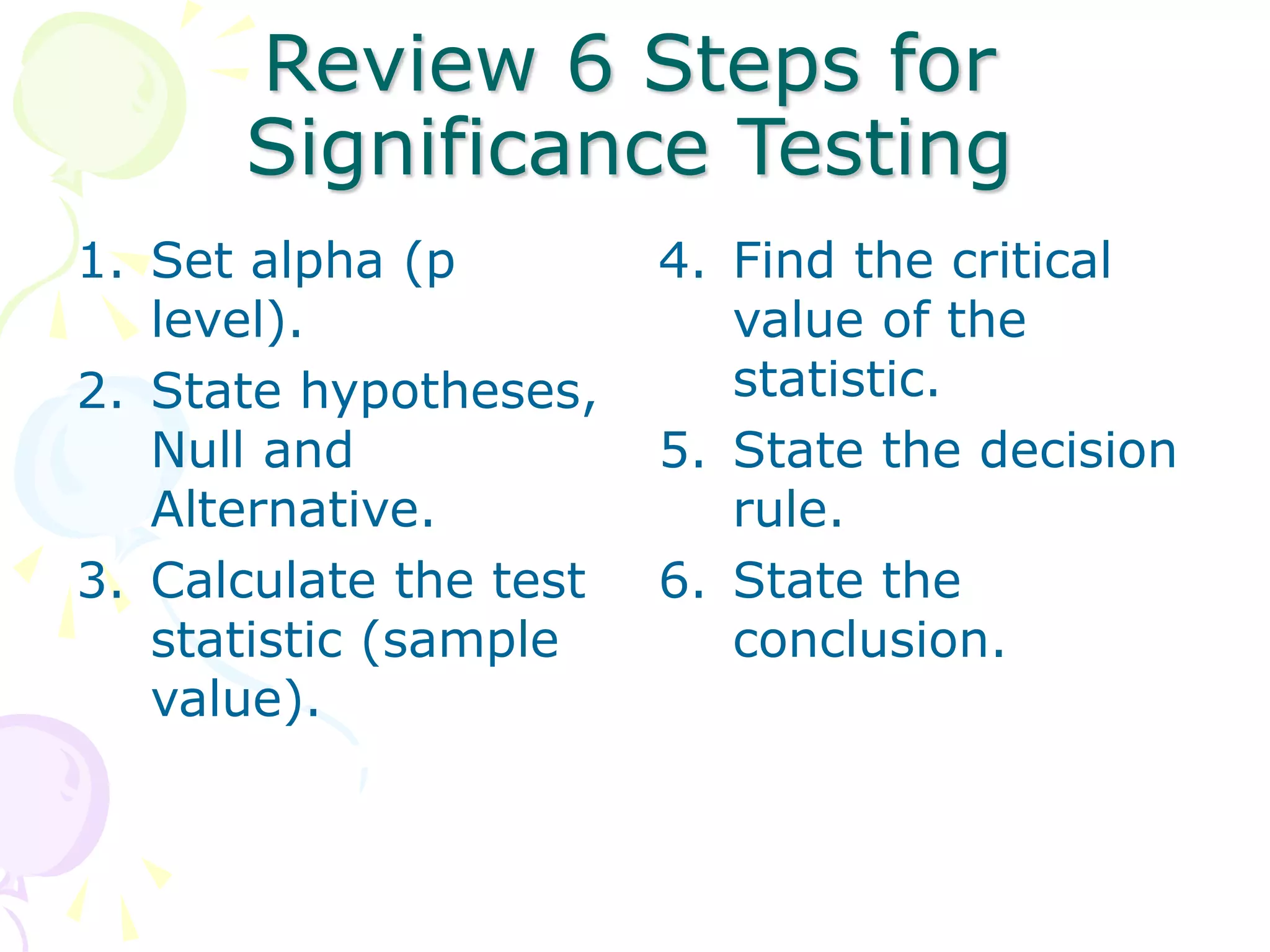
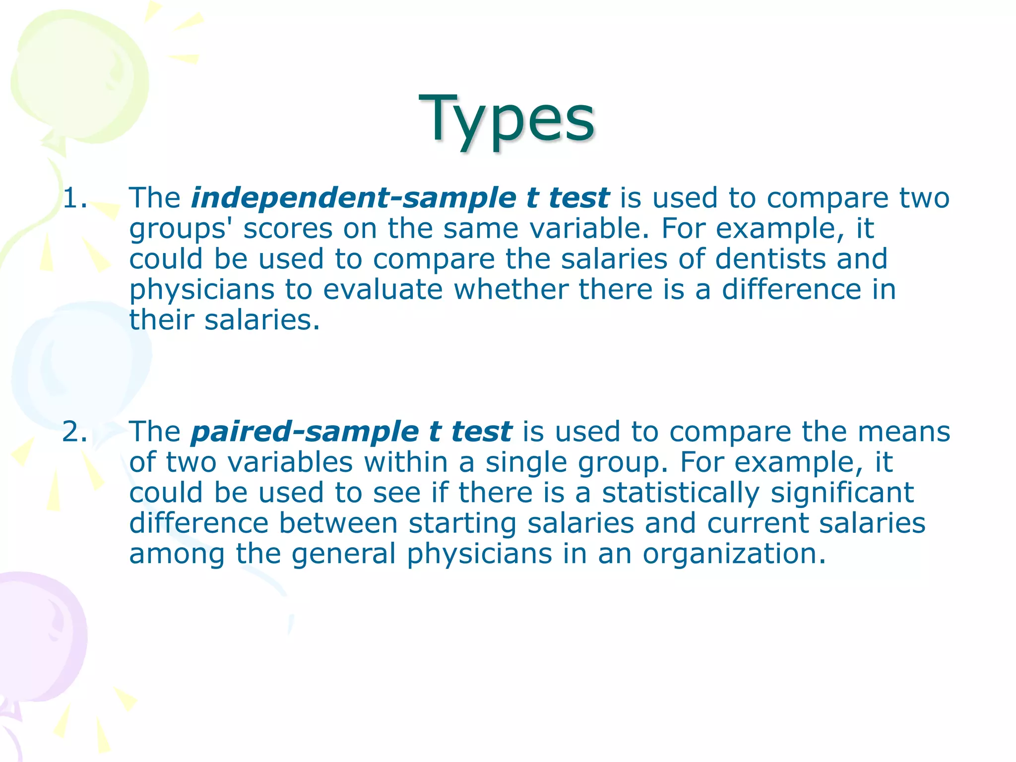
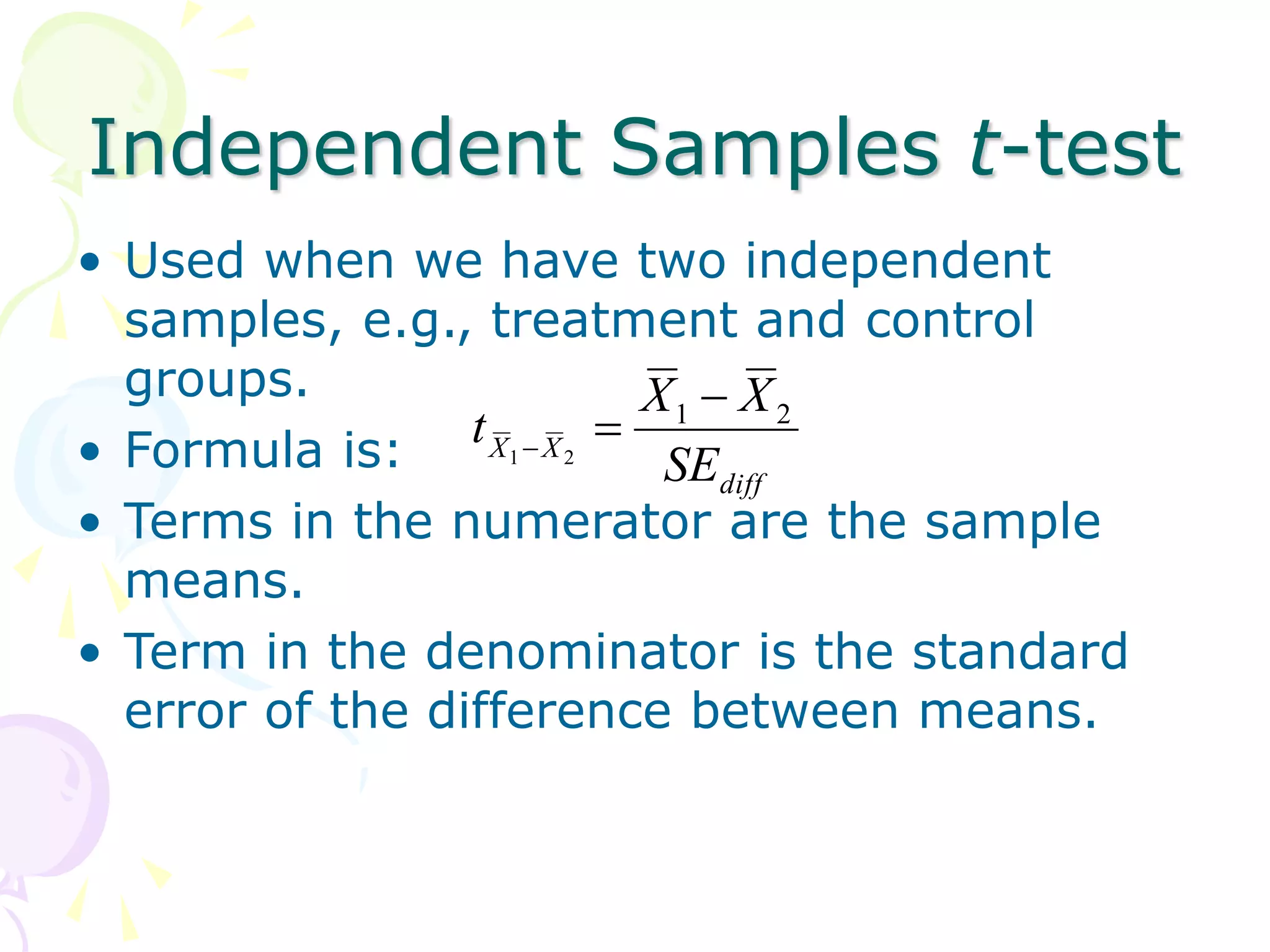
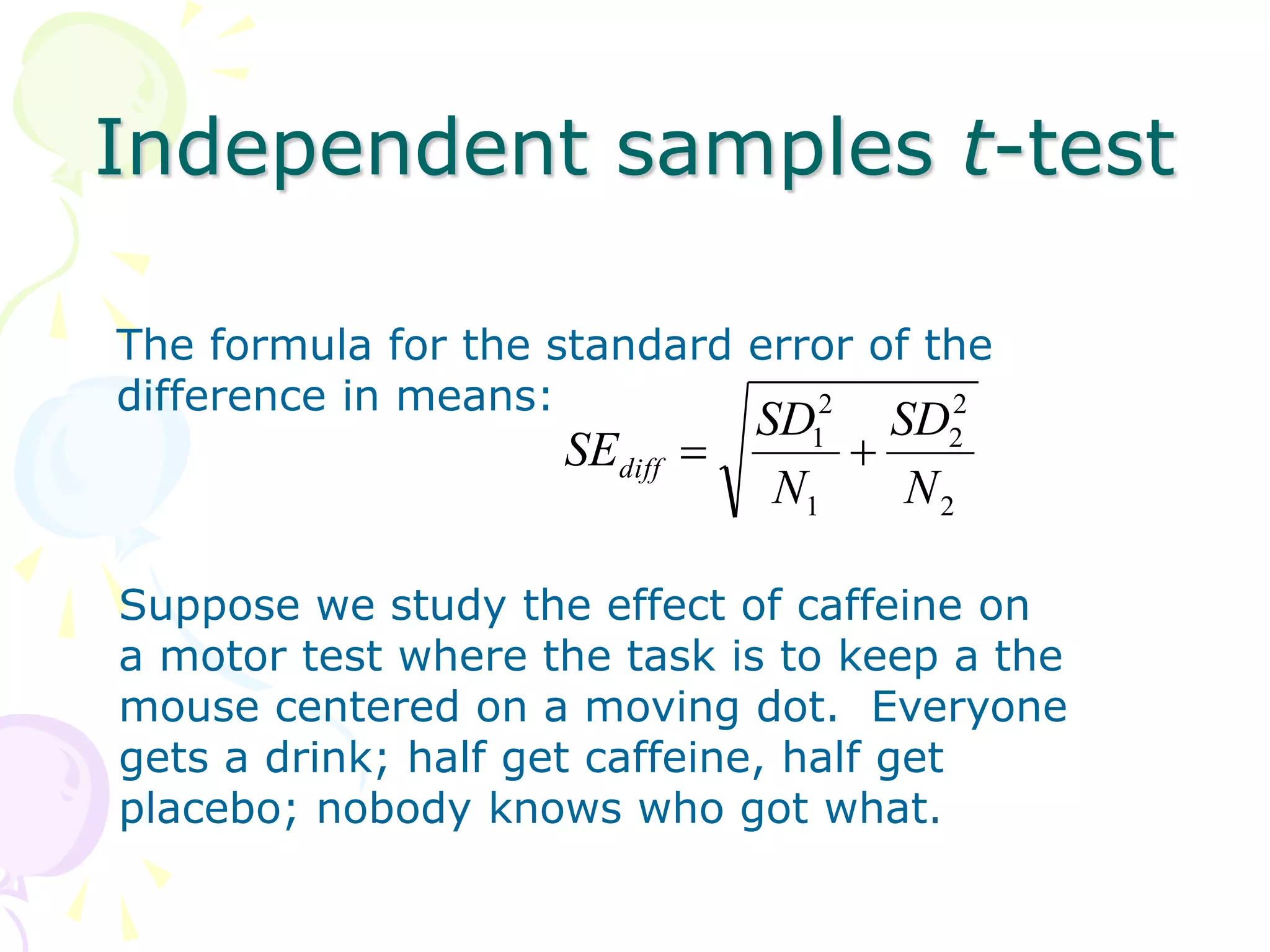
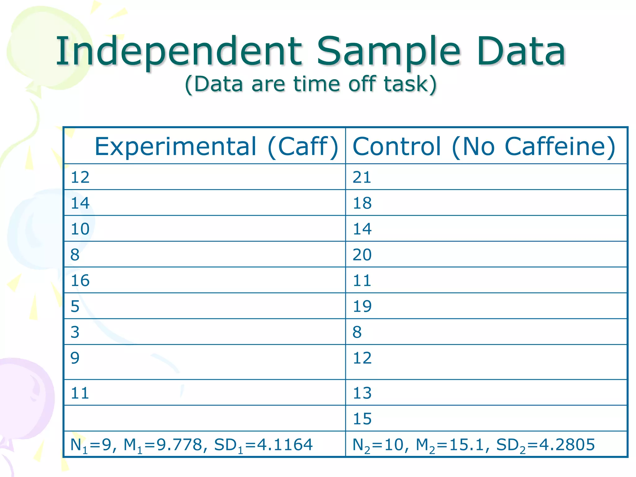
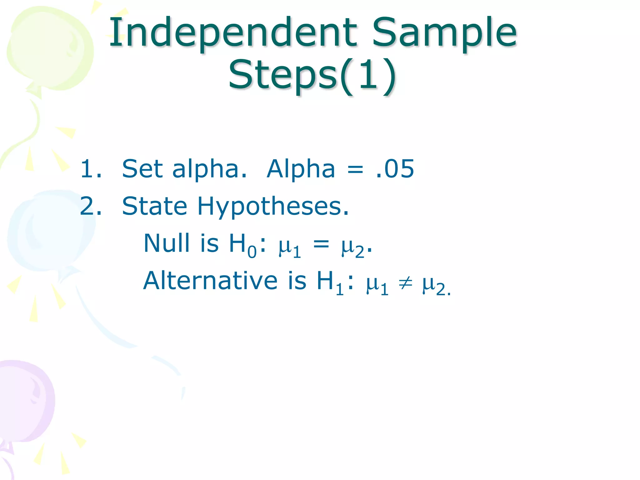
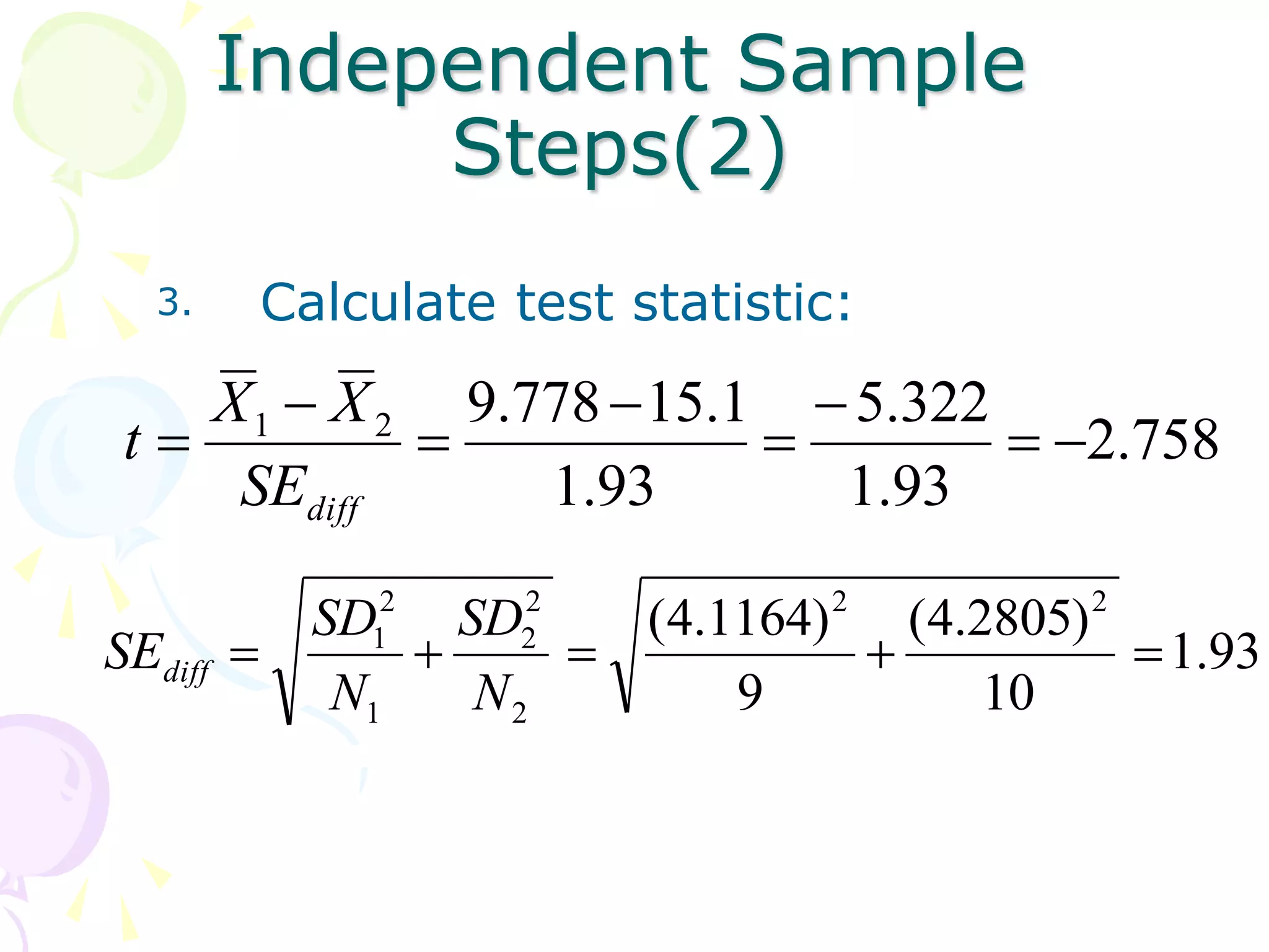
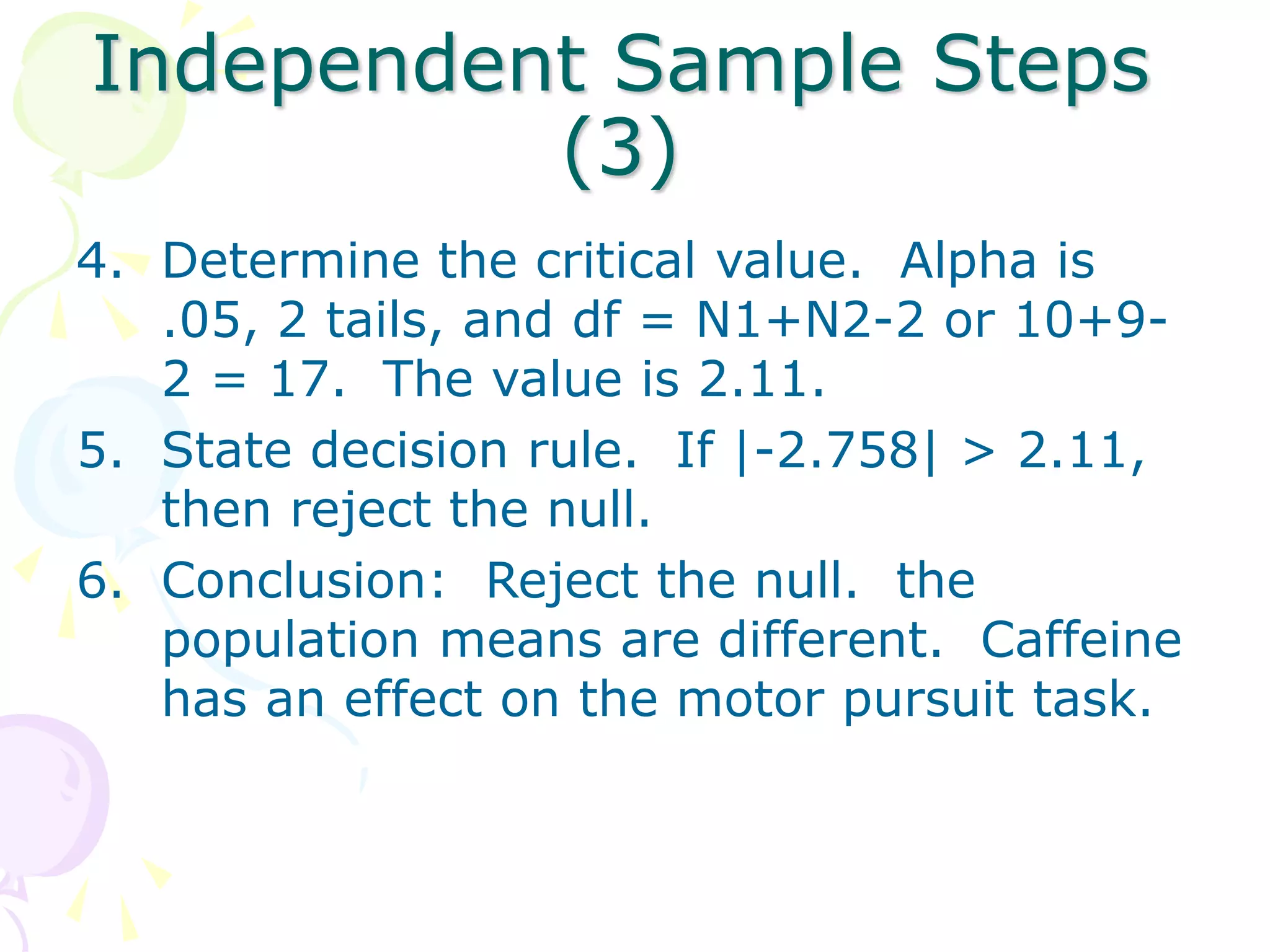
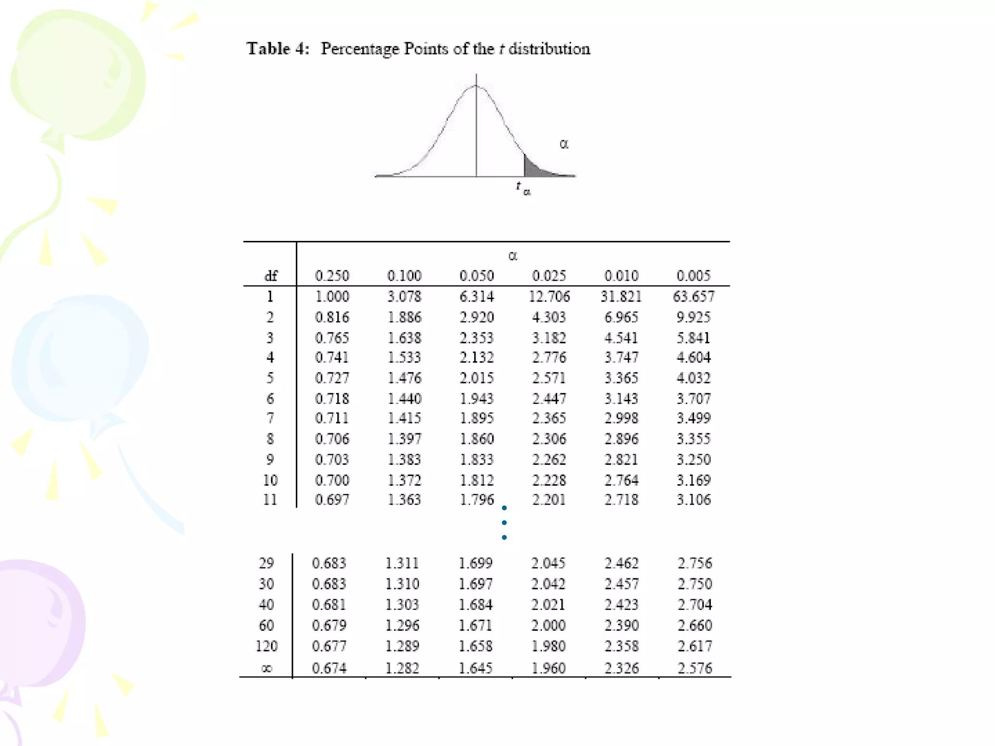
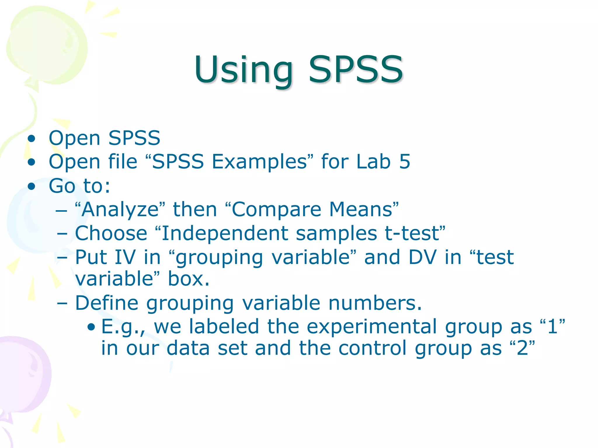
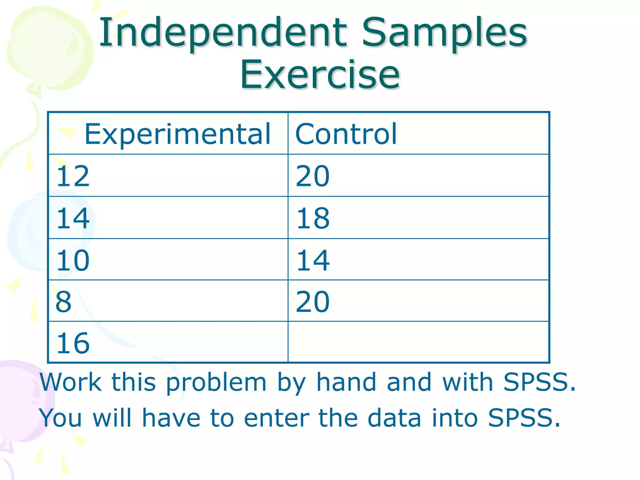
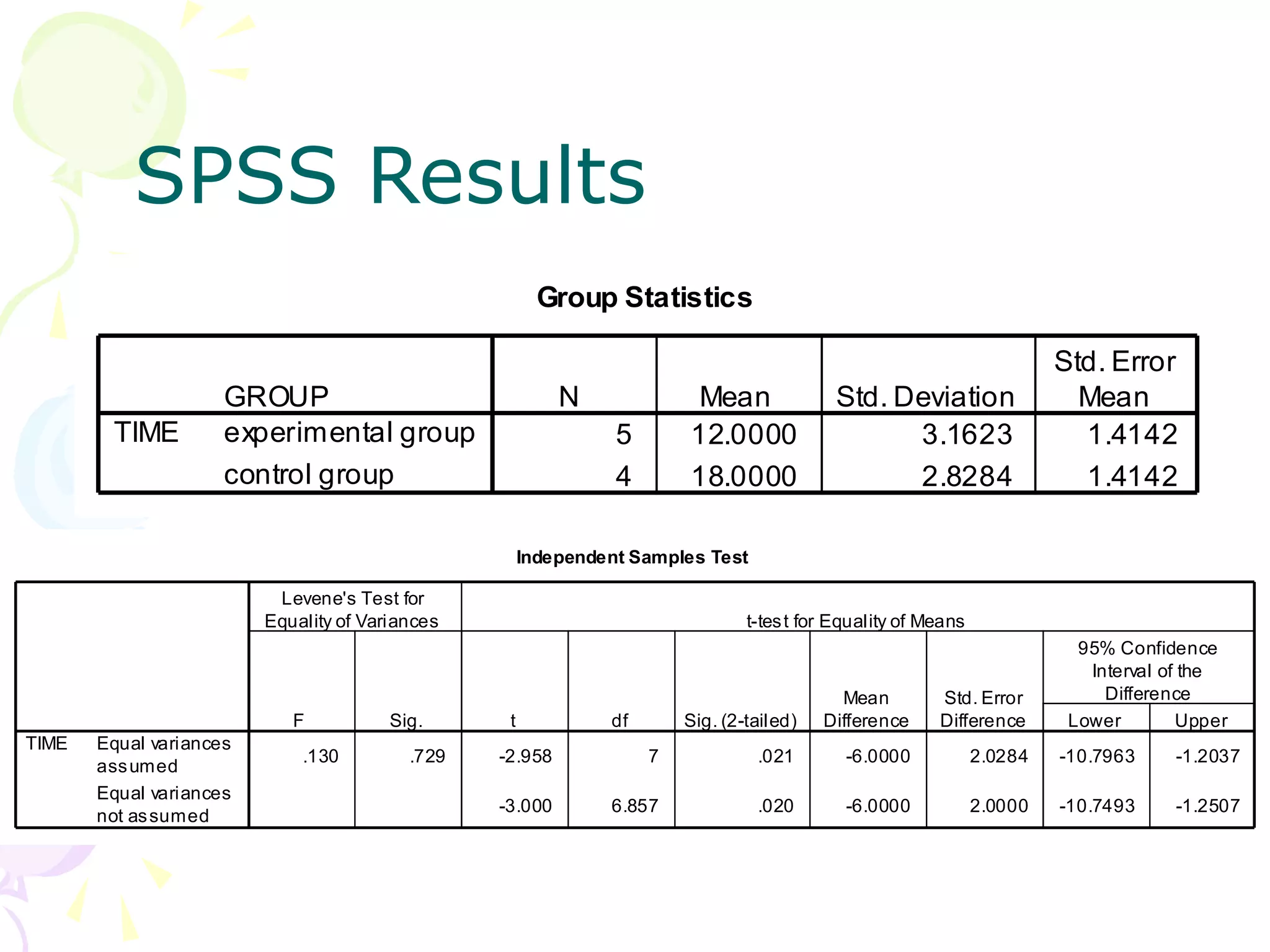
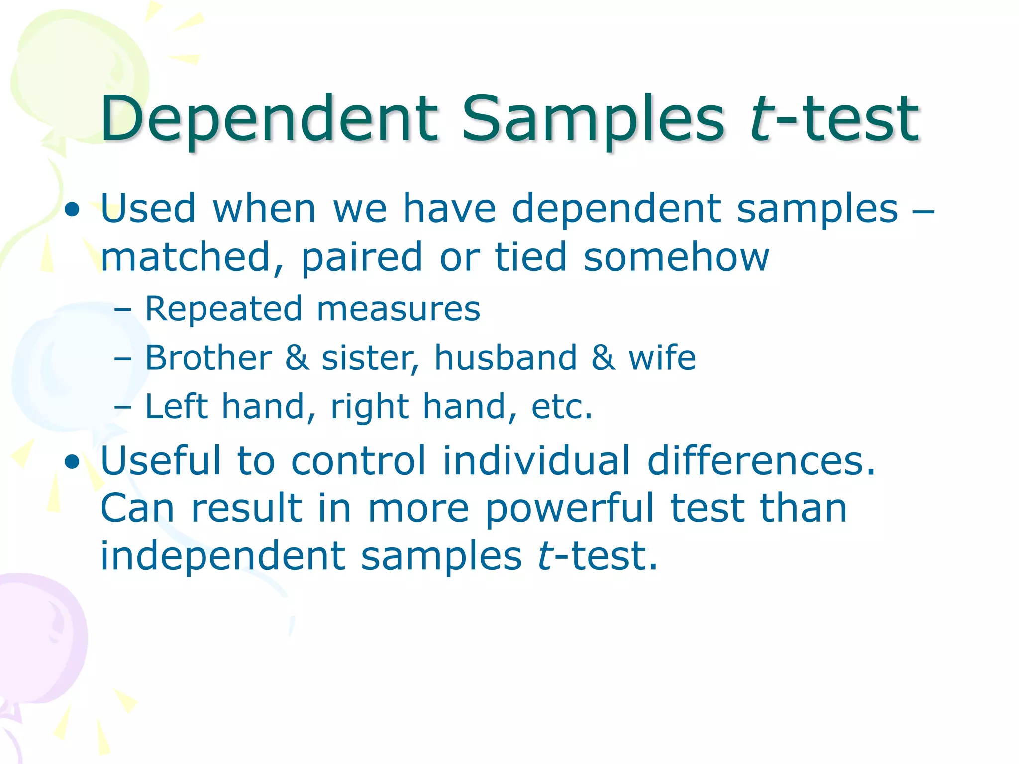
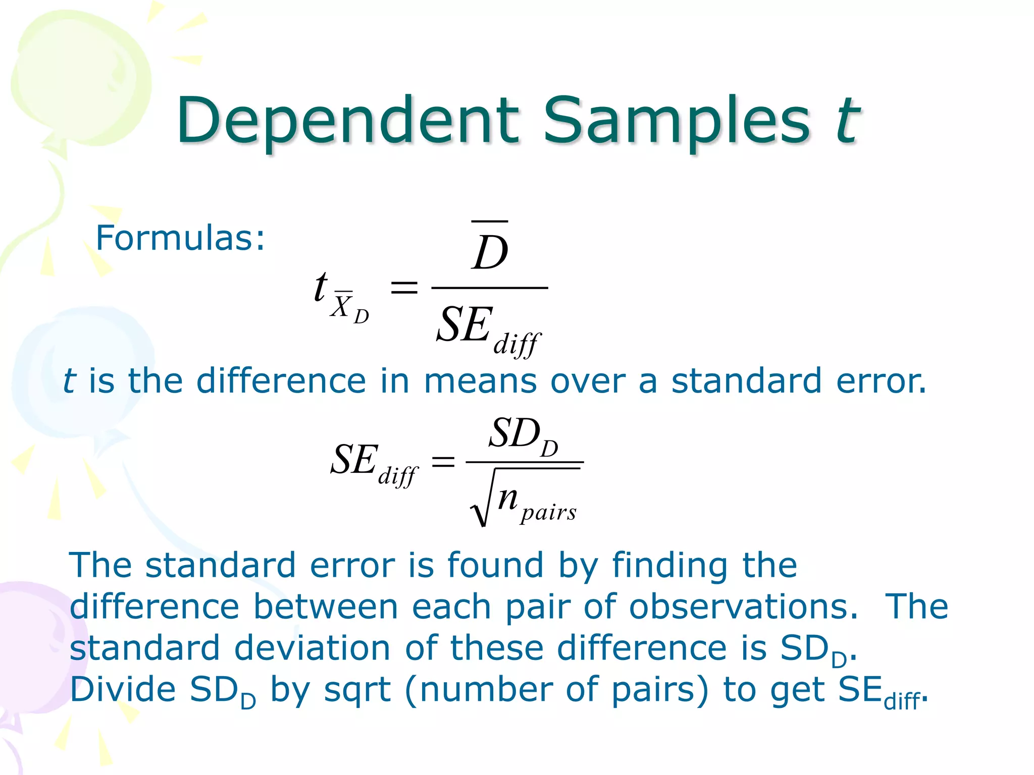
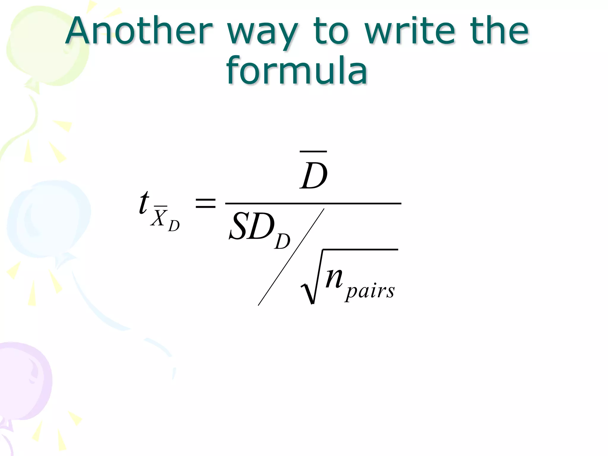
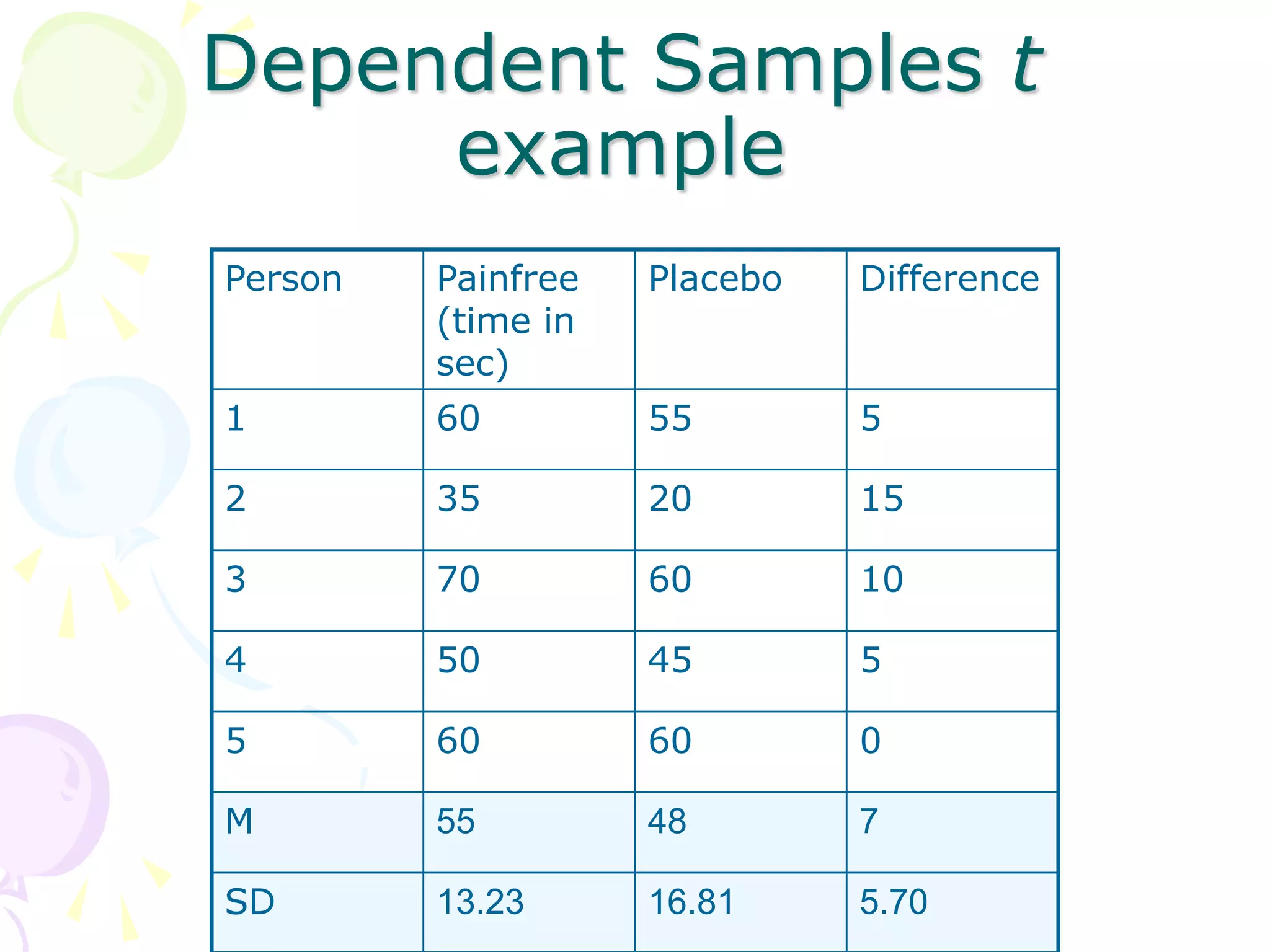
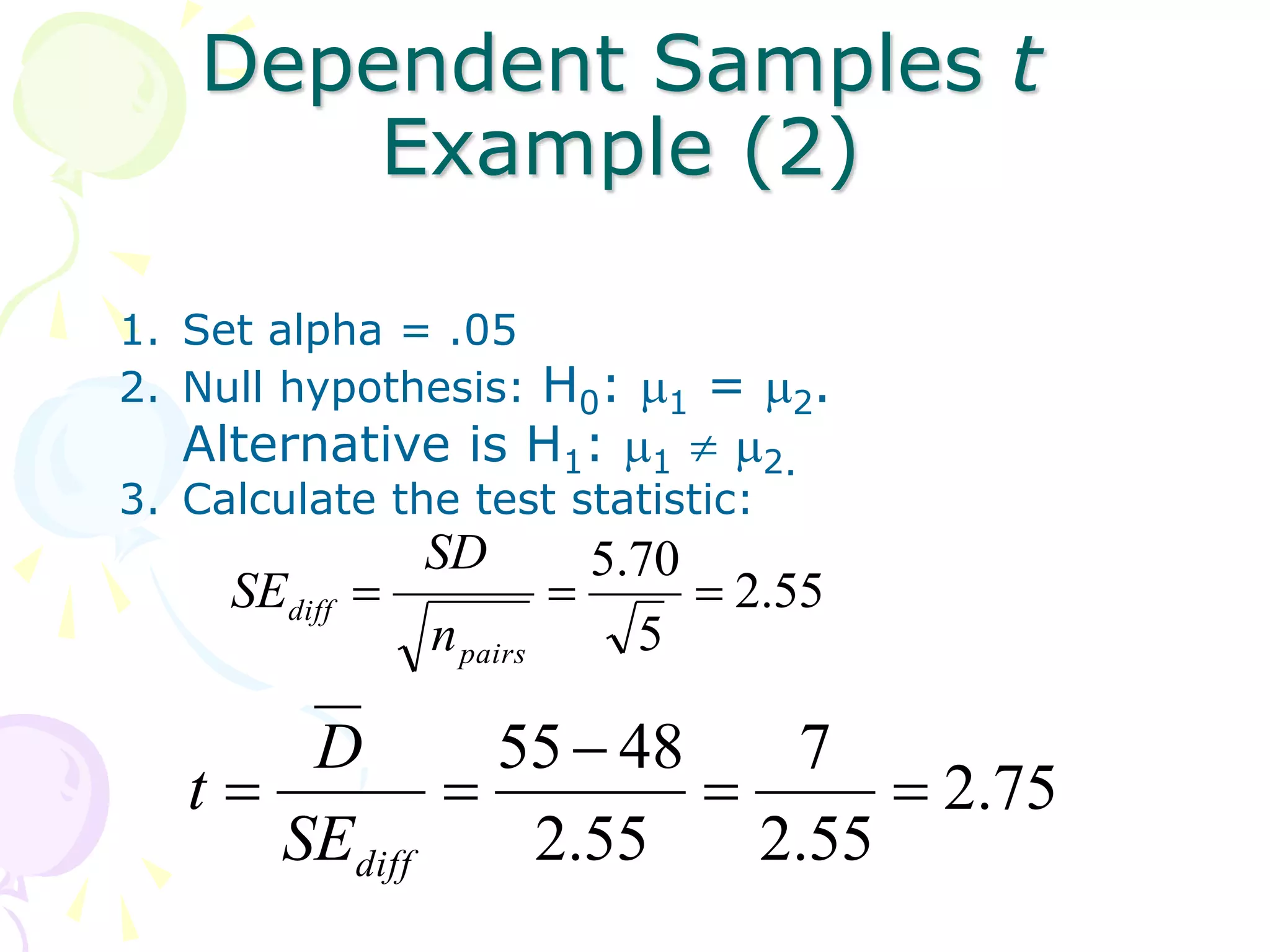
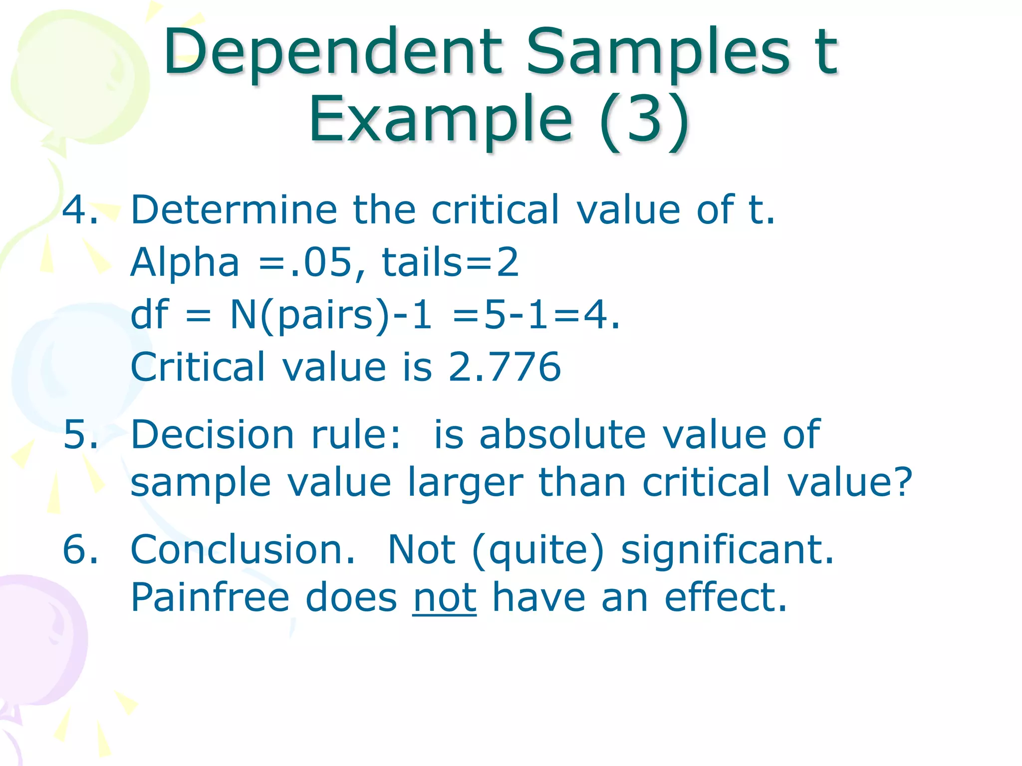
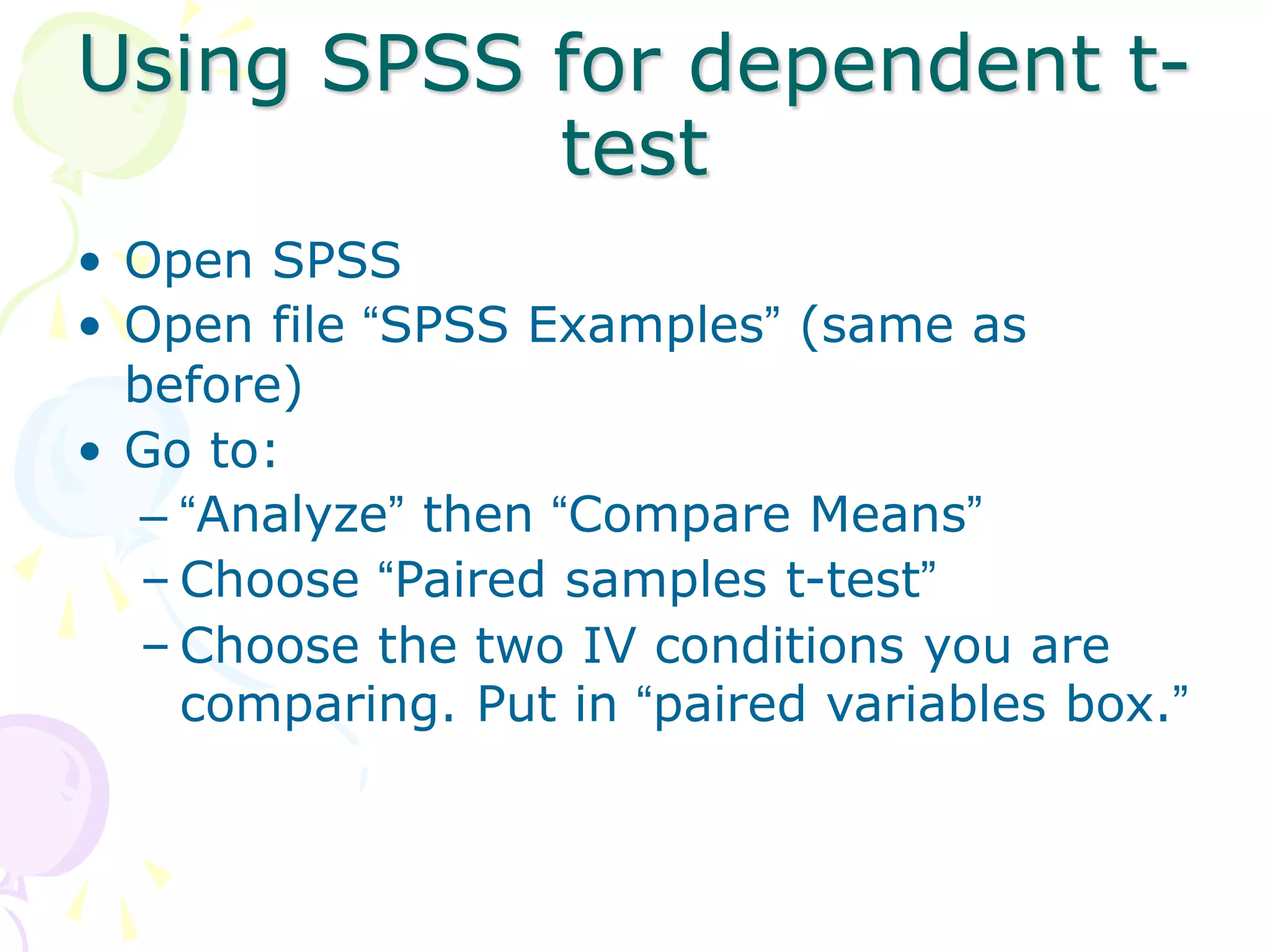
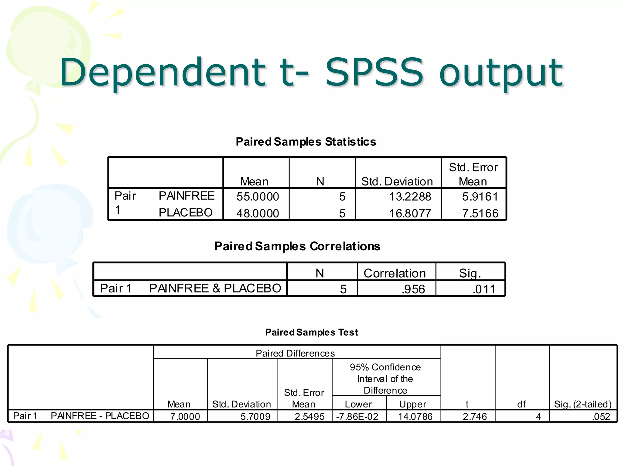
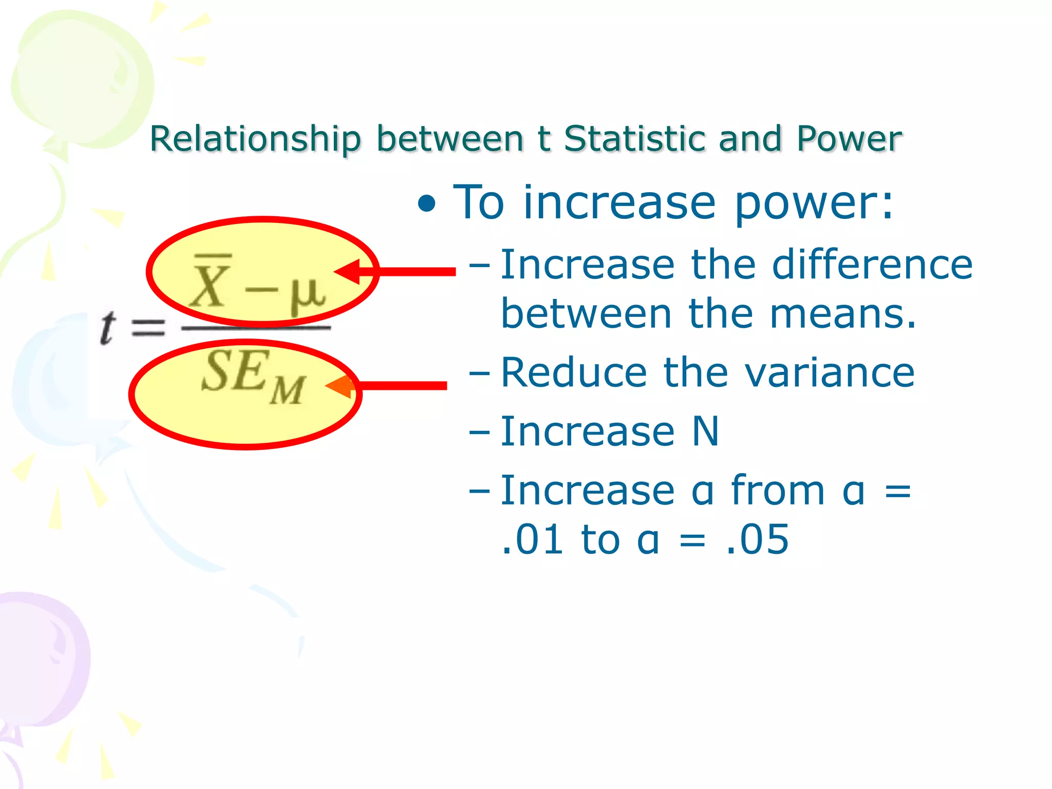
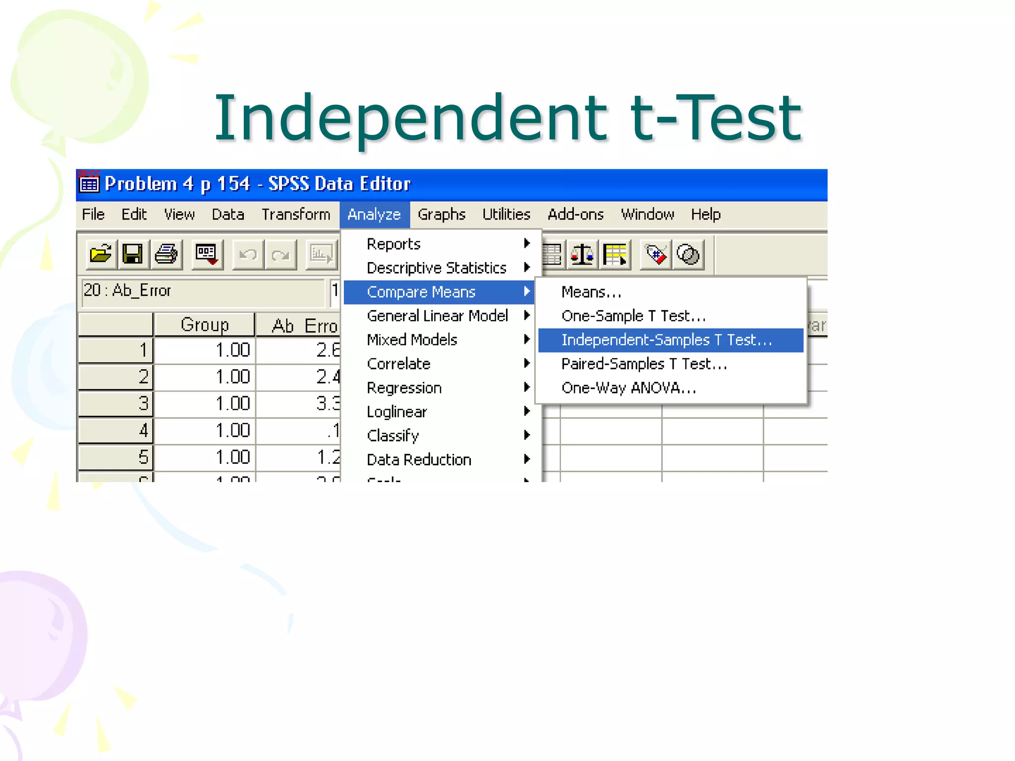
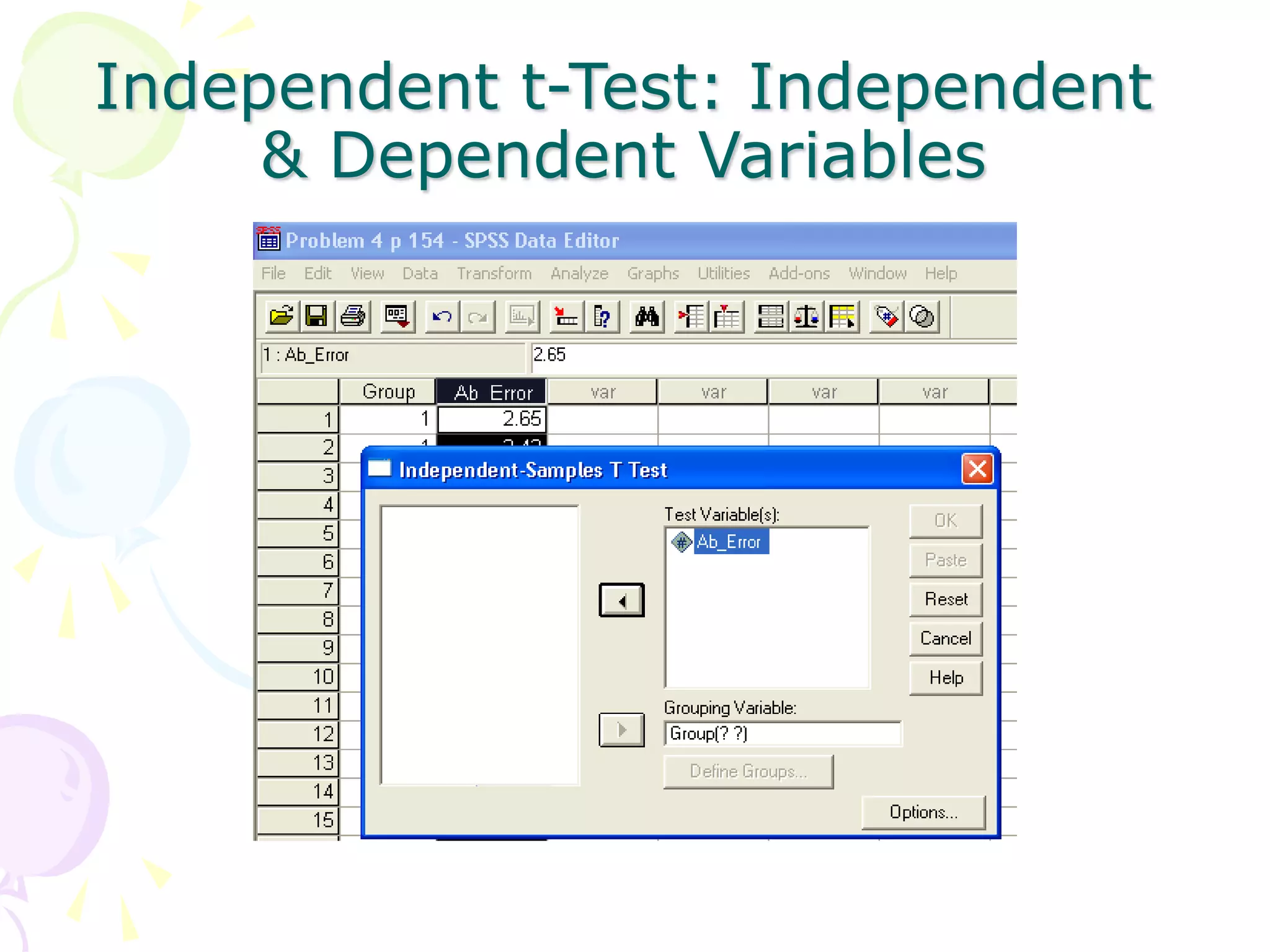
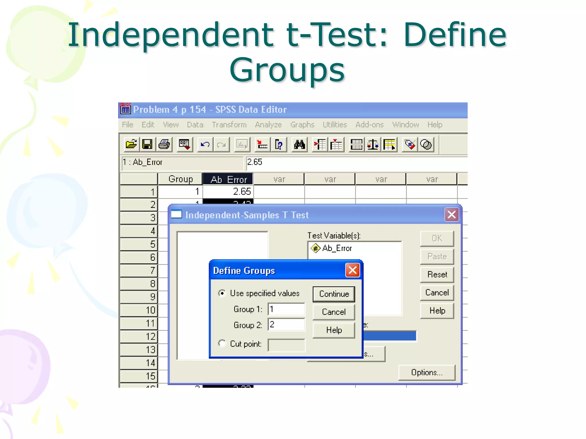
1. t-test
Dr. Hamza Aduraidi

2. Review 6 Steps for
Significance Testing
1. Set alpha (p
level).
2. State hypotheses,
Null and
Alternative.
3. Calculate the test
statistic (sample
value).
4. Find the critical
value of the
statistic.
5. State the decision
rule.
6. State the
conclusion.

3. t-test
• t –test is about means: distribution and
evaluation for group distribution
• Withdrawn form the normal distribution
• The shape of distribution depend on
sample size and, the sum of all
distributions is a normal distribution
• t- distribution is based on sample size and
vary according to the degrees of freedom

4. What is the t -test
• t test is a useful technique for comparing
mean values of two sets of numbers.
• The comparison will provide you with a
statistic for evaluating whether the difference
between two means is statistically significant.
• t test is named after its inventor, William
Gosset, who published under the pseudonym
of student.
• t test can be used either :
1.to compare two independent groups (independent-
samples t test)
2.to compare observations from two measurement
occasions for the same group (paired-samples t
test).

5. What is the t -test
• The null hypothesis states that any
difference between the two means is a
result to difference in distribution.
• Remember, both samples drawn randomly
form the same population.
• Comparing the chance of having difference
is one group due to difference in
distribution.
• Assuming that both distributions
came from the same population, both
distribution has to be equal.

6. What is the t -test
• Then, what we intend:
“To find the difference due to chance”
• Logically, The larger the difference in means, the
more likely to find a significant t test.
• But, recall:
1.Variability
More variability = less overlap = larger difference
2. Sample size
Larger sample size = less variability (pop) = larger difference

7. Types
1. The independent-sample t test is used to compare two
groups' scores on the same variable. For example, it
could be used to compare the salaries of dentists and
physicians to evaluate whether there is a difference in
their salaries.
2. The paired-sample t test is used to compare the means
of two variables within a single group. For example, it
could be used to see if there is a statistically significant
difference between starting salaries and current salaries
among the general physicians in an organization.

8. Assumption
1. Dependent variable should be
continuous (I/R)
2. The groups should be randomly
drawn from normally distributed
and independent populations
e.g. Male X Female
Dentist X Physician
Manager X Staff
NO OVER LAP

9. Assumption
3. the independent variable is categorical with two
levels
4. Distribution for the two independent variables
is normal
5. Equal variance (homogeneity of variance)
6. large variation = less likely to have sig t test =
accepting null hypothesis (fail to reject) = Type
II error = a threat to power
Sending an innocent to jail for no significant reason

10. Independent Samples t-test
• Used when we have two independent
samples, e.g., treatment and control
groups.
• Formula is:
• Terms in the numerator are the sample
means.
• Term in the denominator is the standard
error of the difference between means.
diff
X
X
SE
X
X
t 2
1
2
1




11. Independent samples t-test
The formula for the standard error of the
difference in means:
2
2
2
1
2
1
N
SD
N
SD
SEdiff 

Suppose we study the effect of caffeine on
a motor test where the task is to keep a the
mouse centered on a moving dot. Everyone
gets a drink; half get caffeine, half get
placebo; nobody knows who got what.

12. Independent Sample Data
(Data are time off task)
Experimental (Caff) Control (No Caffeine)
12 21
14 18
10 14
8 20
16 11
5 19
3 8
9 12
11 13
15
N1=9, M1=9.778, SD1=4.1164 N2=10, M2=15.1, SD2=4.2805

13. Independent Sample
Steps(1)
1. Set alpha. Alpha = .05
2. State Hypotheses.
Null is H0: 1 = 2.
Alternative is H1: 1  2.

14. Independent Sample
Steps(2)
3. Calculate test statistic:
93
.
1
10
)
2805
.
4
(
9
)
1164
.
4
( 2
2
2
2
2
1
2
1





N
SD
N
SD
SEdiff
758
.
2
93
.
1
322
.
5
93
.
1
1
.
15
778
.
9
2
1








diff
SE
X
X
t

15. Independent Sample Steps
(3)
4. Determine the critical value. Alpha is
.05, 2 tails, and df = N1+N2-2 or 10+9-
2 = 17. The value is 2.11.
5. State decision rule. If |-2.758| > 2.11,
then reject the null.
6. Conclusion: Reject the null. the
population means are different. Caffeine
has an effect on the motor pursuit task.

16. …

17. Using SPSS
• Open SPSS
• Open file “SPSS Examples” for Lab 5
• Go to:
– “Analyze” then “Compare Means”
– Choose “Independent samples t-test”
– Put IV in “grouping variable” and DV in “test
variable” box.
– Define grouping variable numbers.
• E.g., we labeled the experimental group as “1”
in our data set and the control group as “2”

18. Independent Samples
Exercise
Experimental Control
12 20
14 18
10 14
8 20
16
Work this problem by hand and with SPSS.
You will have to enter the data into SPSS.

19. Group Statistics
5 12.0000 3.1623 1.4142
4 18.0000 2.8284 1.4142
GROUP
experimental group
control group
TIME
N Mean Std. Deviation
Std. Error
Mean
Independent Samples Test
.130 .729 -2.958 7 .021 -6.0000 2.0284 -10.7963 -1.2037
-3.000 6.857 .020 -6.0000 2.0000 -10.7493 -1.2507
Equal variances
assumed
Equal variances
not assumed
TIME
F Sig.
Levene's Test for
Equality of Variances
t df Sig. (2-tailed)
Mean
Difference
Std. Error
Difference Lower Upper
95% Confidence
Interval of the
Difference
t-test for Equality of Means
SPSS Results

20. Dependent
Samples
t-tests

21. Dependent Samples t-test
• Used when we have dependent samples –
matched, paired or tied somehow
– Repeated measures
– Brother & sister, husband & wife
– Left hand, right hand, etc.
• Useful to control individual differences.
Can result in more powerful test than
independent samples t-test.

22. Dependent Samples t
Formulas:
diff
X
SE
D
t D

t is the difference in means over a standard error.
pairs
D
diff
n
SD
SE 
The standard error is found by finding the
difference between each pair of observations. The
standard deviation of these difference is SDD.
Divide SDD by sqrt (number of pairs) to get SEdiff.

23. Another way to write the
formula
pairs
D
X
n
SD
D
t D


24. Dependent Samples t
example
Person Painfree
(time in
sec)
Placebo Difference
1 60 55 5
2 35 20 15
3 70 60 10
4 50 45 5
5 60 60 0
M 55 48 7
SD 13.23 16.81 5.70

25. Dependent Samples t
Example (2)
55
.
2
5
70
.
5



pairs
diff
n
SD
SE
75
.
2
55
.
2
7
55
.
2
48
55





diff
SE
D
t
1. Set alpha = .05
2. Null hypothesis: H0: 1 = 2.
Alternative is H1: 1  2.
3. Calculate the test statistic:

26. Dependent Samples t
Example (3)
4. Determine the critical value of t.
Alpha =.05, tails=2
df = N(pairs)-1 =5-1=4.
Critical value is 2.776
5. Decision rule: is absolute value of
sample value larger than critical value?
6. Conclusion. Not (quite) significant.
Painfree does not have an effect.

27. Using SPSS for dependent t-
test
• Open SPSS
• Open file “SPSS Examples” (same as
before)
• Go to:
– “Analyze” then “Compare Means”
– Choose “Paired samples t-test”
– Choose the two IV conditions you are
comparing. Put in “paired variables box.”

28. Dependent t- SPSS output
Paired Samples Statistics
55.0000 5 13.2288 5.9161
48.0000 5 16.8077 7.5166
PAINFREE
PLACEBO
Pair
1
Mean N Std. Deviation
Std. Error
Mean
Paired Samples Correlations
5 .956 .011
PAINFREE & PLACEBO
Pair 1
N Correlation Sig.
Paired Samples Test
7.0000 5.7009 2.5495 -7.86E-02 14.0786 2.746 4 .052
PAINFREE - PLACEBO
Pair 1
Mean Std. Deviation
Std. Error
Mean Lower Upper
95% Confidence
Interval of the
Difference
Paired Differences
t df Sig. (2-tailed)

29. Relationship between t Statistic and Power
• To increase power:
– Increase the difference
between the means.
– Reduce the variance
– Increase N
– Increase α from α =
.01 to α = .05

30. To Increase Power
• Increase alpha, Power for α = .10 is
greater than power for α = .05
• Increase the difference between
means.
• Decrease the sd’s of the groups.
• Increase N.

31. Independent t-Test

32. Independent t-Test: Independent
& Dependent Variables

33. Independent t-Test: Define
Groups

34. Independent t-Test: Options

35. Independent t-Test:
Output
Group Statistics
10 2.2820 1.24438 .39351
10 1.9660 1.50606 .47626
Group
Active
Passive
Ab_Error
N Mean Std. Deviation
Std. Error
Mean
Independent Samples Test
.513 .483 .511 18 .615 .31600 .61780 -.98194 1.61394
.511 17.382 .615 .31600 .61780 -.98526 1.61726
Equal variances
assumed
Equal variances
not assumed
Ab_Error
F Sig.
Levene's Test for
Equality of Variances
t df Sig. (2-tailed)
Mean
Difference
Std. Error
Difference Lower Upper
95% Confidence
Interval of the
Difference
t-test for Equality of Means
Are the groups
different?
t(18) = .511, p = .615
NO DIFFERENCE
2.28 is not different
from 1.96

36. Dependent or Paired t-Test: Define
Variables

37. Dependent or Paired t-Test: Select
Paired-Samples

38. Dependent or Paired t-Test: Select
Variables

39. Dependent or Paired t-Test: Options

40. Dependent or Paired
t-Test: Output
PairedSamples Statistics
4.7000 10 2.11082 .66750
6.2000 10 2.85968 .90431
Pre
Post
Pair
1
Mean N Std. Deviation
Std. Error
Mean
Paired Samples Correlations
10 .968 .000
Pre & Post
Pair 1
N Correlation Sig.
Paired Samples Test
-1.50000 .97183 .30732 -2.19520 -.80480 -4.881 9 .001
Pre - Post
Pair 1
Mean Std. Deviation
Std. Error
Mean Lower Upper
95% Confidence
Interval of the
Difference
Paired Differences
t df Sig. (2-tailed)
Is there a difference between pre & post?
t(9) = -4.881, p = .001
Yes, 4.7 is significantly different from 6.2