1. COLLEGE OF ENGINEERING Civil & Construction Engineering
WAVE GENERATION STUDY OF A 3-D WAVE BASIN
Periodic Wave Generation
Sinusoidal motions of the wave paddles with
prescribed frequency and period are used to
generate periodic waves. Figure 3 shows the water
surface elevation recorded at wave gauge 5 for
wave period = 3s and wave height = 0.221m. 200
waves are generated during the test run.
Periodic Wave Propagation
Measured progressive periodic wave properties vary with
time. Wave gauge records show that the wave profiles vary
at different locations. Using Fourier transform between
four wave gauges along the cross-shore direction, in
addition to the dominant linear waves, two second order
wave components are found:
• Bounded waves propagating with same velocity as the
first order waves (yellow solid lines, Figures 6 and 7).
• Free waves propagating with a slightly slower velocity
than the first order waves (purple solid lines, Figures 6
and 7).
By introducing a secondary motion of the paddles, the
second order free wave can be suppressed. The wave
profile matches better with second-order theory, (Figure
7.)
Introduction
Linear wave generation methods have been used
in wave basins globally. In the O.H. Hinsdale
Wave Research Laboratory 3D wave basin, we
study the wave field at different locations in the
wave basin. The quality of the various wave
profiles are evaluated, and new wave
generating technique are calibrated to improve
the accuracy.
Experiment Setting
The basin dimensions are 48.8 × 27.1 x
2.1 (𝑚3
). Twenty-nine wave paddles are
located at the east end, and ten wave gauges
are deployed at selected locations of the wave
field. Three water depths are tested, test
results for the 1.00 m depth is presented here.
At the west end of the wave basin, a 1: 10 steel
slope locates at 22.10 meters from the wave-
making paddles is deployed to dissipate the
wave energy (Figure 2).
Random Waves Generation
In order to simulate conditions of ocean waves in
the wave basin, random waves are generated
based on spectral density functions obtained by
measurements in the field. The random wave
surface at different locations obtained from wave
gauge measurements and can be represented by:
𝜂 𝑡 = 𝑎 𝑛cos(𝜎 𝑛 𝑡
𝑛
1
− 𝜖 𝑛)
Periodic Wave Test Runs
Figure-1. The wave-maker paddles.
Figure-2. Locations of wave gauges.
Figure-3. An example of wave gauge records.
5E-05
0.0005
0.005
0.05
0.0005 0.005 0.05
H/gT^2
h/gT^2
4 seconds
3 seconds
2 seconds
1.5 seconds
1.25 seconds
Linear
theory
Stokes 2nd order
Stokes 3rd
order
Stokes 4th order
Deep water
waves
Shallow water
waves
Intermediate depth
waves
Figure-4. Wave tests, wave heights vs. period.
0
0.1
0.2
0.3
0.4
0.5
0.6
0 0.1 0.2 0.3 0.4 0.5 0.6
WaveHeights/(m)
Input wave heights /(m)
Input values
1st order accuracy
2nd order accuracy
Figure-5. An example of wave height accuracy.
Figure-7. Wave profiles after suppressing the second
order free wave.
Figure-6. An example of wave profiles: (a) at wave
gauge 4, 5, 9 and 10; (b) first two components
(sinusoidal) detected by FFT ; and (c) plot of second-
order free waves and bounded waves.
(a) (b) (c)
Power Spectrum
Plot the energy, 𝑎 𝑛
2
, versus frequency.
Figure-8. An example of a random
wave surface elevation profile.
Figure-9. An example of the random waves
power spectrum.
Tao Xiang
Academic Advisor: Solomon Yim, Ph.D