This document provides an overview of Chapter 1 from the textbook "Differential Equations & Linear Algebra" which covers first-order ordinary differential equations. It defines differential equations and their order, provides examples of common types of differential equations and mathematical models, and explains concepts like general/particular solutions and initial value problems. The chapter then covers methods for solving first-order differential equations, including those that are separable, linear, or may require a substitution to transform into a separable or linear equation like the homogeneous or Bernoulli equations. Suggested practice problems are marked for exam inspiration.

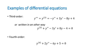
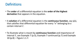
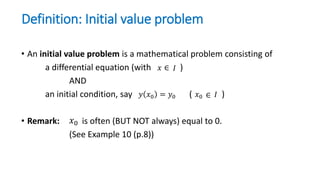
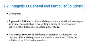
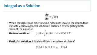
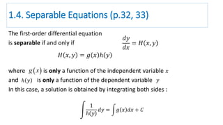
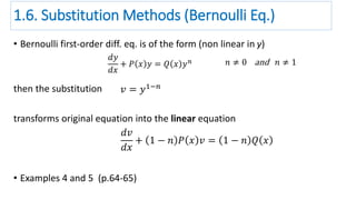
1. Differential Equations
&
Linear Algebra
MATH - 211

2. Book for the course
Differential Equations & Linear Algebra
Third Edition
by
C. Henry Edwards & David E. Penney
Pearson International Edition

3. Chapter 1.
First-Order Ordinary Differential Equations

4. 1.1. Differential Equations and Math Models
• Definitions:
• A differential equation is an equation relating an unknown function
and one or more of its derivatives.
• A first-order differential equation is an equation relating an unknown
function and its first derivative.
• Solution(s) to a given differential equation is (are) function(s) that
satisfy that differential equation.
• In case of ORDINARY diff. eqs., unknown function depends on only
ONE independent variable.
• In case of PARTIAL diff. eqs., unknown function depends on TWO or
MORE independent variables.

5. Examples of differential equations
• First-order:
• t: independent variable belonging to an interval
• y(t): dependent variable (function)
• x: independent variable belonging to an interval
• y(x): dependent variable (function)
𝑦′
=
𝑑𝑦
𝑑𝑥
= 𝑥 + sin 𝑦
𝑦′ =
𝑑𝑦
𝑑𝑡
= 3𝑡 + 4𝑦 − 17

6. Examples of differential equations
• Second-order:
𝑦′′ = −12𝑦′ + 3𝑦 − 5
𝑦′′
= 2𝑦′
+ 14
𝑦′′
= −𝑦 + 3

7. Examples of differential equations
• Third-order:
or written in an other way
• Fourth-order:
𝑦′′′ = 𝑦 3 = −𝑦′′ + 3𝑦′ − 8𝑦 + 4
𝑦 3
+ 𝑦′′
− 3𝑦′
+ 8𝑦 − 4 = 0
𝑦 4
+ 2𝑦′′
− 6𝑦 + 5 = 0

8. Examples of Mathematical Models
• Example 3 (p.2)
• Example 4 (p.2)
• Example 5 (p.3)
• Example 6 (p.3)

9. Definitions
• The order of a differential equation is the order of the highest
derivative that appears in the equation.
• A solution of a differential equation is the continuous function, say y(x),
that satisfies that differential equation for every “x” belonging to a
certain interval I .
• To illustrate what is meant by continuous function and importance of
interval I , see Example 7 (p.5), Example 7 continued (p.7) and Example
10 (p.8) – Figure 1.1.7.

10. Definition: Initial value problem
• An initial value problem is a mathematical problem consisting of
a differential equation (with )
AND
an initial condition, say ( )
• Remark: is often (BUT NOT always) equal to 0.
(See Example 10 (p.8))
𝑦 𝑥0 = 𝑦0
𝑥0
𝑥 ∈ 𝐼
𝑥0 ∈ 𝐼

11. Definition: Solution of an Initial value problem
• A solution of an initial value problem is the continuous function, say
y(x), that satisfies BOTH
the differential equation (for all )
AND
the initial condition, say ( )
For illustration, see Example 10 (p.8) and Figure 1.1.7.
𝑦 𝑥0 = 𝑦0
𝑥 ∈ 𝐼
𝑥0 ∈ 𝐼

12. Very Important Examples to Study:
Example 5 and Example 6 (p.3) **
** means “inspiration for Quiz/Exam questions”
Problems to Solve (p.8 and p.9) **
1 to 26 AND 32 to 36
** means “inspiration for Quiz/Exam questions”

13. 1.2. Integrals as General and Particular Solutions
• Definitions:
• A general solution of a differential equation is a function involving an
arbitrary constant (thus representing a family of functions) and
satisfying the differential equation under study.
• A particular solution of a differential equation is a function that
satisfies differential equation and an initial condition. This is the
solution of an initial value problem.

14. Integral as a Solution
• When the right-hand-side function f does not involve the dependent
variable y, then a general solution is obtained by integrating both
sides of the equation.
• General solution :
• Particular solution: initial condition is used to calculate C
𝑑𝑦
𝑑𝑥
= 𝑓 𝑥
𝑦 𝑥 = 𝑓 𝑥 𝑑𝑥 + 𝐶 = 𝐺 𝑥 + 𝐶
𝑦 𝑥0 = 𝑦0 ⇒ 𝐶 = 𝑦0 − 𝐺 𝑥0

15. Integral as a Solution
• Example 1 : p.11
• Velocity and Acceleration : p.12, 13
• Problems (p.17)** : 1 to 18
** means “inspiration for Quiz/Exam questions”

16. 1.4. Separable Equations (p.32, 33)
The first-order differential equation
is separable if and only if
where is only a function of the independent variable
and is only a function of the dependent variable
In this case, a solution is obtained by integrating both sides :
𝑑𝑦
𝑑𝑥
= 𝐻 𝑥, 𝑦
𝐻 𝑥, 𝑦 = 𝑔 𝑥 ℎ 𝑦
 g x 𝑥
ℎ 𝑦 𝑦
1
ℎ 𝑦
𝑑𝑦 = 𝑔 𝑥 𝑑𝑥 + 𝐶

17. 1.4. Separable Equations
• p. 32, p. 33; Example 1 (p.33) & Example 4 (p.36)
• p. 38, p. 39: Natural Growth Eq & Example 5 **
• p. 40, p.41: Cooling and Heating & Example 7 **
• Problems (p.43, p.44)**: 1 to 14; 19 to 27; 43, 44, 45, 46, 49
** means “inspiration for Quiz/Exam questions”

18. 1.5. Linear First-Order Equations (p.48-56)
Linear first-order differential equation is of the form
This equation is linear with respect to the dependent variable
The integrating factor is defined as
• A general solution is given by
𝑑𝑦
𝑑𝑥
+ 𝑃 𝑥 𝑦 = 𝑄 𝑥
𝑦
𝑃 𝑥 , 𝑄 𝑥 : 𝑐𝑜𝑛𝑡𝑖𝑛𝑢𝑜𝑢𝑠 𝑓𝑢𝑛𝑐𝑡𝑖𝑜𝑛𝑠
𝜌 𝑥 = exp 𝑃 𝑥 𝑑𝑥
𝑦 𝑥 =
1
𝜌 𝑥
𝐶 + 𝜌 𝑥 𝑄 𝑥 𝑑𝑥

19. Applications
• Examples: 1, 2, 3, 4 and 5
• Problems (p.56)**: 1 to 24
** means “inspiration for Quiz/Exam questions”

20. 1.6. Substitution Methods
• Many first-order differential equation are neither separable nor linear.
• Some creativity is needed to transform a “difficult” differential equation
into one that we already know how to solve (separable or linear).
• We need to substitute a part of the original equation by defining a new
dependent variable (v). The function that links the new variable “v” and
the original variable “y” must be invertible.
• This process will transform our original equation written in terms of “y”
into a new differential equation written in terms of a new variable “v”.

21. Substitution Methods
• We will solve the new (simpler) differential equation in “v”.
• In order to get the solution “y” for our original differential equation, we
will use the previously defined function linking the new variable “v” to
the original variable “y”.
• Example 1 (p.61)
• Solve by substituting
𝑑𝑦
𝑑𝑥
= 𝑒 𝑦 𝑣 = 𝑒 𝑦

22. 1.6. Substitution Methods (Homogeneous Eq.)
• If a first-order diff. eq. can be written in the homogeneous form
then the substitution
transforms initial equation into the separable equation
• Examples 2 and 3 (p.62-64)
𝑑𝑦
𝑑𝑥
= 𝐹
𝑦
𝑥
𝑣 =
𝑦
𝑥
, 𝑦 = 𝑣𝑥 ,
𝑑𝑦
𝑑𝑥
= 𝑣 + 𝑥
𝑑𝑣
𝑑𝑥
𝑥
𝑑𝑣
𝑑𝑥
= 𝐹 𝑣 − 𝑣

23. 1.6. Substitution Methods (Bernoulli Eq.)
• Bernoulli first-order diff. eq. is of the form (non linear in y)
then the substitution
transforms original equation into the linear equation
• Examples 4 and 5 (p.64-65)
𝑑𝑦
𝑑𝑥
+ 𝑃 𝑥 𝑦 = 𝑄 𝑥 𝑦 𝑛 𝑛 ≠ 0 and 𝑛 ≠ 1
𝑣 = 𝑦1−𝑛
𝑑𝑣
𝑑𝑥
+ 1 − 𝑛 𝑃 𝑥 𝑣 = 1 − 𝑛 𝑄 𝑥

24. Problems (p. 74)
• Problems **: 1 to 24; 26, 27
** means “inspiration for Quiz/Exam questions”
• Problem 28: suggestion – use substitution this should lead
you to Bernoulli Equation
𝑣 = 𝑒−𝑦

25. That is all
for
Chapter 1