This document provides an overview of linear systems and matrices. It discusses systems of linear equations, matrix notation, elementary row operations used to solve systems, echelon form, reduced row-echelon form, and examples of each. Key concepts covered include consistent and inconsistent systems, homogeneous systems, parametric solutions, and determining whether a matrix is in echelon/reduced echelon form. The document is organized into sections covering linear systems, matrices/Gaussian elimination, and reduced row-echelon matrices.

1. LINEAR SYSTEMS
AND
MATRICES

2. Systems of Linear Equations : Recall
Chapter 3
3.1 Introduction to Linear System : p.147 to p.154
p.155 Problems: 1 to 22
3.2 Matrices and Gaussian Elimination : p.156 to p.165
p.165 Problems: 1 to 27
3.3 Reduced Row-Echelon Matrices : p.167 to p.174
p. 174 Problems: 1 to 30

3. Systems of Linear Equations : Recall
System of m equations in n unknowns (x1,…., xn)
 A solution of the system must satisfy all equations at
the same time.
 Two linear systems are called equivalent if they have
the same solution set.
a11x1 a12 x2   a1nxn  b1
a21x1 a22 x2  a2n xn  b2
am1x1 am2 x2  amn xn  bm

4. Systems of Linear Equations : Recall
 A system of linear equations has
1. no solution (Example 2,4 p.148,150) , or
2. exactly one solution (Examples 1,3), or
3. infinitely many solutions (Example 5, p.151).
 A system of linear equations is said to be consistent
if it has either one solution or infinitely many
solutions.
 A system of linear equation is said to be
inconsistent if it has no solution.

5.  If , the system is called homogeneous.
 A homogeneous system always has at least one solution
which is
 A homogeneous system with more variables than
equations has infinitely many solutions.
b1 b2  bm  0
x1  x2   xn  0
Systems of Linear Equations : Recall
11 1 12 2 1
21 1 22 2 2
1 1 2 2
0
0
0
nn
nn
mn nm m
a x a x a x
a x a x a x
a x a x a x
   
   
   

6. Elementary Row Operations : Recall
The solution strategy for linear systems is to transform the
system through a series of equivalent systems until the
solution is obvious.
 Elementary row operations are:
1. (Replacement) Replace one row by the sum of
itself and a multiple of another row.
2. (Interchange) Interchange two rows.
3. (Scaling) Multiply all entries in a row by a nonzero
constant.
 Two matrices are called row equivalent if there is a
sequence of elementary row operations that transforms
one matrix into the other.

7.  If the augmented matrices of two linear systems are
row equivalent, then the two systems have the same
solution set.
 Elementary row operations guarantee that all
intermediate systems (matrices) obtained through this
process have the same set of solutions.
 Any combination of elementary row operations to a
linear system yields a new linear system that is
equivalent to the first.
Elementary Row Operations : Recall

8. Matrix Notation : Recall
Augmented matrix:
An m x n matrix is a rectangular array
of numbers with m rows and n columns.
(The number of rows always comes
first.)
If m=n then the matrix is called a square
matrix.
1
2
3
3x1 matrix3x1 matrix3x3 matrix
2 1 2 10
3 1 2 1
5 4 3 4
x
x
x
    
    
    
    
    

 
2x1  x2 2x3 10
3x1  x2 2x3  1
5x1 4x2  3x3  4
2 1 2 10
3 1 2 1
5 4 3 4
 
 
 
  

9.  System of m equations in n unknowns
 Notation: AX = b
 If b1 = b2 = … = bm = 0,
the system is homogenous
AX = 0
a11x1 a12 x2   a1nxn  b1
a21x1 a22 x2  a2n xn  b2
am1x1 am2 x2  amn xn  bm
Matrix Notation – General Case : Recall
11 12 1 1 1
21 22 2 2 2
1 2
n
n
mn n mm m
a a a x b
a a a x b
a a a x b
    
    
    
    
    
        

1
2
11 12 1
21 22 2
1 2 m
n
n
mnm m
b
b
b
a a a
a a a
a a a
 
 
 
 
 
  

10. infinitely many solutions with one
free variable
1 3
2 3
3
3 3
4
1 1 1
5 2 5 2
0 1
0 0 0
x x
x x
x
x x
x
        
          
         
       
       
      
2 1 0 4 7
0 1 2 0 5
0 0 0 3 0
0 0 0 0 0
 
 
 
 
 
 
3
is a free variablex
Solutions – Parametric Notation : Recall

11. infinitely many solutions with two
free variables
1 2 5
2 2
3 5 2 5
4 5
5 5
5 2 3 5 2 3
0 1 0
3 2 3 0 2
7 4 7 0 4
0 0 1
x x x
x x
x x x x
x x
x x
           
         
         
               
                  
                 
1 2 3 2 1 10
0 0 1 0 2 3
0 0 0 1 4 7
 
 
 
  
2 5
and are free variablesx x
Solutions – Parametric Notation : Recall

12. Echelon Form – Examples : Recall
7 1 4 3 0 2 0
0 0 3 8 4 3 2
0 0 0 2 2 1 2
0 0 0 0 0 1 3
0 0 0 0 0 0 0
 
  
 
 
 
  
0 3 1 4 3
0 0 1 6 5
0 0 0 0 1
 
 
 
  
2 3 1 4 0
0 5 1 0 5
0 0 3 0 1
 
 
 
  
1 2 3
0 6 1
 
 
 
1 0 3
0 1 1
 
  
9 0 0 2
0 0 3 6
0 0 0 7
0 0 0 0
 
 
 
 
 
 
2 1 0 1
0 3 9 4
0 0 2 0
0 0 0 4
 
 
 
 
 
 
1 4 3
0 0 2
 
 
 

13. Reduced Echelon Form – Examples : Recall
1 2 0 1 1
0 0 1 3 4
0 0 0 0 0
 
 
 
  
1 0 0 2
0 1 0 1
0 0 1 3
 
 
 
  
0 1 0 4 0
0 0 1 6 0
0 0 0 0 1
 
 
 
  
1 0 0 4 0
0 1 0 0 5
0 0 1 0 1
 
 
 
  
1 0 0 1
0 1 0 4
0 0 1 0
0 0 0 0
 
 
 
 
 
 
1 4 0
0 0 1
 
 
 
1 0 3
0 1 1
 
 
 
1 0 0 0
0 1 0 0
0 0 1 0
0 0 0 1
 
 
 
 
 
 1 0 0 4 3
0 1 0 2 5
0 0 1 1 1
 
 
 
  
1 0
0 1
 
 
 

14. Not Echelon Form – Examples : Recall
0 1 0 4 0
3 0 1 6 0
0 0 0 0 1
 
 
 
  
0 0 0 1 1
0 0 1 3 4
0 0 0 0 0
 
 
 
  
1 0 0 2
0 0 0 0
0 0 1 3
 
 
 
  
1 0 0 0
0 1 0 0
0 0 1 0
1 0 0 1
 
 
 
 
 
 
3 0 0 4 0
0 1 0 0 5
0 2 1 0 1
 
 
 
  
7 0 0 1
0 1 0 4
0 0 3 0
0 0 2 0
 
 
 
 
 
 
1 4 0
2 0 1
 
 
 
0 0
0 1
 
 
 
4 3 3
2 1 1
  
   
2 5 0 4 3
0 1 0 2 5
0 3 1 1 1
 
 
 
  

15. Matrix Operations
p.175 to p.185
3.4

16. Basic Operations on Matrices
a) Addition
b) Scalar multiplication
c) Matrix multiplication
3.4 Matrix Operations

17. Let A be a general m x n matrix
 i th row of A
 j th column of A
 Will sometimes write A = [ aij ]
 Will sometimes write ( A )ij for aij
ai1 ai2 ain  1i  m
1
2
1
j
j
mj
a
a
j n
a
 
 
 
 
 
 
  
 
3.4 Matrix Operations: General Notation

18.  If m  n then A is called a square matrix (same
number of equations and unknowns)
 For a square matrix, the elements
a11, a22, …, ann constitute the main diagonal of A
 Two matrices, A  [ aij ] and B  [ bij ], are equal
if they have the same dimensions and aij  bij for
1 ≤ i ≤ m, 1 ≤ j ≤ n
3.4 Matrix Operations: General Notation

19. Diagonal matrix is a square nxn matrix A  [ aij ]
where aij  0 for i ≠ j, i.e. the terms off the main
diagonal are all zero.
3 0 0 0
0 4 0 0
0 0 8 0
0 0 0 5
 
 
 
 
  
3.4 Matrix Operations: Diagonal Matrix
9 0 0
0 0 0
0 0 2
 
 
 
  
0 0 0
0 0 0
0 0 0
 
 
 
  
1 0 0
0 1 0
0 0 1
 
 
 
  
8 0
0 3
 
 
 
2 0
0 0
 
 
 0 0
0 1
 
 
 
0 0
0 0
 
 
 

20. Identity matrix is a square nxn matrix In  [ aij ]
where aii  1 and aij  0 for i ≠ j, i.e. the terms off
the main diagonal are all zero and the terms on the
main diagonal are all equal to 1.
4
1 0 0 0
0 1 0 0
0 0 1 0
0 0 0 1
 
 
 
 
 
 
I
3.4 Matrix Operations: Identity Matrix
3
1 0 0
0 1 0
0 0 1
 
 
 
  
I 2
1 0
0 1
 
  
 
I
 1
1I

21. Zero matrix is an mxn matrix 0mxn  [ aij ] where
aij  0 for all i and j, i.e. all terms are zero.
4
0 0 0 0
0 0 0 0
0 0 0 0
0 0 0 0
 
 
 
 
 
 
0
3.4 Matrix Operations: Zero Matrix
3
0 0 0
0 0 0
0 0 0
 
 
 
  
0 2x2
0 0
0 0
 
  
 
0
 1x1
00  1x2
0 00  1x3
0 0 00 3x1
0
0
0
 
 
 
  
0
2x4
0 0 0 0
0 0 0 0
 
  
 
0

22.  Adding matrices means adding corresponding
elements, e.g.
 Let A = [ aij ] and B = [ bij ] be two m x n matrices,
then C = A + B is a m x n matrix C = [ cij ] such that
cij = aij + bij for all i, j
 Note: sizes of matrices must be the same
1 2 3 3 2 1 4 4 4
4 5 6 6 5 4 10 10 10
     
     
     
 
1 2 1 2 3
3 4 4 5 6
   
   
   
 undefined
3.4 Matrix Operations: Matrix Addition

23.  Scalar multiplication means multiplying each element
of a matrix by the same scalar, e.g.
 Let A = [ aij ] and r  R
Then C = r A, where
C = [ cij ] is defined as cij = r aij  i, j
1 2 2 4
2
3 4 6 8
   
   
   

3.4 Matrix Operations: Scalar Multiplication
4 1 3 8 2 6
2
2 5 0 4 10 0
   
   
   
  
 
 

24. ( 1)
1 2 3 1 2 3 1 2 3
4 5 6 4 5 6 4 5 6
     
       
     
  

  
undefined
3.4 Matrix Operations: Remarks
2
4 2 4 1
1
 
 
    
 
 
2
4 2 4 1
1
 
 
    
 
 
2
5
4
9
1
 
  
   
  
 
undefined
 3 6
2
4
1
 
 
  
 
 
undefined
4
3 2 6
3
2 5
4 9
1 0
     
            
        
     1 5 3 2 1 4 1 4 1   

25. See p. 181 Examples 5 & 6
3.4 Matrix Operations: Matrix Multiplication

26. We want to express
So, need to have matrix multiplication to work like
e.g.
11 12 111 1 12 2 1 1
21 22 221 1 22 2 2 2
as
a a xa x a x b b
a a xa x a x b b
    
    
          
 

 
11 12 1 11 1 12 2
21 22 2 21 1 22 2
a a x a x a x
a a x a x a x
    
    
        



1 2 5 6 1 5 2 7 1 6 2 8 19 22
3 4 7 8 3 5 4 7 3 6 4 8 43 50
      
      
      
     
 
     
3.4 Matrix Operations: Matrix Multiplication

27. If A is m x n and X is n x 1, can also express AX as
We call this a linear combination of the columns of A.
The coefficients are the elements of X.
11 12 1
21 22 2
1 2
1 2
n
n
n
mnm m
a a a
a a a
x x x
a a a
     
     
     
     
     
         
   AX
3.4 Matrix Operations: Matrix Multiplication

28. What about
 The basic idea is to multiply each column of B by A
11 12 111 12 1
21 22 2 21 22 2
1 2 1 2
pn
n p
mnm m npn n
b b ba a a
a a a b b b
a a a b b b
  
  
  
  
  
      
A B
111 12
221 22
1 2
p
p
n n np
bb b
bb b
b b b
                                     
AB A A A
3.4 Matrix Operations: Matrix Multiplication

29. Examine the first column of product
1 1
1
11
2 121
1
1
1
1
n
k k
k
n
k k
k
n n
mk k
k
a b
b
a bb
b
a b



 
 
  
  
  
  
  
     
 
  




A
1st row A x 1st column B
2nd row A x 1st column B
mth row A x 1st column B
3.4 Matrix Operations: Matrix Multiplication

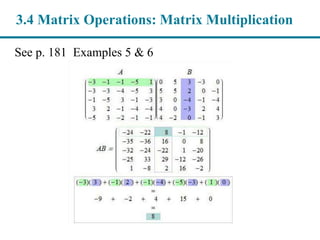
30. Defn. Let A = [ aij ] be an m x n matrix and let
B = [ bij ] be an q x p matrix.
 The product of A and B is defined if and only if n=q
Then, AB = C = [ cij ], is the m x p matrix defined by
 The product of B and A is defined if and only if m=p
Then, BA = D = [ dij ], is the q x n matrix defined by
1 1 2 2
1
for 1,2, , 1,2, ,
n
ij in nji j i jik kj
k
c a b a b a b a b i m j p

      
3.4 Matrix Operations: Matrix Multiplication
1 1 2 2
1
for 1,2, , 1,2, ,
m
ij in nji j i jik kj
k
d b a b a b a b a i q j n

      

31. 3.4 Matrix Addition: Properties
Let A, B and C be m x n matrices
1) A + B is an m x n matrix
2) A + (B + C) = (A + B) + C
3) There is a unique m x n matrix m0n such that
A + m0n = m0n + A = A for every matrix A
4) For every m x n matrix A, there is a unique m x n
matrix D such that A + D = D + A = m0n
5) A + B = B + A

32. 3.4 Matrix Multiplication: Properties
 If A, B and C are matrices of the appropriate sizes, then
A(BC)  (AB)C
 If A, B and C are matrices of the appropriate sizes, then
(A + B)C  AC + BC
 If A, B and C are matrices of the appropriate sizes, then
C(A + B)  CA + CB
 Let A be any mxn matrix,
then A In  A and Im A  A
 Let A be any mxn matrix,
then A 0nxp  0mxp and 0qxm A  0qxn

33. Comments on Matrix Multiplication
 AB need not equal BA
 Let
So, we can have AB  0, but A ≠ 0 and B ≠ 0
 BA = ?

1 2 4 6 0 0
2 4 2 3 0 0
     
     
     

   

A B AB
1 2 2 1 2 7
Let , ,
2 4 3 2 5 1
8 5
then but , i.e. can't cancel
16 10
     
     
     
 
 
 

  

  
A B C
AB AC B C
3.4 Matrix Multiplication: Properties

34. Example 8 (p.185) 51 3 4
14 1 2 7 3 2 1
43 1 1 5 2 2 3
32 1 3
25 10
and
18 5
   
   
     
          
      
 
 
 

  
  
 

  

A B C
AB AC B C
3.4 Matrix Multiplication: Properties
2 1
4 1 2 7 1 2 0 0
3 1 1 5 0 1 0 0
1 0
and , are non zero matrices
 
 
    
        
  

 
   

A D AD
A D

35. AB BA
1 2 1 2 1 1
0 2 1 1 1 0
2 1 1 2 1 1
   
   
   
   
   
 
   A B
3.4 Matrix Multiplication: Properties
2 2 0 0 3 0
0 1 1 1 4 2
7 0 1 4 5 4
   
   
   
   
   

    
 
AB BA
AB BA

36. If r and s are real numbers and A and B are matrices,
then
 r ( sA )  ( rs ) A
 ( r + s ) A  rA + sA
 r ( A + B )  rA + rB
 A ( rB )  r ( AB )  ( rA ) B
3.4 Scalar Multiplication: Properties

37. Let A  [ aij ] be an m x n matrix.
The transpose of A, AT  [ aij
T ], is the n x m matrix
defined by aij
T  aji
T1 2 1 3
3 4 2 4
   
   
   
 A A
3.4 Matrix Operations: Matrix Transpose
T 3
3 5
5
 
    
 
  

B B
T
1 2
1 3 4
3 5
2 5 6
4 6
 
   
   
   
 
 C C

38. If r is a scalar and A and B are matrices, then
 ( AT )T  A
 ( A + B )T  AT + BT when AT  A
 ( AB )T  BTAT A is called symmetric
 ( rA )T  rAT
Find transpose matrix for:
3.4 Matrix Transpose: Properties
2 3
1 4
5 6
 
 
 
 
 
3 5 2
5 4 1
2 1 7
 
 
 
 
 


1 3 4 
 

39.  The following laws of exponents hold for nonnegative
integers p and q and any n x n matrix A
1 ) Ap Aq  Ap + q
2 ) ( Ap ) q  Apq
 Caution. Without additional assumptions on A and B,
cannot do the following
1 ) define Ap for negative integers p
2 ) assert that ( AB ) p  Ap B p
3.4 Matrix Powers: Properties

40.  An n x n matrix A  [ aij ] is called upper triangular
if and only if aij  0 for i > j
 An n x n matrix A  [ aij ] is called lower triangular
if and only if aij  0 for i < j
 Note:
 A diagonal matrix is both upper and lower triangular
 The n x n zero matrix is both upper and lower triangular
3.4 Special Matrices: Triangular Matrices

41.  Defn - A matrix A is called symmetric if AT A
 Defn - A matrix A is called skew-symmetric if AT A
 Comment - If A is skew-symmetric, then the diagonal
elements of A are zero
 Comment - Any square matrix A can be written as the
sum of a symmetric matrix and a skew-symmetric matrix
   T T
symmetric skew-symmetric
1 1
2 2
   A A A A A
3.4 Special Matrices: Symmetric Matrices

42. Symmetry
 For any matrix A, matrices AAT and AT A
are symmetric.
 If matrix A is square, then A+ AT is symmetric.
3.4 Special Matrices: Symmetric Matrices

43. Problems 3.4
p. 186
Problems : 1 to 27

44. Inverse of Matrices
p.188 to p.198
Only some (rare) Matrices have the Inverse
3.5

45. Nonsingular Matrices
 Defn - An n x n matrix A is called nonsingular or
invertible if there exists an n x n matrix B such that
AB  BA  In
 Comments
 If B exists, then B is called the inverse of A.
 Then, A is also the inverse of B.
 If B does not exist, then A is called singular or
noninvertible.
 At this point, the only available tool for showing that
A is nonsingular is to show that B exists
3.5 Inverse of Matrices : Definition
3 5 2 5
1 2 1 3
   
      
 A B

46. Nonsingular Matrices
 Theorem - If the inverse of a matrix exists, then that
inverse is unique.
 Proof - Let A be a nonsingular n x n matrix and let B and
C be inverses of A. Then AB  BA  In and
AC  CA  In B  B In  B( AC ) ( BA )C  In C  C
so the inverse is unique.
 Notation - If A is a nonsingular matrix, the inverse of A is
denoted by A1
 Comment - For nonsingular matrices, A, can define A
raised to a negative power as Ak  ( A1 ) k k > 0
3.5 Inverse of Matrices : Properties

47. Nonsingular Matrices
 Theorem - If A and B are both nonsingular matrices, then
the product AB is nonsingular and ( AB ) 1  B1A1
 Proof - Consider the following products
AB ( B1A1 )  AB B1A1  A In A1  AA1  In
and
( B1A1 ) AB  B1A1AB B1In B B1B In
Since we have found a matrix C such that C ( AB )  ( AB )
C In , AB is nonsingular and its inverse is C  B1A1
3.5 Inverse of Matrices : Properties

48. Nonsingular Matrices
 Theorem - If A1, A2, …, Ar are nonsingular matrices,
then A1 A2 • • • Ar is nonsingular and
 Theorem - If A is a nonsingular matrix, then A1 is
nonsingular and (A1)1  A
Proof: Since A1A  AA1 In , then A1 is nonsingular
and its inverse is A. So (A1)1  A.
A1A2 Ar 
1
 Ar
1
Ar1
1
A2
1
A1
1
3.5 Inverse of Matrices : Properties

49. Nonsingular Matrices
 Comment: We have observed earlier that AB  AC does
not necessarily imply that B  C. However, if A is an n x n
nonsingular matrix and AB  AC, then B  C.
A1 ( AB )  A1 ( AC )  ( A1A ) B  ( A1A ) C  B  C
 Comment: We have observed earlier that AB  n0n does not
imply that A  n0n or B  n0n. However, if A is an n x n
nonsingular matrix and AB  n0n , then B  n0n .
A1 ( AB )  A1
n0n  ( A1A ) B  n0n  B  n0n
3.5 Inverse of Matrices : Properties

50. Nonsingular Matrices
 Theorem - If A is a nonsingular matrix, then AT is
nonsingular and ( AT ) 1  ( A1 ) T
 Proof - By an earlier theorem, ( AB )T  BTAT for
any two matrices A and B. Since A is nonsingular,
A1 A  A A1 In . Applying the relationship on
transposes gives
In In
T ( A1 A )T  AT ( A1 )T
In In
T ( AA1 )T  ( A1 )T AT
Since AT ( A1 )T In and ( A1 )T AT In , AT is
nonsingular and its inverse is ( A1 )T , i.e.
( AT ) 1  ( A1 ) T
3.5 Inverse of Matrices : Properties

51. Linear Systems and Inverses
 A system of n linear equations in n unknowns may be
written as AX = b, where A is n x n matrix. If A is
nonsingular, then A1 exists and the system may be
solved by multiplying both sides by A1
A1( AX ) = A1b  ( A1A )X = A1b  X = A1b
 If A is an invertible matrix, then AX = b has a unique
solution for any b.
3.5 Inverse of Matrices : Properties

52. Linear Systems and Inverses
 Comment - Although X = A1B gives a simple
expression for the solution, its primary usage is for
proofs and derivations
 At this point we have no practical tool for computing
A1
 Even with a tool for computing A1, this method of
solution is usually numerically inefficient. The only
exception is if A has a special structure that lets A1
have a simple relationship to A
3.5 Inverse of Matrices : Properties

53. Linear Systems and Inverses
 AX = b
If then
 For k non zero scalar and A an invertible matrix
3.5 Inverse of Matrices : Properties
a b
c d
 
 
 
A
0ad bc 
1 1 d b
ad bc c a
  
   
A
 
1 11
k
k
 
A A

54. 3.5 Inverse of Matrices : Simple Cases
1 1
n n n
 
 A I A I I
1
1
0 0 0 0
10 0 0 0 0 0 0 0
0 0 0 0
1
, , , , , 00 0 0 0 0 0 0 0
0 0 0 0
1
0 0 0 00 0 0 0
1
0 0 0 0
a
a
bb
a b c d ec
c
d
e d
e

 
 
 
   
   
   
   
   
   
    
 
 
  
 D D