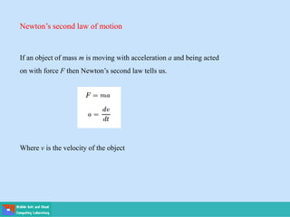
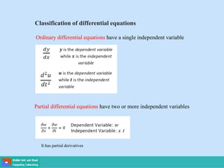
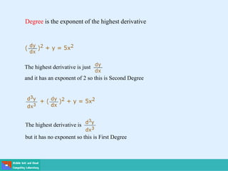
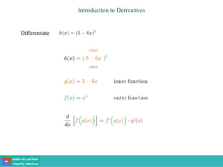
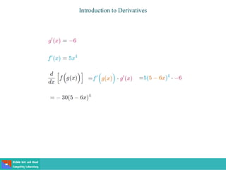
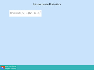
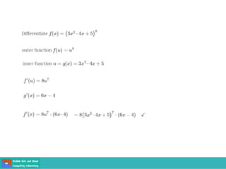
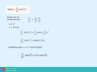
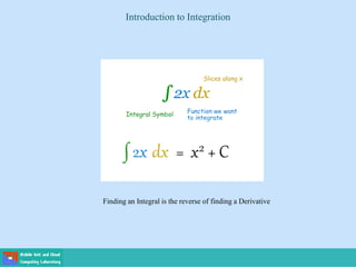
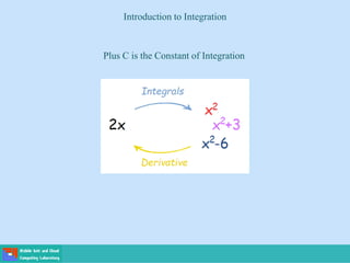
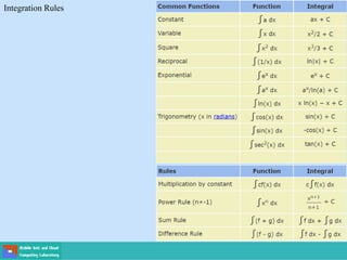
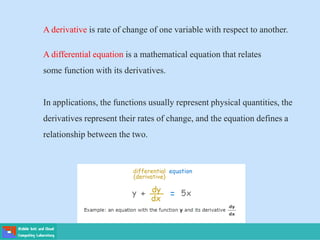
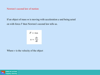
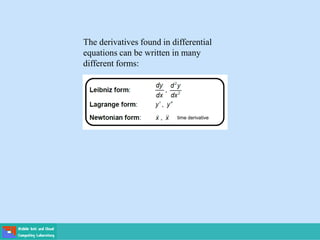
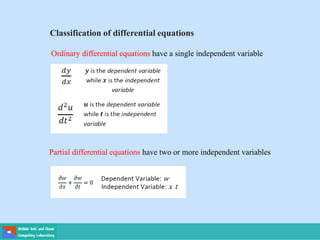
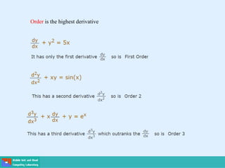
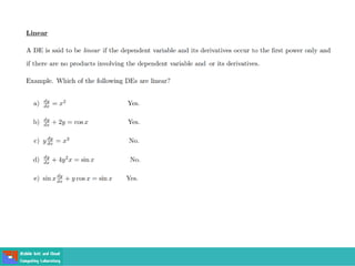
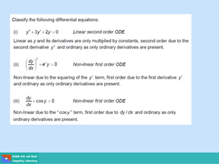
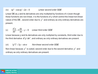
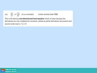
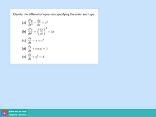
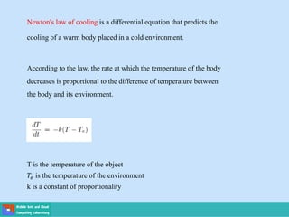
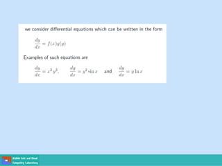
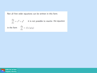
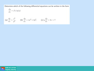
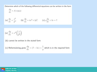
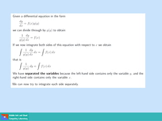
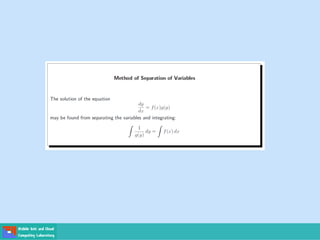
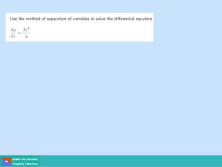
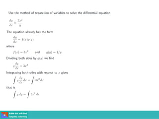
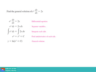
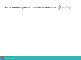
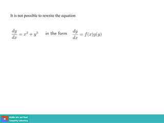
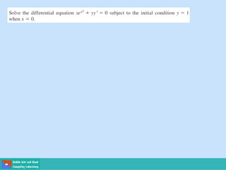
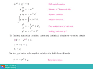
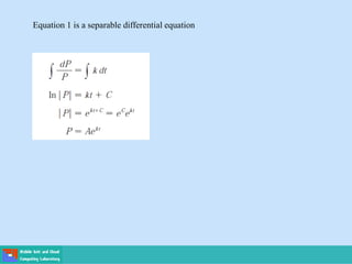
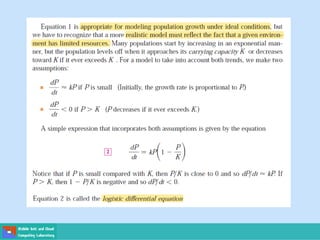
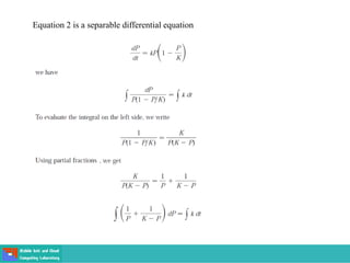
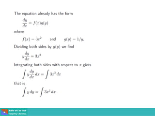
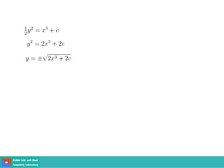
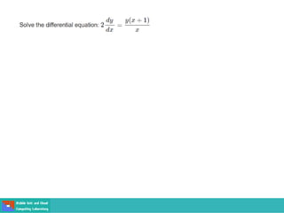
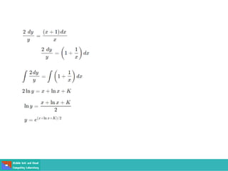
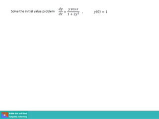
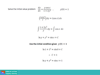
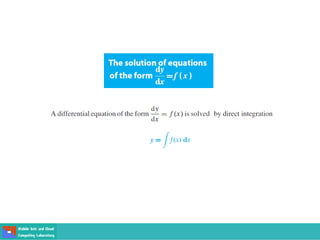
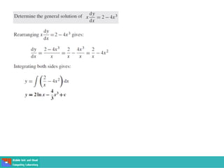
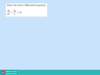
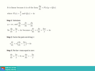
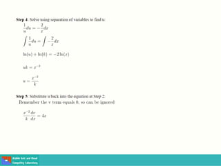
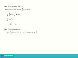
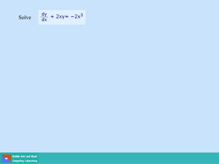
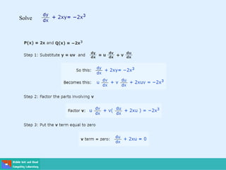
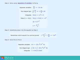
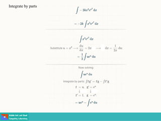
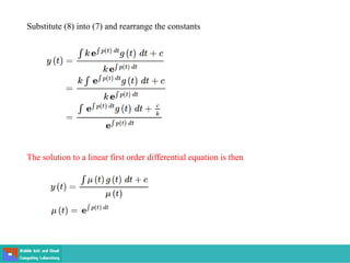
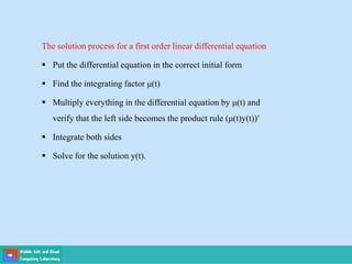
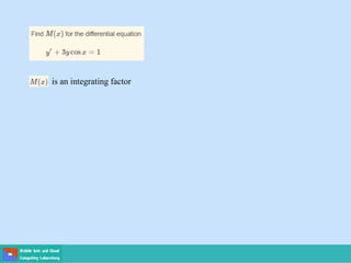
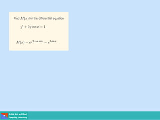
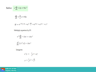
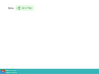
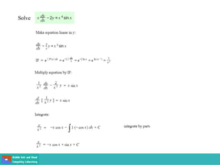
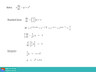
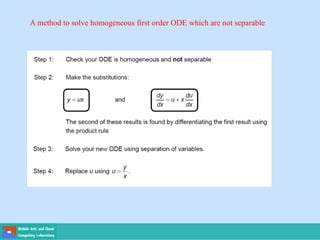
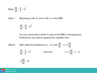
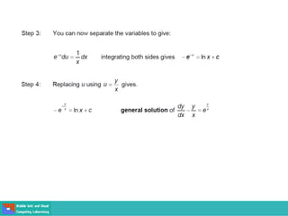
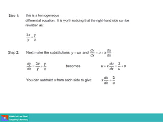
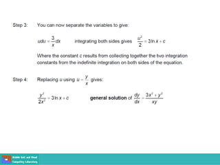
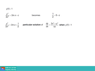
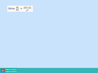
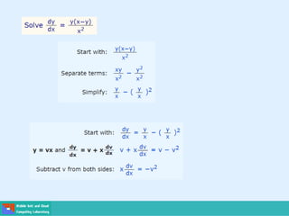
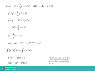
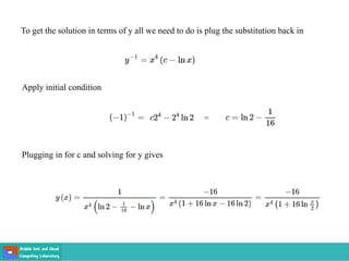
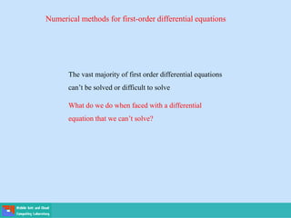
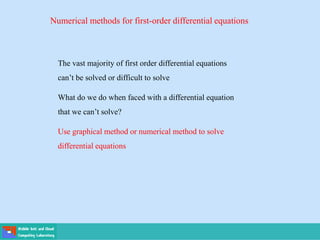
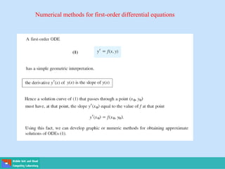
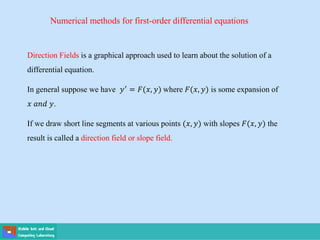
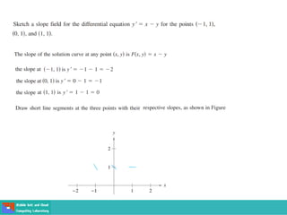
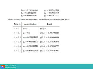
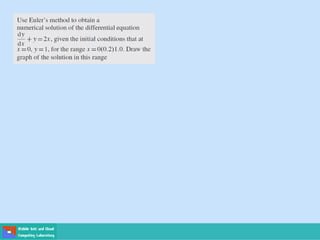
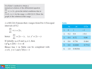
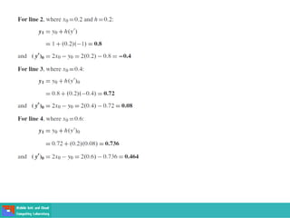
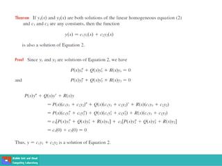
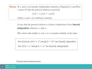
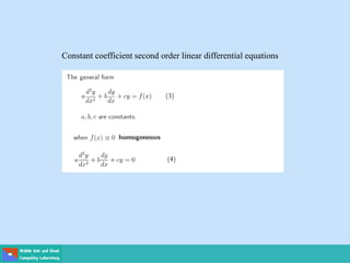
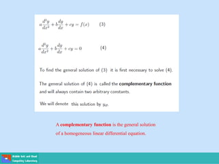
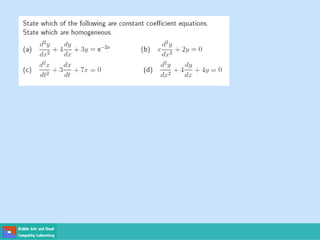
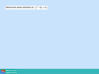
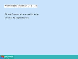
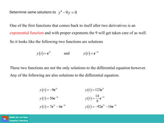
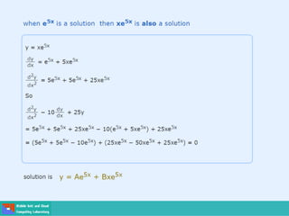
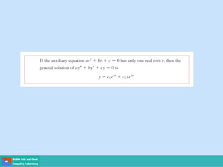
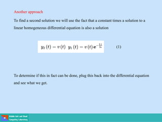
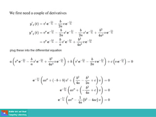
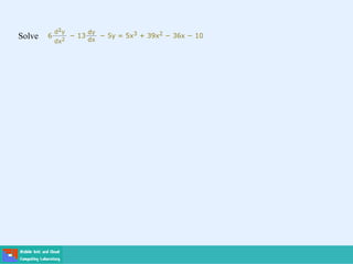
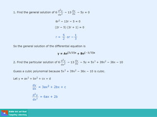
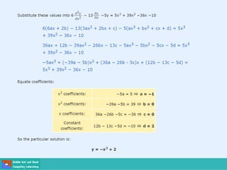
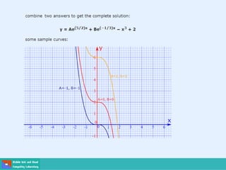
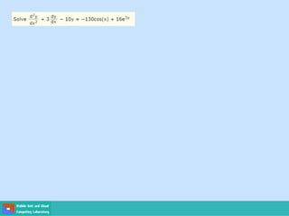
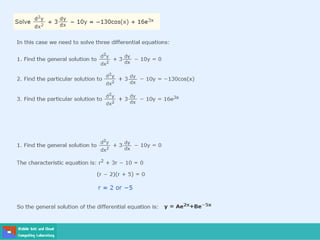
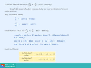
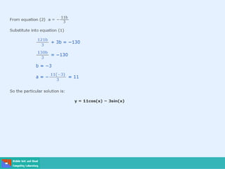
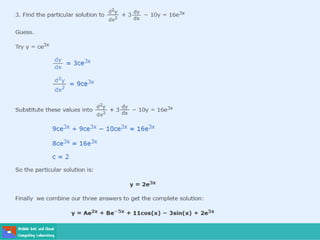
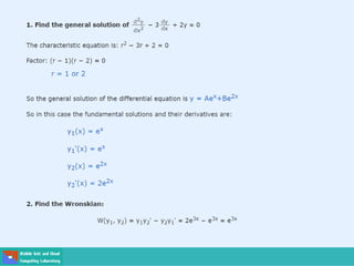
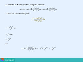
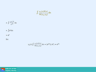
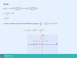
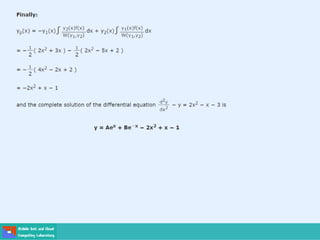
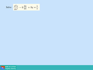
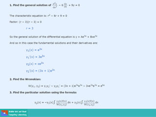
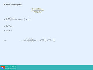
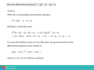
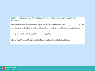
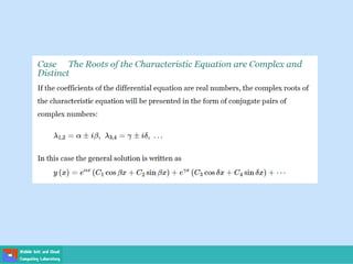
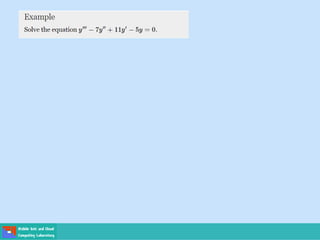
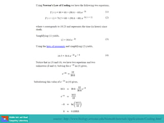
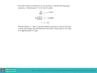
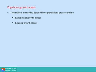
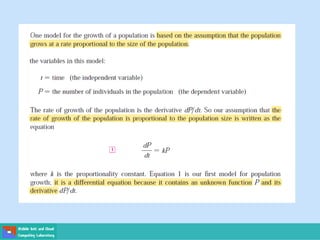
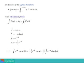
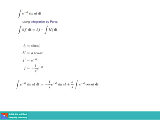
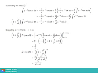
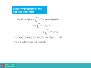
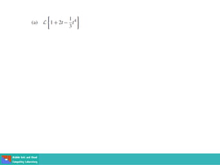
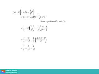
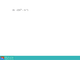
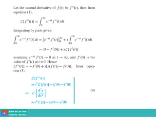
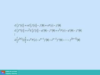
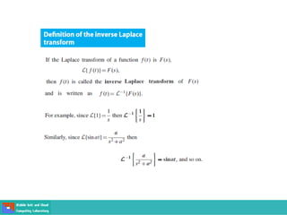
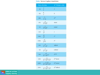
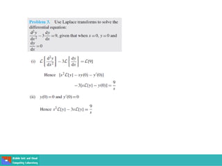
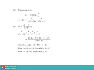
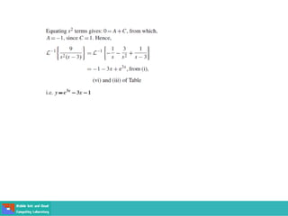
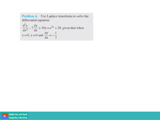
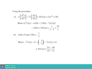
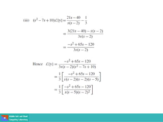
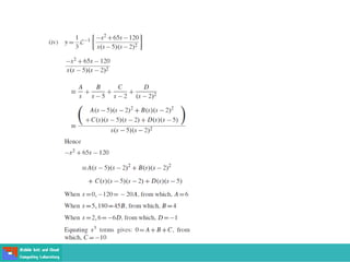
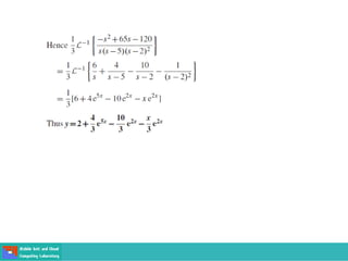
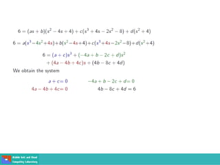
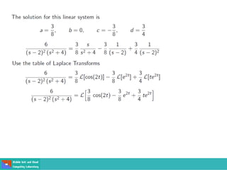
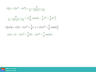
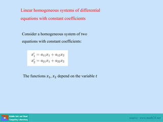
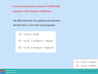
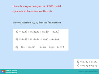
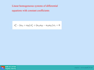
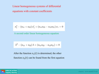
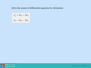
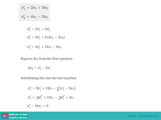
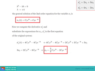
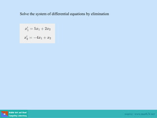
Introduction to Differential Equations

Engineering Mathematics I
Sayed Chhattan Shah
Associate Professor of Computer Science
Mobile Grid and Cloud Computing Lab
Department of Information Communication Engineering
Hankuk University of Foreign Studies Korea
www.mgclab.com

Acknowledgements
 The material in these slides is taken from different sources
including:
o Advanced Engineering Mathematics by Erwin Kreyszig
o Understanding Engineering Mathematics by John Bird
o Calculus by James Stewart
o Differential Equations by Learning Enhancement Team at University of East Anglia
o Differential Equations accessible at
http://epsassets.manchester.ac.uk/medialand/maths/helm/
o Differential Equations accessible at http://tutorial.math.lamar.edu/Classes/DE/DE.aspx
o Calculus accessible at https://www.mathsisfun.com/calculus/

A derivative is rate of change of one variable with respect to another.
A differential equation is a mathematical equation that relates
some function with its derivatives.
In applications, the functions usually represent physical quantities, the
derivatives represent their rates of change, and the equation defines a
relationship between the two.

Newton’s second law of motion
If an object of mass m is moving with acceleration a and being acted
on with force F then Newton’s second law tells us.
Where v is the velocity of the object

Newton's law of cooling is a differential equation that predicts the
cooling of a warm body placed in a cold environment.
According to the law, the rate at which the temperature of the body
decreases is proportional to the difference of temperature between
the body and its environment.
T is the temperature of the object
𝑇𝑒 is the temperature of the environment
k is a constant of proportionality

The derivatives found in differential
equations can be written in many
different forms:
time derivative

Classification of differential equations
Ordinary differential equations have a single independent variable
Partial differential equations have two or more independent variables
It has partial derivatives

Order is the highest derivative

Degree is the exponent of the highest derivative
The highest derivative is just
and it has an exponent of 2 so this is Second Degree
The highest derivative is
but it has no exponent so this is First Degree

 Multivariable functions
o A function is called multivariable if its input is made up of multiple numbers.
o If the output of a function consists of multiple numbers, it is called
multivariable and also vector-valued function

 Examples of multivariable functions
o From location to temperature

 In single variable calculus
At a given value of a
f′(a) measures the instantaneous rate of change of function f
Introduction to Derivatives

 Alternate notation

 Differentiation Formulas

The chain rule is a formula to compute the derivative of a composite function
The rule says that the derivative of the composite function is the inner
function g within the derivative of the outer function f’ multiplied by the
derivative of the inner function g’

Differentiate

Another way of
writing chain rule

Introduction to Integration
Finding an Integral is the reverse of finding a Derivative

Plus C is the Constant of Integration

Integration by Substitution is a method to find an integral
but only when it can be set up in a special way.

Integration by Parts is a special method of integration that is often useful
when two functions are multiplied together
Reverse of the product rule of differentiation

Introduction to partial derivatives

It says as only the radius changes the volume changes by

It says as only the height changes the volume changes by

Find all of the partial derivatives for the following function.
Introduction to partial derivatives

Find all of the partial derivatives for the following function.

Classification of differential equations
Ordinary differential equations have a single independent variable
Partial differential equations have two or more independent variables

Solving a differential equation
Solving a differential equation finds functions which
satisfy the conditions described by the DE.
For example the linear second order ODE:
Solving this ODE means the same as finding any
functions which satisfy this relationship.

Solving a differential equation: general solution
A solution to a differential equation
which contains one or more arbitrary constants
of integration is called the general solution of
the differential equation.

Particular solutions and initial conditions
A particular solution of a differential equation is any solution that is
obtained by assigning specific values to the arbitrary constants in
the general solution.

Geometrically, the general solution of a differential equation
represents a family of curves known as solution curves.
For instance, the general solution of the differential equation
Figure shows several solution curves corresponding to
different values of C

Particular solutions of a differential equation are obtained
from initial conditions placed on the unknown function and
its derivatives.
Suppose you want to find the particular solution whose
graph passes through the point (1, 3)
This initial condition can be written as
Substituting these values into the general solution produces
which implies that
So, the particular solution is

Applications Differential Equations

Acceleration is the rate of change of velocity with respect to time
The acceleration a equals the second derivative of the position x
with respect to t

Population growth models
 Two models are used to describe how populations grow over time.
 Exponential growth model
 Logistic growth model

Separation of Variables
Separation of variables is a technique commonly used to solve first
order ordinary differential equations.
It is so-called because we rearrange the equation to be solved such
that all terms involving the dependent variable appear on one side
of the equation, and all terms involving the independent variable
appear on the other.

Use the method of separation of variables to solve the equation

It is not possible to rewrite the equation

Equation 1 is a separable differential equation

Equation 2 is a separable differential equation

Solve the equation
The left side is a simple logarithm, the right side can be
integrated using substitution:

First order linear differential equations
A first-order linear differential equation is an equation of the form
where P and Q are functions of x
An equation that is written in this form is said to be in standard form.

A step-by-step method 1
1. Substitute y = uv and
2. Factor the parts involving v
3. Put the v term equal to zero
4. Solve using separation of variables to find u
5. Substitute u back into the equation we got at step 2
6. Solve that to find v
7. Substitute u and v into y = uv to get solution

Solving differential equations with integrating factors

To help you understand how multiplying by an integrating factor works,
equation is set up to practically solve itself
Multiply every term by
The two terms on the left side of the equation just happen to be the result of the
application of the Product Rule to the expression

To undo the derivative on the left side, integrate both sides, and then solve for y:
To check this solution, plug this value of y back into the original equation:

The previous example works because we found a way to multiply the entire equation
by a factor that made the left side of the equation look like a derivative resulting from
the Product Rule.

In the previous example
2 ln x = ln x2

In order to solve a linear first order differential equation we MUST start with the
differential equation in the form shown below.
Assume that there is some magical function μ(t) called an integrating factor
Now that we have assumed the existence of μ(t) multiply everything in (1) by μ(t)
Assume that whatever μ(t) is, it will satisfy the following

Again do not worry about how we can find a μ(t) that will satisfy (3)
So substituting (3) we now arrive at
At this point we need to recognize that the left side of (4) is nothing more
than the following product rule.

So we can replace the left side of (4) with this product rule.
Integrate both sides of (5) to get.

The final step is then some algebra to solve for the solution, y(t)

So, now that we’ve got a general solution to (1) we need to go back and
determine just what this magical function μ(t) is
Start with (3)
Exponentiate both sides to get μ(t) out of the natural logarithm.
Integrating factor R
Separation of variables technique
review

Substitute (8) into (7) and rearrange the constants
The solution to a linear first order differential equation is then

The solution process for a first order linear differential equation
 Put the differential equation in the correct initial form
 Find the integrating factor μ(t)
 Multiply everything in the differential equation by μ(t) and
verify that the left side becomes the product rule (μ(t)y(t))′
 Integrate both sides
 Solve for the solution y(t).

Homogeneous ODE
A first order ODE is called homogeneous if the DE remains
unchanged if you can replace y with ty and x with tx

Which of these first order ordinary differential equations are homogeneous?

A method to solve homogeneous first order ODE which are not separable

Bernoulli Differential Equations
When n = 0 the equation can be solved as a First Order Linear Differential Equation
When n = 1 the equation can be solved using Separation of Variables
For other values of n we can solve it by substituting
(1)

Bernoulli Differential Equations
To reduce the equation to a linear equation, use substitution
(2)

Method of solution
Solve the first order differential equation using the technique of an integrating factor

The absolute value bars on the x
in the logarithm are dropped
because of the assumption that
x > 0

To get the solution in terms of y all we need to do is plug the substitution back in
Apply initial condition
Plugging in for c and solving for y gives

Numerical methods for first-order differential equations
The vast majority of first order differential equations
can’t be solved or difficult to solve
What do we do when faced with a differential
equation that we can’t solve?

The vast majority of first order differential equations
can’t be solved or difficult to solve
What do we do when faced with a differential equation
that we can’t solve?
Use graphical method or numerical method to solve
differential equations

Direction Fields is a graphical approach used to learn about the solution of a
differential equation.
In general suppose we have 𝑦′ = 𝐹(𝑥, 𝑦) where 𝐹(𝑥, 𝑦) is some expansion of
𝑥 𝑎𝑛𝑑 𝑦.
If we draw short line segments at various points (𝑥, 𝑦) with slopes 𝐹(𝑥, 𝑦) the
result is called a direction field or slope field.

Euler’s method is a numerical approach to approximating the particular solution
of the differential equation
that passes through the point
From the given information, we know that the graph of the solution passes
through the point and has a slope of at this point.
This gives us a starting point for approximating the solution

From this starting point, we can proceed in the direction indicated by the slope.
Using a small step h, move along the tangent line until we arrive at the point
where

If you think of as a new starting point, you can repeat the process to
obtain a second point

Second Order Differential Equations

Proved in more advanced courses

Constant coefficient second order linear differential equations

A complementary function is the general solution
of a homogeneous linear differential equation.

We need functions whose second derivative
is 9 times the original function.

One of the first functions that comes back to itself after two derivatives is an
exponential function and with proper exponents the 9 will get taken care of as well.
So it looks like the following two functions are solutions
These two functions are not the only solutions to the differential equation however.
Any of the following are also solutions to the differential equation.

 How do we to find solutions to a linear constant
coefficient, second order homogeneous
differential equation?
 First write down the characteristic equation for
the differential equation.
 This will be a quadratic equation and so we
should expect two roots and .
 Once we have these two roots we have two
solutions to the differential equation.

Solving the characteristic or auxiliary equation
gives the values of r which we need to find the
solutions.
The nature of the roots will depend upon the
values of a, b and c.

Another approach
To find a second solution we will use the fact that a constant times a solution to a
linear homogeneous differential equation is also a solution
To determine if this in fact can be done, plug this back into the differential equation
and see what we get.
(1)

We first need a couple of derivatives

Because we are working with a double root we know that that the second term will
be zero. Also exponentials are never zero. Therefore (1) will be a solution to the
differential equation provided v(t) is a function that satisfies the following
differential equation.
We can drop the a because we know that it can’t be zero
The two solutions are

Euler's Formula for Complex Numbers
A Taylor Series is an expansion of some function into an infinite
sum of terms where each term has a larger exponent

The particular integral
There are two main methods to solve equation
 Undetermined Coefficients works when f(𝑥) is a polynomial,
exponential, sine, cosine or a linear combination of those.
 Variation of Parameters which is a little messier but works on a wider
range of functions.

A particular integral is any
solution of a differential equation.

Finding a particular integral
Method involves trial and error and educated guesswork.
We try solutions which are of the same general form as f(x) on
right hand side.

We shall attempt to find a solution of the inhomogeneous problem by trying a function of the same
form as that on the right-hand side of the ODE.

Table provides a summary of the trial solutions which
should be tried for various forms of the right-hand side.

Finding the general solution of a second order linear inhomogeneous ODE
Particular solutions of the non-homogeneous equation plus
the general solution of the homogeneous equation

Check if the answer is correct:

Initial-Value and Boundary-Value Problems
An initial-value problem for the second-order equation consists of
finding a solution y of the differential equation that also satisfies initial
conditions of the form
𝑦 𝑥0 = 𝑦0 𝑦′
𝑥0 = 𝑦1
where 𝑦0 and 𝑦1 are given constants

Initial-Value and Boundary-Value Problems
A boundary-value problem for equation consists of finding a solution y of
the differential equation that also satisfies boundary conditions of the form
𝑦 𝑥0 = 𝑦0 𝑦 𝑥1 = 𝑦1

The Fundamental Solutions of The Equation
Previously we discussed how to find the general solution of
following differential equation
In all three cases above y is made of two parts: 𝑦1 and 𝑦2
y1 and y2 are known as the fundamental solutions of the equation and y1 and
y2 are said to be linearly independent because neither function is a constant
multiple of the other.

Linear Independence and the Wronskian
Two functions are linearly independent on some open interval if neither
function is a scalar multiple of the other

If the Wronskian does not equal 0 the two functions are independent

The Wronskian
When y1 and y2 are the two fundamental solutions of the homogeneous equation
then the Wronskian W(y1, y2) is the determinant of the matrix
so W 𝑦1, 𝑦2 = 𝑦1𝑦2′ − 𝑦2𝑦1′
Since y1 and y2 are linearly independent, the value of the Wronskian cannot equal zero.
𝑦1 𝑦2
𝑦1′ 𝑦2′

Using the Wronskian we can find the particular solution of DE
using formula

Introduction to Higher Order Linear
Homogeneous Differential Equations with Constant Coefficients

Applications of Differential Equations

Newton's law of cooling can be used to model the growth or decay
of the temperature of an object over time.
According to the law, the rate at which the temperature of the body
decreases is proportional to the difference of temperature between
the body and its environment.
T is the temperature of the object
𝑇𝑒 is the temperature of the environment
k is a constant of proportionality

Newton's law of cooling
T (t) is the temperature of the object at time t
Te is the constant temperature of the environment
T0 is the initial temperature of the object
k is a constant that depends on the material properties of the object.

source: http://www.biology.arizona.edu/biomath/tutorials/Applications/Cooling.html
A detective is called to the scene of a crime where a dead body has just been
found. She arrives on the scene at 10:23 pm and begins her investigation.
Immediately the temperature of the body is taken and is found to be 80o F. The
detective checks the programmable thermostat and finds that the room has been
kept at a constant 68o F for the past 3 days.
After evidence from the crime scene is collected, the temperature of the body is
taken once more and found to be 78.5o F. This last temperature reading was taken
exactly one hour after the first one. The next day the detective is asked by another
investigator, what time did our victim die? Assuming that the victim’s body
temperature was normal (98.6o F) prior to death, what is her answer to this
question?

We would like to know the time at which a person died.
In particular, we know the investigator arrived on the scene at 10:23 pm, which
we will call τ hours after death.
10:23 (τ hours after death) the temperature of the body was found to be 80o F.
One hour later, τ + 1 hours after death, the body was found to be 78.5o F.
Known constants for this problem are, Te = 68o F and T0 = 98.6o F.

Write a logistic growth equation and find the population after 5 years for a group of
ducks with an initial population of P=1,500 and a carrying capacity of M=16,000.
The duck population after 2 years is 2,000.

Acknowledgements
▪ The material in these slides is taken from different sources
including:
o Advanced Engineering Mathematics by Erwin Kreyszig
o Understanding Engineering Mathematics by John Bird
o Calculus by James Stewart
o Differential Equations by Learning Enhancement Team at University of East Anglia
o Differential Equations accessible at
http://epsassets.manchester.ac.uk/medialand/maths/helm/
o Differential Equations accessible at http://tutorial.math.lamar.edu/Classes/DE/DE.aspx
o Calculus accessible at https://www.mathsisfun.com/calculus/

▪ Compute the product of VI and XIV and express the answer as a Roman numeral
o Transform the Roman numerals to Arabic numerals
o Compute the product
o Convert the solution of the transformed problem to the solution to original problem
Laplace Transform Method

▪ The key motivation
o The process of solving an ODE is simplified to an algebraic problem
▪ Advantage over the methods discussed previously
o Problems are solved more directly
▪ Initial value problems are solved without first determining a general solution
▪ Nonhomogeneous ODEs are solved without first solving the corresponding
homogeneous ODE

▪ Applications in various areas of physics, electrical engineering, control
engineering, optics, mathematics and signal processing
▪ Useful in solving linear ordinary differential equations
▪ First, second, higher order equations
▪ Homogeneous and non-homogeneous IVP

The Laplace Transform of an integral of a function

Linear homogeneous systems of differential
equations with constant coefficients
Consider a homogeneous system of two
equations with constant coefficients:
The functions 𝑥1, 𝑥2 depend on the variable 𝑡
source: www.math24.net

We differentiate the first equation and substitute
the derivative 𝑥2
′
from the second equation

Now we substitute 𝑎12𝑥2 from the first equation

A second order linear homogeneous equation
After the function 𝑥1(𝑡) is determined, the other
function 𝑥2(𝑡) can be found from the first equation

The elimination method can be applied not only to
homogeneous linear systems. It can also be used
for solving nonhomogeneous systems of
differential equations or systems of equations with
variable coefficients.

Solve the system of differential equations by elimination

Introduction to Differential Equations

Introduction to Differential Equations

More Related Content

What's hot

Similar to Introduction to Differential Equations

More from Sayed Chhattan Shah

Recently uploaded

Introduction to Differential Equations