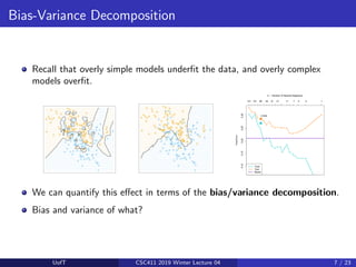
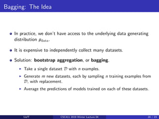
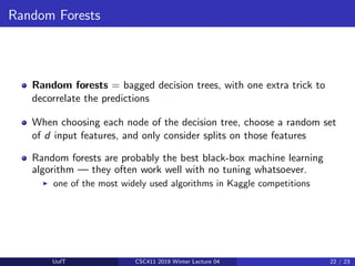
This lecture discusses ensemble methods in machine learning. It introduces bagging, which trains multiple models on random subsets of the training data and averages their predictions, in order to reduce variance and prevent overfitting. Bagging is effective because it decreases the correlation between predictions. Random forests apply bagging to decision trees while also introducing more randomness by selecting a random subset of features to consider at each node. The next lecture will cover boosting, which aims to reduce bias by training models sequentially to focus on examples previously misclassified.

1. CSC 411: Introduction to Machine Learning
Lecture 4: Ensemble I
Mengye Ren and Matthew MacKay
University of Toronto
UofT CSC411 2019 Winter Lecture 04 1 / 23

2. Overview
We’ve seen two particular learning algorithms: k-NN and decision trees
Next two lectures: combine multiple models into an ensemble which
performs better than the individual members
I Generic class of techniques that can be applied to almost any learning
algorithms...
I ... but are particularly well suited to decision trees
Today
I Understanding generalization using the bias/variance decomposition
I Reducing variance using bagging
Next lecture
I Making a weak classifier stronger (i.e. reducing bias) using boosting
UofT CSC411 2019 Winter Lecture 04 2 / 23

3. Ensemble methods: Overview
An ensemble of predictors is a set of predictors whose individual decisions
are combined in some way to predict new examples
I E.g., (possibly weighted) majority vote
For this to be nontrivial, the learned hypotheses must differ somehow, e.g.
I Different algorithm
I Different choice of hyperparameters
I Trained on different data
I Trained with different weighting of the training examples
Ensembles are usually easy to implement. The hard part is deciding what
kind of ensemble you want, based on your goals.
UofT CSC411 2019 Winter Lecture 04 3 / 23

4. Agenda
This lecture: bagging
I Train classifiers independently on random subsets of the training data.
Next lecture: boosting
I Train classifiers sequentially, each time focusing on training examples
that the previous ones got wrong.
Bagging and boosting serve very different purposes. To understand
this, we need to take a detour to understand the bias and variance of
a learning algorithm.
UofT CSC411 2019 Winter Lecture 04 4 / 23

5. Loss Functions
A loss function L(y, t) defines how bad it is if the algorithm predicts y, but
the target is actually t.
Example: 0-1 loss for classification
L0−1(y, t) =
(
0 if y = t
1 if y 6= t
I Averaging the 0-1 loss over the training set gives the training error
rate, and averaging over the test set gives the test error rate.
Example: squared error loss for regression
LSE(y, t) =
1
2
(y − t)2
I The average squared error loss is called mean squared error (MSE).
UofT CSC411 2019 Winter Lecture 04 5 / 23

6. Bias and Variance
UofT CSC411 2019 Winter Lecture 04 6 / 23

7. Bias-Variance Decomposition
Recall that overly simple models underfit the data, and overly complex
models overfit.
We can quantify this effect in terms of the bias/variance decomposition.
Bias and variance of what?
UofT CSC411 2019 Winter Lecture 04 7 / 23

8. Bias-Variance Decomposition: Basic Setup
Suppose the training set D consists of pairs (xi , ti ) sampled independent
and identically distributed (i.i.d.) from a single data generating
distribution pdata.
Pick a fixed query point x (denoted with a green x).
Consider an experiment where we sample lots of training sets independently
from pdata.
UofT CSC411 2019 Winter Lecture 04 8 / 23

9. Bias-Variance Decomposition: Basic Setup
Let’s run our learning algorithm on each training set, and compute its
prediction y at the query point x.
We can view y as a random variable, where the randomness comes from the
choice of training set.
The classification accuracy is determined by the distribution of y.
UofT CSC411 2019 Winter Lecture 04 9 / 23

10. Bias-Variance Decomposition: Basic Setup
Here is the analogous setup for regression:
Since y is a random variable, we can talk about its expectation, variance, etc.
UofT CSC411 2019 Winter Lecture 04 10 / 23

11. Bias-Variance Decomposition: Basic Setup
Recap of basic setup:
!"#$
{ &(()
, +(()
}
&, +
Training set
Test query
Data
S
a
m
p
l
e
S
a
m
p
l
e
ℎ
Learning
. Prediction
Hypothesis
&
/
Loss
+
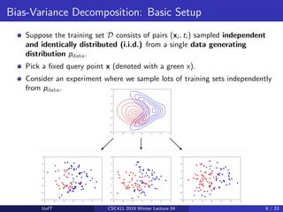
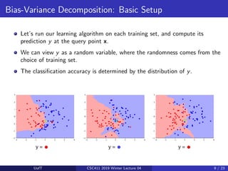
Notice: y is independent of t. (Why?)
This gives a distribution over the loss at x, with expectation E[L(y, t) | x].
For each query point x, the expected loss is different. We are interested in
minimizing the expectation of this with respect to x ∼ pdata.
UofT CSC411 2019 Winter Lecture 04 11 / 23

12. Bayes Optimality
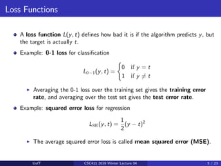
For now, focus on squared error loss, L(y, t) = 1
2 (y − t)2
.
A first step: suppose we knew the conditional distribution p(t | x). What
value y should we predict?
I Here, we are treating t as a random variable and choosing y.
Claim: y∗ = E[t | x] is the best possible prediction.
Proof:
E[(y − t)2
| x] = E[y2
− 2yt + t2
| x]
= y2
− 2yE[t | x] + E[t2
| x]
= y2
− 2yE[t | x] + E[t | x]2
+ Var[t | x]
= y2
− 2yy∗ + y2
∗ + Var[t | x]
= (y − y∗)2
+ Var[t | x]
UofT CSC411 2019 Winter Lecture 04 12 / 23

13. Bayes Optimality
E[(y − t)2
| x] = (y − y∗)2
+ Var[t | x]
The first term is nonnegative, and can be made 0 by setting y = y∗.
The second term corresponds to the inherent unpredictability, or noise, of
the targets, and is called the Bayes error.
I This is the best we can ever hope to do with any learning algorithm.
An algorithm that achieves it is Bayes optimal.
I Notice that this term doesn’t depend on y.
This process of choosing a single value y∗ based on p(t | x) is an example of
decision theory.
UofT CSC411 2019 Winter Lecture 04 13 / 23

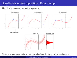
14. Bayes Optimality
Now return to treating y as a random variable (where the randomness
comes from the choice of dataset).
We can decompose out the expected loss (suppressing the conditioning on x
for clarity):
E[(y − t)2
] = E[(y − y∗)2
] + Var(t)
= E[y2
∗ − 2y∗y + y2
] + Var(t)
= y2
∗ − 2y∗E[y] + E[y2
] + Var(t)
= y2
∗ − 2y∗E[y] + E[y]2
+ Var(y) + Var(t)
= (y∗ − E[y])2
| {z }
bias
+ Var(y)
| {z }
variance
+ Var(t)
| {z }
Bayes error
UofT CSC411 2019 Winter Lecture 04 14 / 23

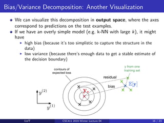
15. Bayes Optimality
E[(y − t)2
] = (y∗ − E[y])2
| {z }
bias
+ Var(y)
| {z }
variance
+ Var(t)
| {z }
Bayes error
We just split the expected loss into three terms:
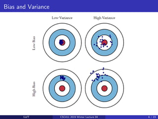
I bias: how wrong the expected prediction is (corresponds to
underfitting)
I variance: the amount of variability in the predictions (corresponds to
overfitting)
I Bayes error: the inherent unpredictability of the targets
Even though this analysis only applies to squared error, we often loosely use
“bias” and “variance” as synonyms for “underfitting” and “overfitting”.
UofT CSC411 2019 Winter Lecture 04 15 / 23

16. Bias/Variance Decomposition: Another Visualization
We can visualize this decomposition in output space, where the axes
correspond to predictions on the test examples.
If we have an overly simple model (e.g. k-NN with large k), it might
have
I high bias (because it’s too simplistic to capture the structure in the
data)
I low variance (because there’s enough data to get a stable estimate of
the decision boundary)
UofT CSC411 2019 Winter Lecture 04 16 / 23

17. Bias/Variance Decomposition: Another Visualization
If you have an overly complex model (e.g. k-NN with k = 1), it might
have
I low bias (since it learns all the relevant structure)
I high variance (it fits the quirks of the data you happened to sample)
UofT CSC411 2019 Winter Lecture 04 17 / 23

18. Bagging
Now, back to bagging!
UofT CSC411 2019 Winter Lecture 04 18 / 23

19. Bagging: Motivation
Suppose we could somehow sample m independent training sets from
pdata.
We could then compute the prediction yi based on each one, and take
the average y = 1
m
Pm
i=1 yi .
How does this affect the three terms of the expected loss?
I Bayes error: unchanged, since we have no control over it
I Bias: unchanged, since the averaged prediction has the same
expectation
E[y] = E
"
1
m
m
X
i=1
yi
#
= E[yi ]
I Variance: reduced, since we’re averaging over independent samples
Var[y] = Var
"
1
m
m
X
i=1
yi
#
=
1
m2
m
X
i=1
Var[yi ] =
1
m
Var[yi ].
UofT CSC411 2019 Winter Lecture 04 19 / 23

20. Bagging: The Idea
In practice, we don’t have access to the underlying data generating
distribution pdata.
It is expensive to independently collect many datasets.
Solution: bootstrap aggregation, or bagging.
I Take a single dataset D with n examples.
I Generate m new datasets, each by sampling n training examples from
D, with replacement.
I Average the predictions of models trained on each of these datasets.
UofT CSC411 2019 Winter Lecture 04 20 / 23

21. Bagging: The Idea
Problem: the datasets are not independent, so we don’t get the 1/m
variance reduction.
I Possible to show that if the sampled predictions have variance σ2
and
correlation ρ, then
Var
1
m
m
X
i=1
yi
!
=
1
m
(1 − ρ)σ2
+ ρσ2
.
Ironically, it can be advantageous to introduce additional variability
into your algorithm, as long as it reduces the correlation between
samples.
I Intuition: you want to invest in a diversified portfolio, not just one
stock.
I Can help to use average over multiple algorithms, or multiple
configurations of the same algorithm.
UofT CSC411 2019 Winter Lecture 04 21 / 23

22. Random Forests
Random forests = bagged decision trees, with one extra trick to
decorrelate the predictions
When choosing each node of the decision tree, choose a random set
of d input features, and only consider splits on those features
Random forests are probably the best black-box machine learning
algorithm — they often work well with no tuning whatsoever.
I one of the most widely used algorithms in Kaggle competitions
UofT CSC411 2019 Winter Lecture 04 22 / 23

23. Summary
Bagging reduces overfitting by averaging predictions.
Used in most competition winners
I Even if a single model is great, a small ensemble usually helps.
Limitations:
I Does not reduce bias.
I There is still correlation between classifiers.
Random forest solution: Add more randomness.
UofT CSC411 2019 Winter Lecture 04 23 / 23