Download to read offline
![Machine Learning and Applications: An International Journal (MLAIJ) Vol.11, No. 4, December 2024
DOI:10.5121/mlaij.2024.11401 1
ϵ
EMPIRICAL ANALYSIS OF THE BIAS-VARIANCE
TRADEOFF ACROSS MACHINE LEARNING MODELS
Hardev Ranglani
EXL Service Inc.
ABSTRACT
Understanding the bias-variance tradeoff is pivotal for selecting optimal machine learning models. This
paper empirically examines bias, variance, and mean squared error (MSE) across regression and
classification datasets, using models ranging from decision tree to ensemble methods like random forest
and gradient boost. Results show that ensemble methods such as Random Forest, Gradient Boosting and
XGBoost consistently achieve the best tradeoff between bias and variance, resulting in the lowest overall
error while simpler models such as Decision Tree and k-NN can have either high bias or high variance.
This analysis bridges the gap between the theoretical bias-variance concepts and practical model
selection, and offers in- sights into algorithm performance across diverse datasets. Insights from this work
can guide practitioners in model selection, balancing predictive performance and interpretability
KEYWORDS
Bias, Variance, Mean SquaredError, Model Complexity, Bias-Variance Tradeoff
1. INTRODUCTION
For machine learning models, achieving optimal model performance is often a delicate balance
between Bias and Variance, a concept known as the Bias-Variance tradeoff. This tradeoff is
important because it determines a model’s ability to generalize to unseen data, which is the
most important way to measure model performance.
The overall error of a Machine Learning model is generally measured in terms of the Mean
Squared Error. It tells us the expected value of the sqaure of the difference between the predicted
value and the true value. The MSE for a model’s predictions can be written as :
MSE = E[(yˆ − y)2
]
where:
• y is the true value for an observation
• yˆ is the predicted value for an observation
• The expectation E[.] is taken over different training samples This can be further
decomposed as :
MSE = Bias2
+ Variance + IrreducibleError
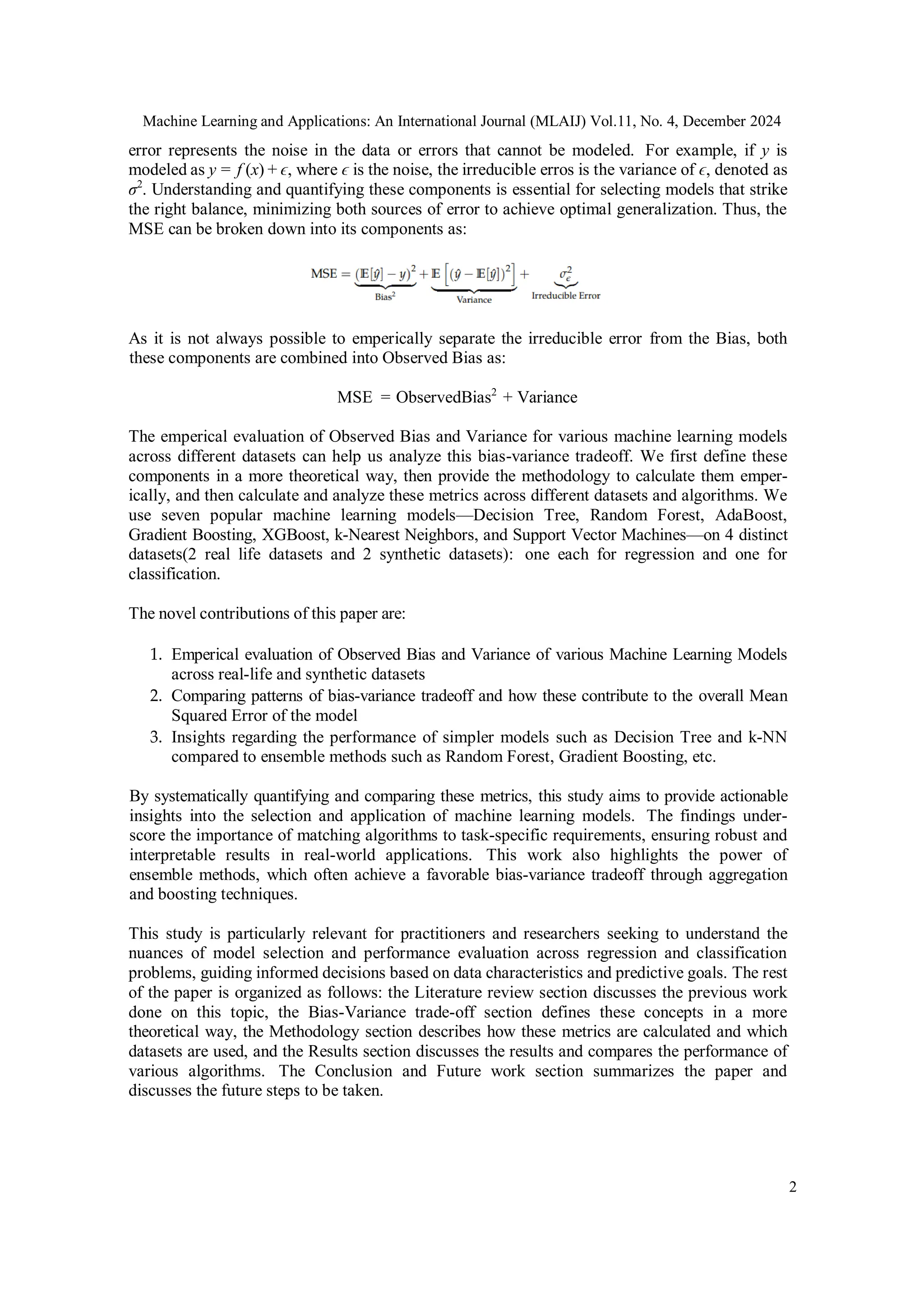
Bias represents the error introduced by oversimplifying the model, leading to systematic inac-
curacies in capturing the underlying data patterns. Variance measures a model’s sensitivity to
fluctuations in the training data, reflecting its tendency to overfit. These two sources of error are
inherently in conflict: reducing bias often increases variance and vice versa. The Irreducible](https://image.slidesharecdn.com/11424mlaij01-250102105733-f5a74fbb/75/Empirical-Analysis-of-the-Bias-Variance-Tradeoff-Across-Machine-Learning-Models-1-2048.jpg)
![Machine Learning and Applications: An International Journal (MLAIJ) Vol.11, No. 4, December 2024
4
framework to understand how different models behave in diverse scenarios. This comparison
offers actionable insights for practitioners, bridging theoretical concepts with practical applica-
tions, and establishing guidelines for model selection based on dataset characteristics such as
complexity, noise, and feature interactions.
3. BIAS-VARIANCE TRADEOFF: UNDERSTANDING AND QUANTIFYING
ERROR
The bias-variance tradeoff is a critical concept in machine learning that affects model selection
and performance optimization. It describes the interaction between two sources of error: bias,
which arises from over-simplifications in the model, and variance, which reflects the model’s
sensitivity to variations in the training data. Striking the right balance between bias and variance is
essential to minimize the total prediction error, enabling a model to generalize effectively to
unseen data. Figure 1 shows how the Mean Squared Error is influenced by the balance between
Bias2
and Variance as the model complexity increases as a U-curve. The curve for MSE is an
addition of Bias2
and Variance, with its minimum point indicating the optimal model complexity
that balances bias and variance for the best generalization.
Figure 1: Effect of model complexity on Bias, Variance and Total Error.
The total error of a model, often measured using the Mean Squared Error (MSE), can be
decomposed into three components: bias, variance, and irreducible error. Mathematically, this is
expressed as follows:
MSE = Bias2
+ Variance + IrreducibleError
Each of these components contributes uniquely to the performance of the model. Bias measures
the systematic error introduced when the model oversimplifies the true underlying function f
(x). It can be quantified as:
Bias2
= E[fˆ(x)] − f (x)
2
where E[ fˆ(x)] is the expected prediction of the model, averaged over all possible training
datasets. Models with high bias, such as linear regression applied to nonlinear data, fail to
capture the complexity of the underlying relationships, leading to underfitting.
Variance, on the other hand, measures the variability of the model predictions when trained on
different samples of the data. It is calculated as follows:](https://image.slidesharecdn.com/11424mlaij01-250102105733-f5a74fbb/75/Empirical-Analysis-of-the-Bias-Variance-Tradeoff-Across-Machine-Learning-Models-4-2048.jpg)
![Machine Learning and Applications: An International Journal (MLAIJ) Vol.11, No. 4, December 2024
5
N
N
Variance = E fˆ(x) − E[fˆ(x)]
2
High-variance models, such as unregularized decision trees, tend to overfit, as they capture
noise in the training data in addition to the true patterns. This makes them highly sensitive to
fluctuations in the data.
The irreducible error accounts for the inherent noise in the data, represented as ϵ in the equation y =
f (x) + ϵ, where ϵ ∼ N (0, σ2
). This component reflects random factors or measurement errors
that cannot be modeled or predicted, regardless of the complexity of the model.
In real-world datasets, the true function f (x) is unknown, making it difficult to directly measure
bias and variance. Instead, the squared observed bias often includes both the true bias and the
irreducible error. As a result, the estimated bias squared is given by:
ObservedBias2
= TrueBias2
+ σ2
.
This inherent challenge with the irreducible error means that, while variance can be accurately
computed, bias estimates inherently combine systematic error or true bias and noise.
To empirically measure bias, variance, and MSE for a machine learning model, a practical
approach involves bootstrap sampling. By generating multiple training data sets through
resampling and training the model on each, we can compute key metrics for a given test set. For
each test data point xi, the average prediction is :
ˆ 1 ˆ
E[f (xi)] = ∑ fj(xi)
j=1
where fˆj (xi) is the prediction from the j-th bootstrap sample, n is the total number of observations in
the dataset and N is the total number of bootstrap samples. Using these predictions, bias
squared can be estimated as:
and the variance is calculated as:
Finally, the total MSE for the test set is:
In practical applications, these computations provide valuable insights into the behavior of
different machine learning models. High-bias models tend to underfit, resulting in poor perfor-
mance on complex datasets, while high-variance models overfit and fail to generalize. Ensemble
methods, such as Random Forests and Gradient Boosting, achieve a favorable trade-off by re-
ducing variance without significantly increasing bias, making them well-suited for a wide range of](https://image.slidesharecdn.com/11424mlaij01-250102105733-f5a74fbb/75/Empirical-Analysis-of-the-Bias-Variance-Tradeoff-Across-Machine-Learning-Models-5-2048.jpg)
![Machine Learning and Applications: An International Journal (MLAIJ) Vol.11, No. 4, December 2024
7
4.3. Experimental Setup
Seven machine learning algorithms were applied to all four datasets: Decision Tree, Random
Forest, AdaBoost, Gradient Boosting, XGBoost, k-Nearest Neighbors (k-NN) and Support Vector
Machines (SVM). These models were chosen for their diverse mechanisms, from simple tree-
based learners to ensemble methods and distance-based classifiers, providing a spectrum of
complexity and interpretability.
To analyze the bias-variance tradeoff, bootstrap sampling was employed:
4.3.1. The data was split into a random but stratified 70-30 train test split and from the training
data for each dataset, 100 bootstrap samples of size 70% of the size of the original dataset
were generated by sampling with replacement.
4.3.2. Each model was trained on these bootstrap samples and predictions were made on the
test set.
4.3.3. For each test data point, the average prediction and its variability were calculated across
bootstrap iterations.
Bias and variance were estimated using the following equations
where fˆj (xi) represents the prediction for the test point xi from the j-th bootstrap model, n is
the number of observations in the sample, N is the number of bootstrap samples and E[ fˆ(xi)] is
the mean prediction across all bootstrap samples.
The Mean Squared Error (MSE) is then decomposed into its components.
MSE = TrueBias2
+ Variance + σ2
, as the irreducible error cannot be directly measured, it is combined with the True Bias to form
observed bias as:
MSE = ObservedBias2
+ Variance
These metrics are calculated and compared across all ML models for a given dataset](https://image.slidesharecdn.com/11424mlaij01-250102105733-f5a74fbb/75/Empirical-Analysis-of-the-Bias-Variance-Tradeoff-Across-Machine-Learning-Models-7-2048.jpg)
![Machine Learning and Applications: An International Journal (MLAIJ) Vol.11, No. 4, December 2024
12
also remains an open area of work. This work lays the foundation for selecting robust models
and balancing predictive accuracy with generalizability in diverse machine learning tasks.
REFERENCES
[1] Geman, S., Bienenstock, E., & Doursat, R. (1992). Neural networks and the bias/variance dilemma.
Neural Computation, 4(1), 1-58.
[2] Harrell, F. E. (2001). Regression Modeling Strategies: With Applications to Linear Models, Logistic
Regression, and Survival Analysis. Springer.
[3] Breiman, L. (2001). Random forests. Machine Learning, 45(1), 5-32.
[4] Friedman, J. H. (2001). Greedy function approximation: A gradient boosting machine. Annals of
Statistics, 29(5), 1189-1232.
[5] Vapnik, V. N. (1995). The Nature of Statistical Learning Theory. Springer.
[6] Cover, T., & Hart, P. (1967). Nearest neighbor pattern classification. IEEE Transactions on
Information Theory, 13(1), 21-27.
[7] Willmott, C. J., & Matsuura, K. (2005). Advantages of the mean absolute error over the root mean
squared error. Climate Research, 30(1), 79-82.
[8] Hyndman, R. J., & Koehler, A. B. (2006). Another look at measures of forecast accuracy.
International Journal of Forecasting, 22(4), 679-688.
[9] Murphy, K. P. (2012). Machine Learning: A Probabilistic Perspective. MIT Press.
[10] Berrar, D. (2019). Cross-Entropy Loss Function. In Encyclopedia of Bioinformatics and
Computational Biology: ABC of Bioinformatics (pp. 546-550). Elsevier.
[11] Domingos, P. (2000). A unified bias-variance decomposition for zero-one and squared loss. In
Proceedings of the Seventeenth International Conference on Machine Learning (pp. 231-238).
Morgan Kaufmann.
[12] Dietterich, T. G. (2000). Ensemble methods in machine learning. In Proceedings of the First
International Workshop on Multiple Classifier Systems (pp. 1-15). Springer.
[13] DanaFerguson, Meg Risdal, NoTrick, Sara R, Sillah, Tim Emmerling, and Will Cukierski. Allstate
Claims Severity. https://kaggle.com/competitions/allstate-claims-severity, 2016. Kaggle.
[14] Moro, S., Rita, P., & Cortez, P. (2014). Bank Marketing [Dataset]. UCI Machine Learning
Repository. https://doi.org/10.24432/C5K306.
[15] LeCun, Y., Bottou, L., Bengio, Y., & Haffner, P. (1998). Gradient-based learning applied to
document recognition. Proceedings of the IEEE, 86(11), 2278-2324.](https://image.slidesharecdn.com/11424mlaij01-250102105733-f5a74fbb/75/Empirical-Analysis-of-the-Bias-Variance-Tradeoff-Across-Machine-Learning-Models-12-2048.jpg)

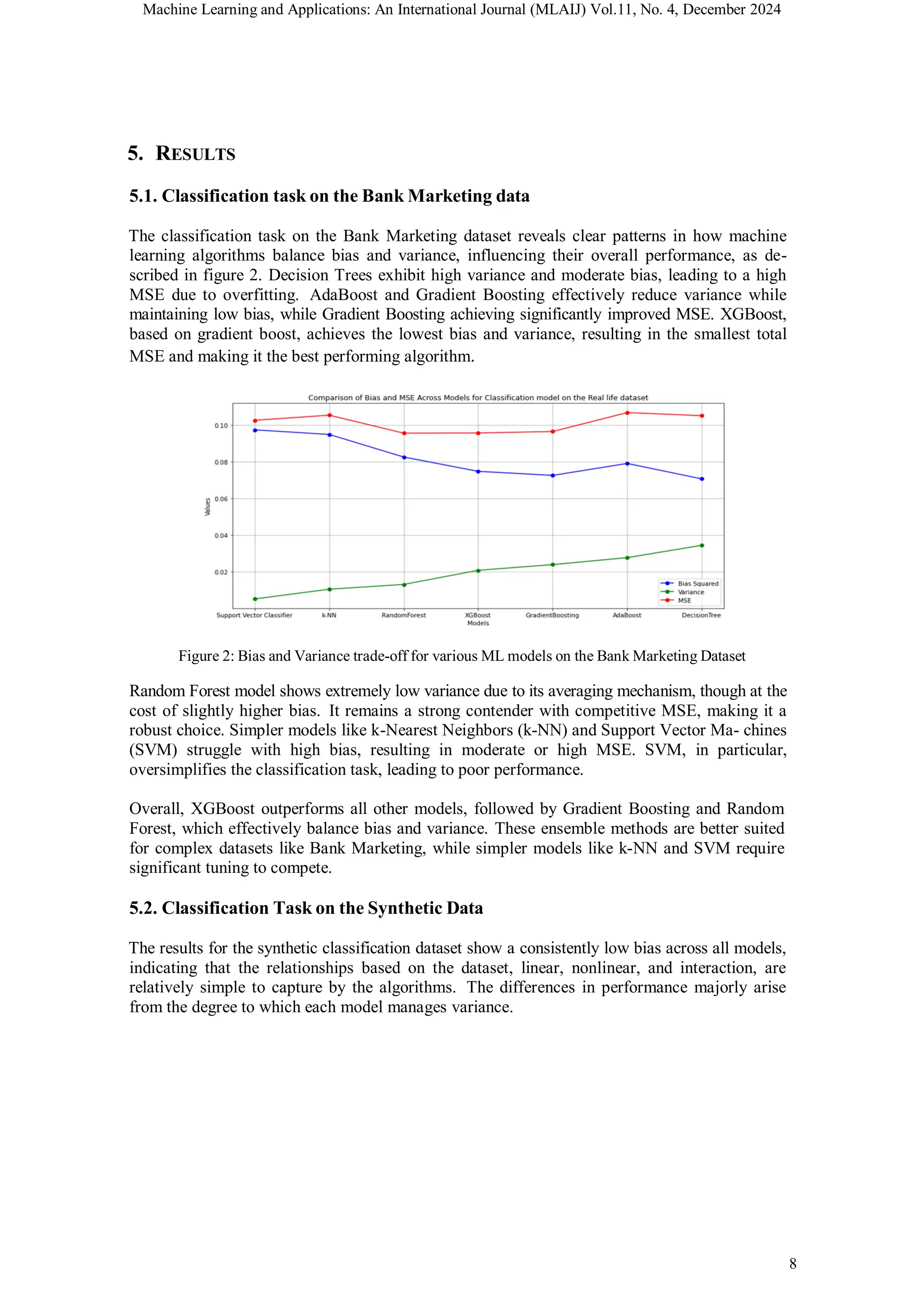
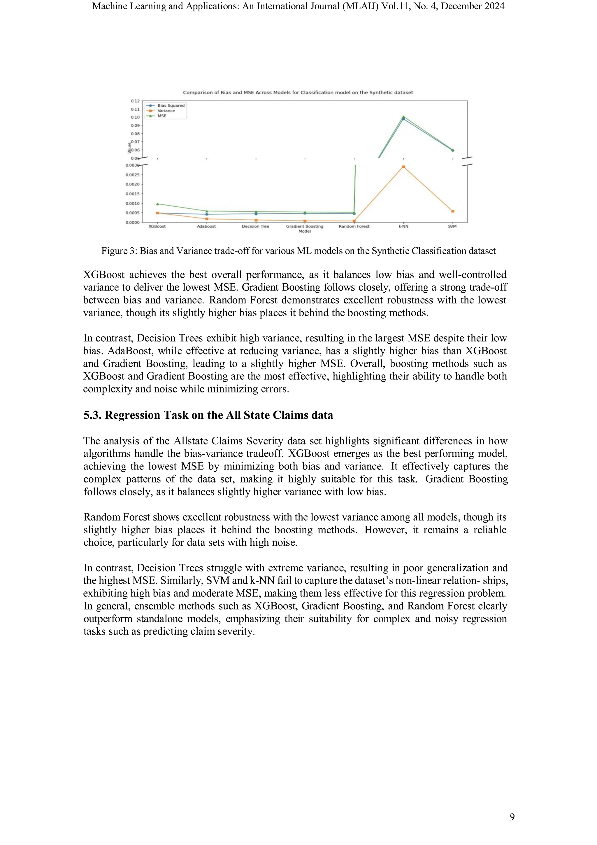
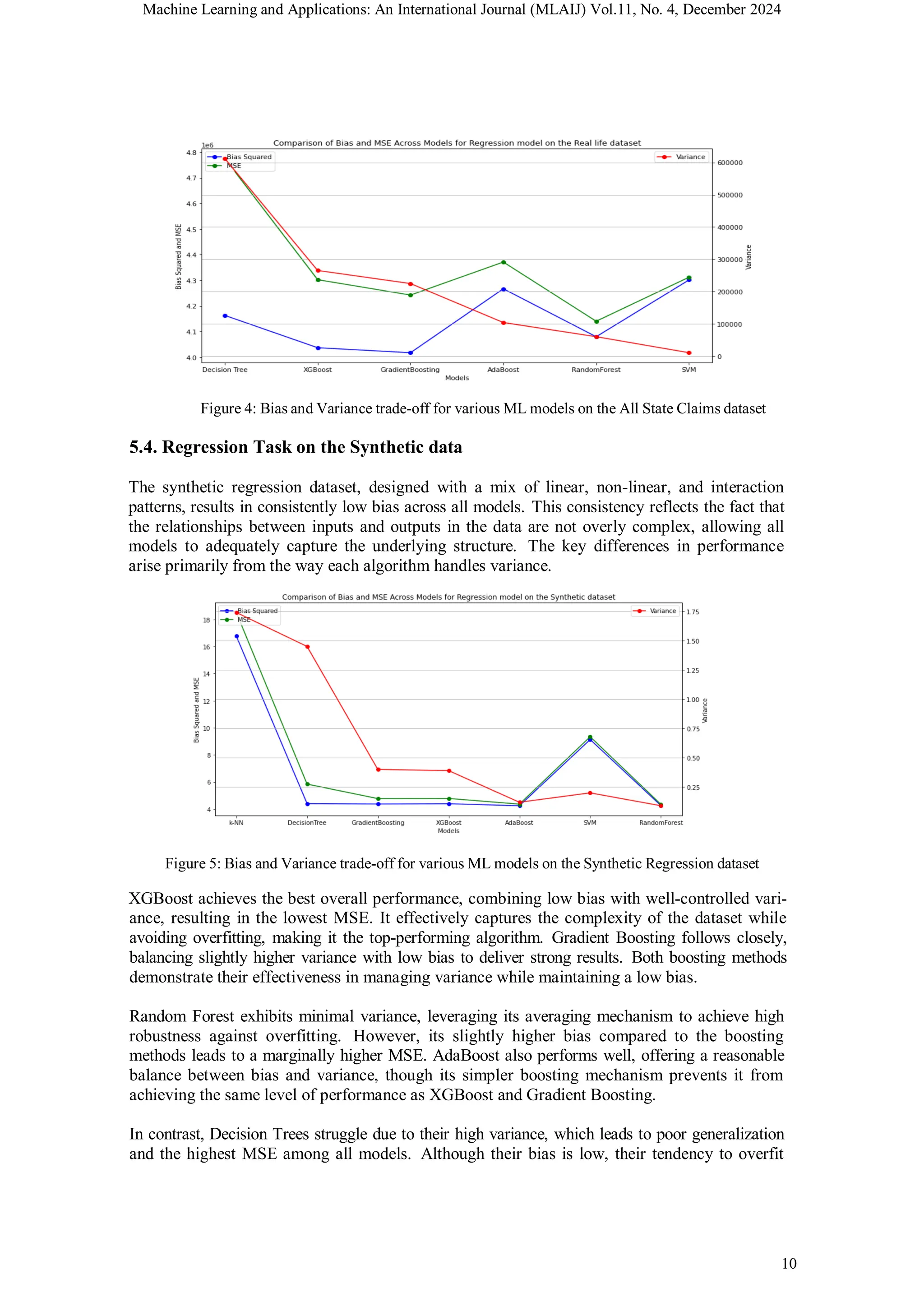
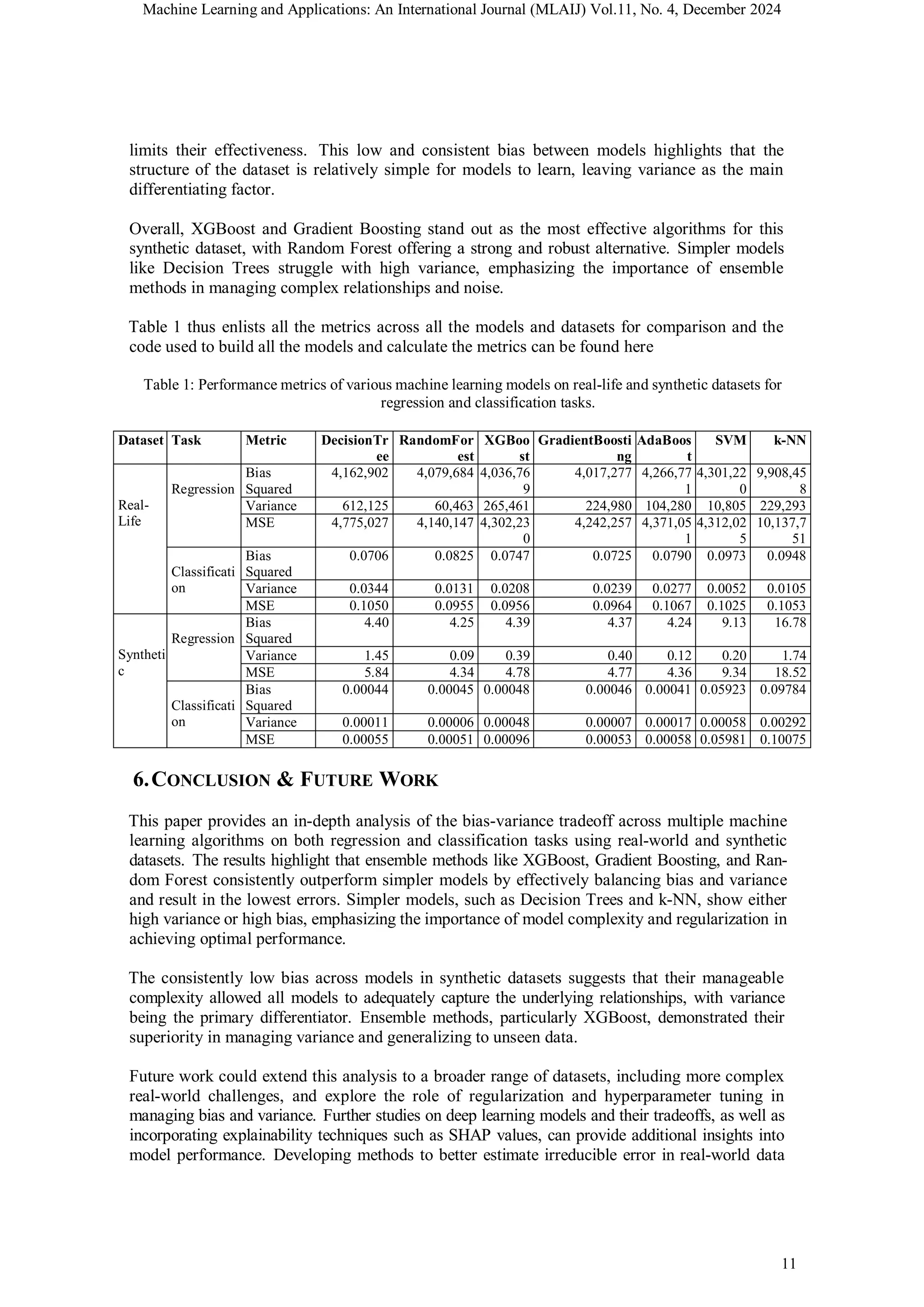
The document provides an empirical analysis of the bias-variance tradeoff in various machine learning models to guide model selection. It reviews the performance of seven models including decision trees and ensemble methods like random forest and gradient boosting across multiple datasets, highlighting that ensemble methods yield the best balance between bias and variance. This study aims to bridge theoretical concepts with practical applications, offering insights for practitioners on optimizing predictive performance.